
LungINFseg: Segmenting COVID-19 Infected Regions in Lung CT Images Based on a Receptive-Field-Aware Deep Learning Framework


Abstract
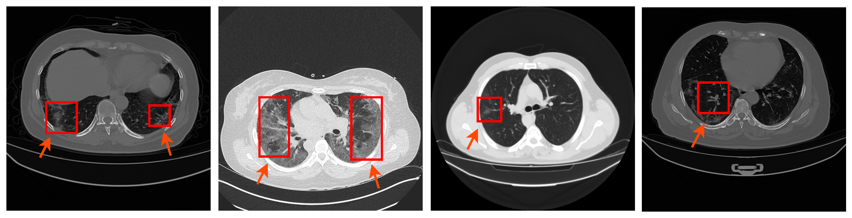
1. Introduction
- We propose a fully automated and efficient deep learning based method to segment the COVID-19 infection in lung CT images.
- We propose the RFA module that can enlarge the receptive field of the segmentation models and increase the learning ability of the model without information loss.
- Extensive experiments were performed to provide ablation studies that add a thorough analysis of the proposed LungINFSeg (e.g., the effect of resolution size and variation of the loss function). To reproduce the results, the source code of the proposed model is publicly available at https://github.com/vivek231/LungINFseg.
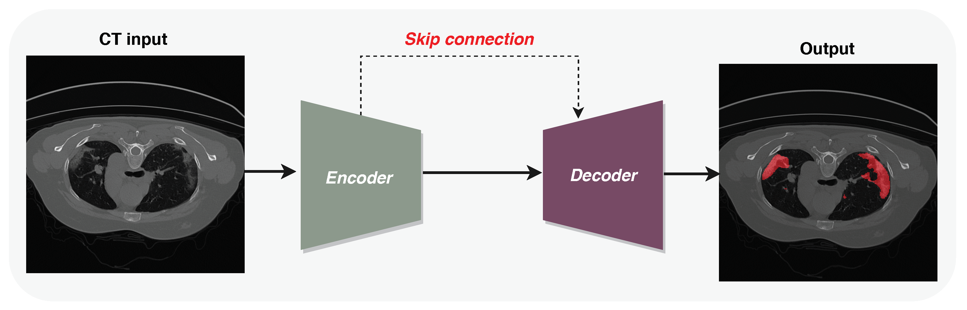
2. Methodology
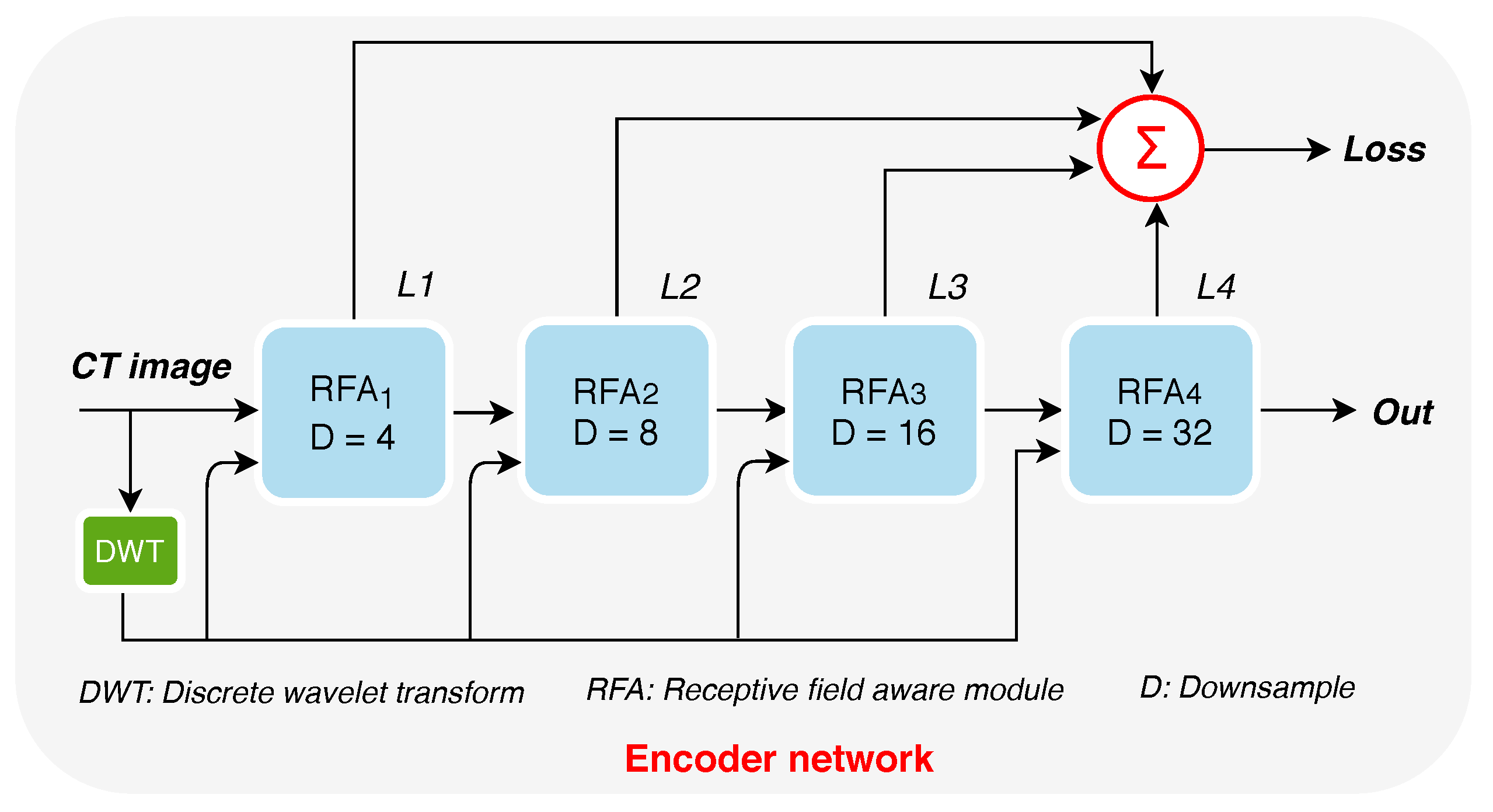
2.1. Encoder
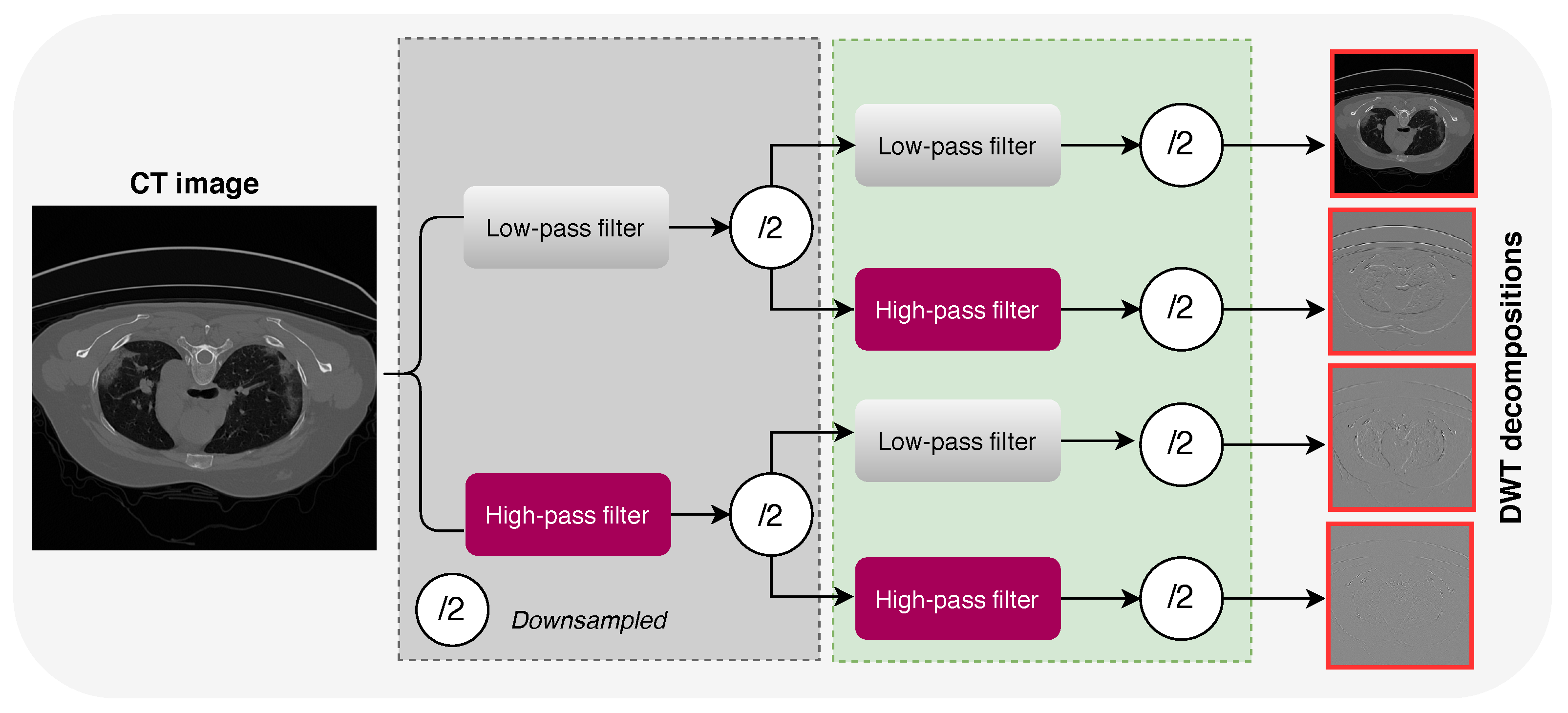
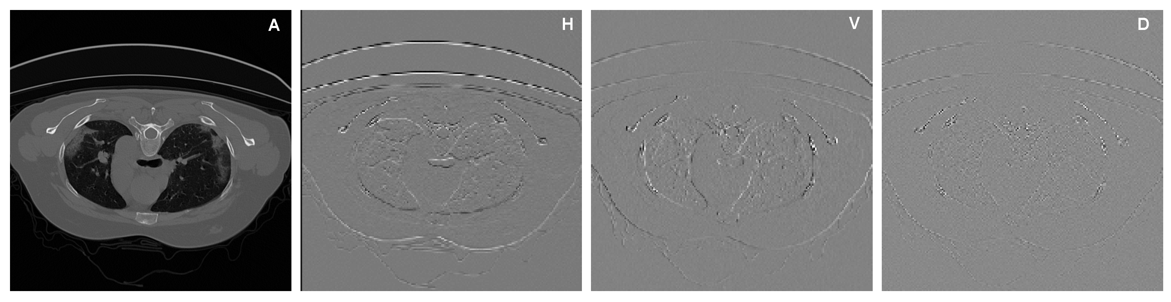
2.1.1. Increasing the Receptive Fields Using Discrete Wavelet Transform (DWT)
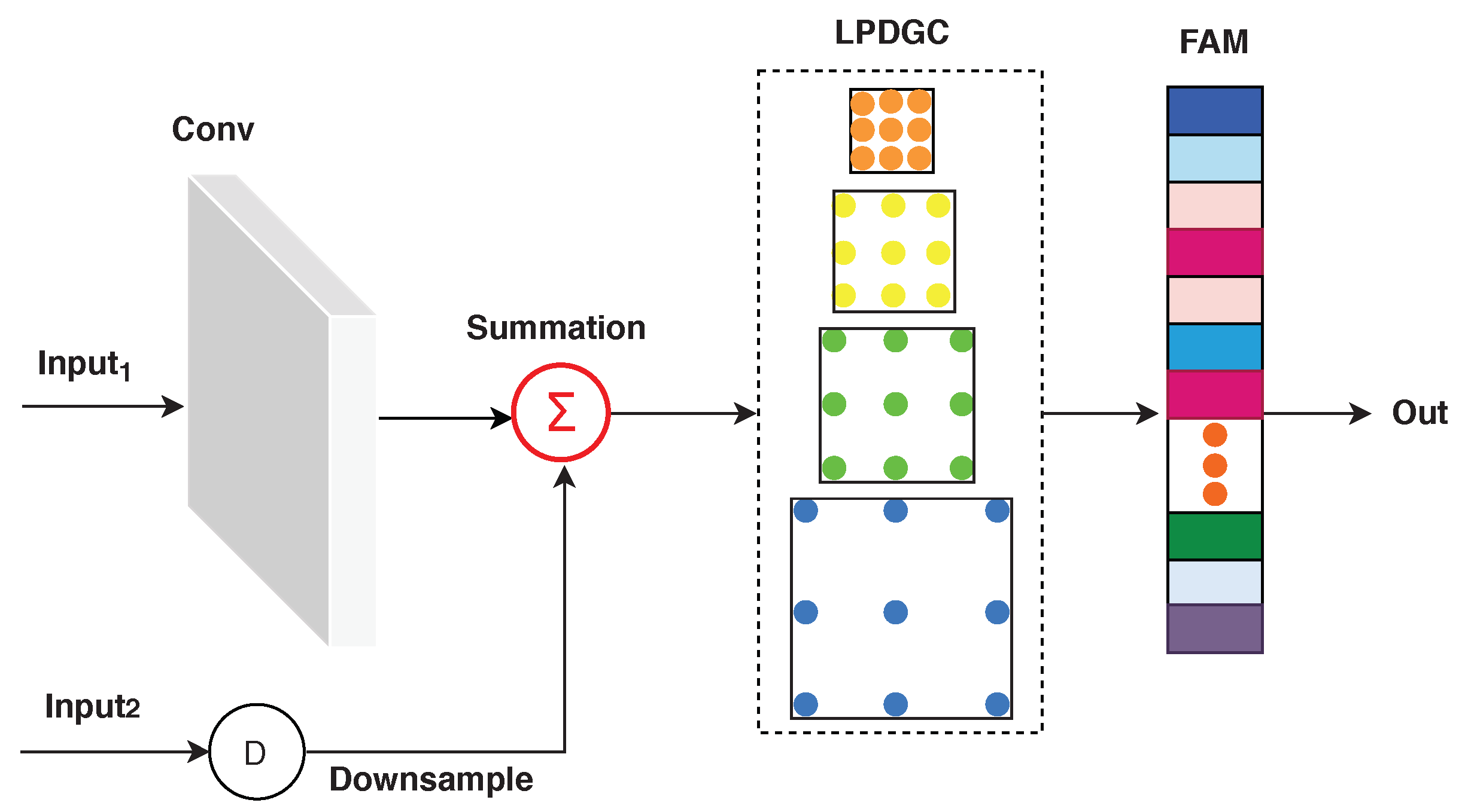
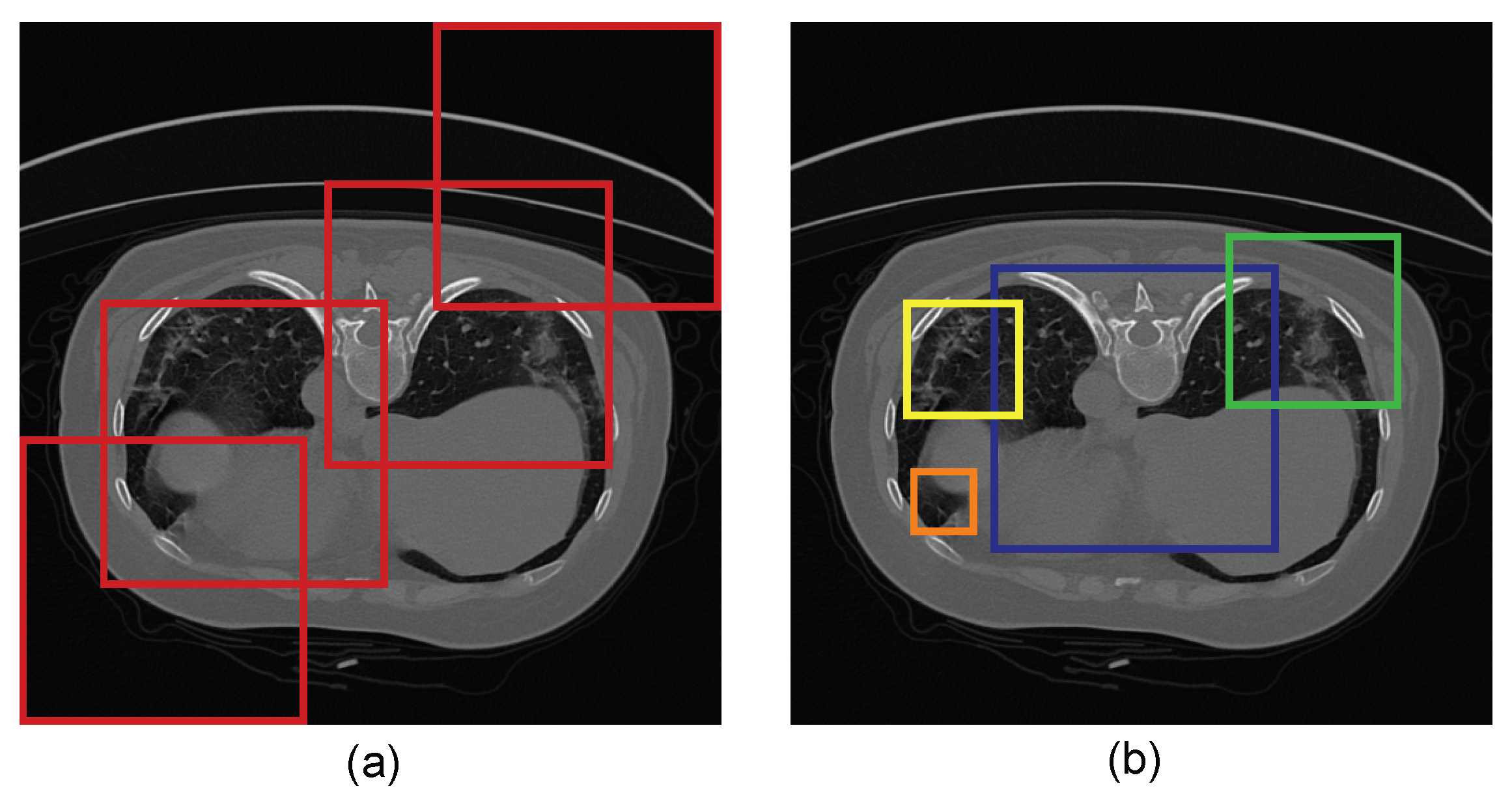
2.1.2. Receptive-Field-Aware (RFA) Module
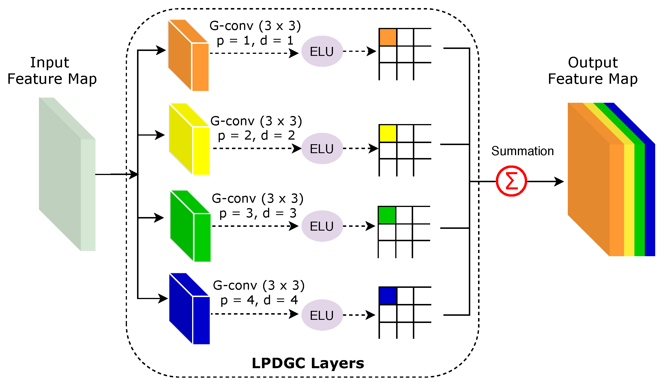
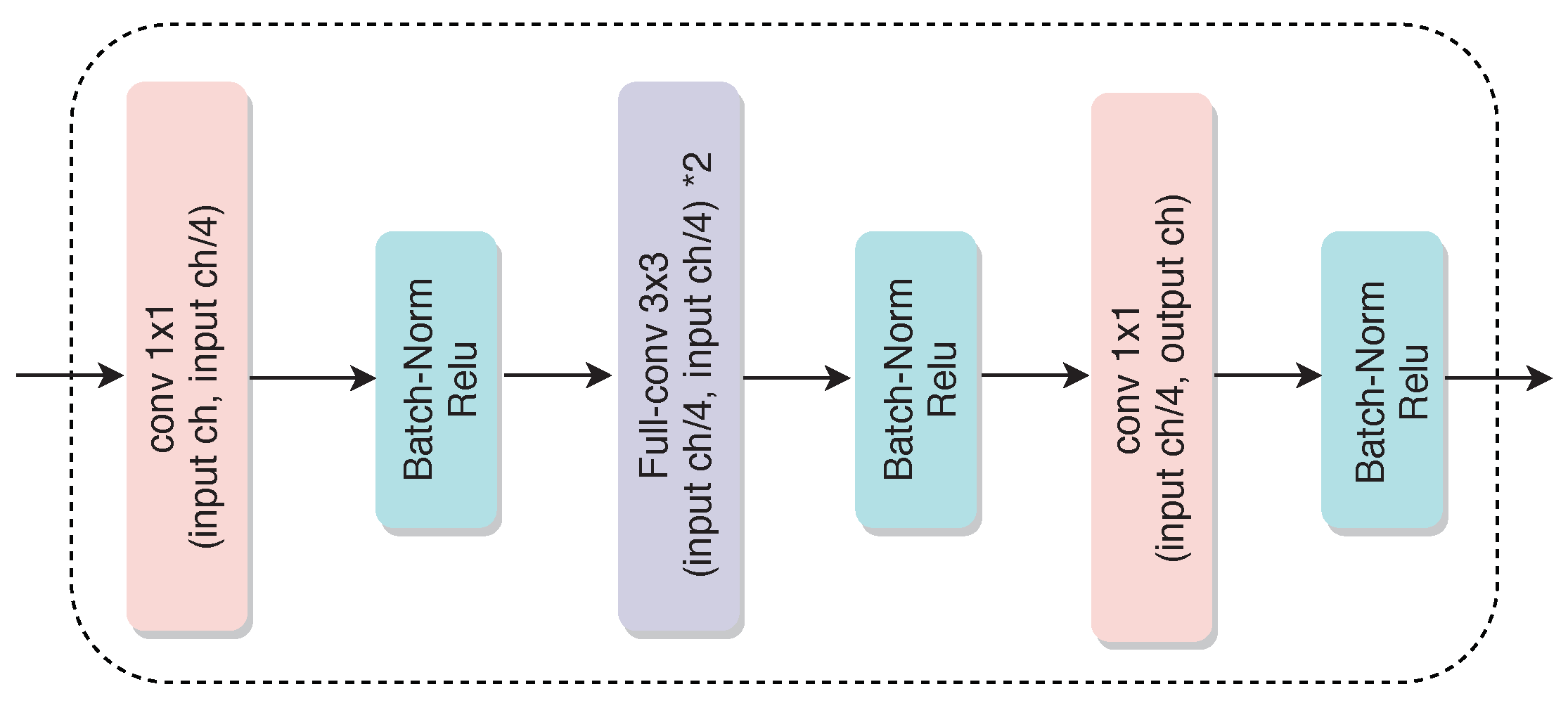
Learnable Parallel Dilated Group Convolutional (LPDGC) Block
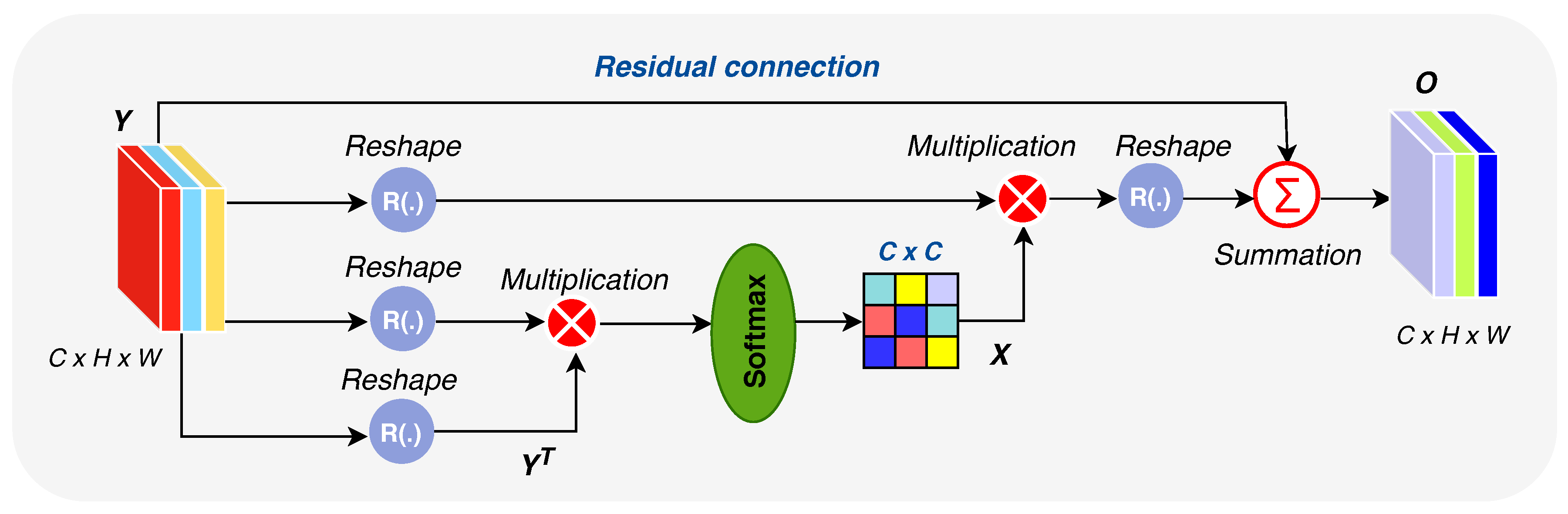
Feature Attention Module (FAM)
2.2. Decoder Network
2.3. Architecture of LungINFseg
2.4. Loss Functions
2.5. Evaluation Metrics
3. Experimental Results and Discussion
3.1. Experimental Details
3.1.1. COVID-19 Lung CT Dataset
3.1.2. Data Augmentation and Parameter Setting
3.2. Ablation Study
3.3. Analysis of the Performance of the Proposed Model
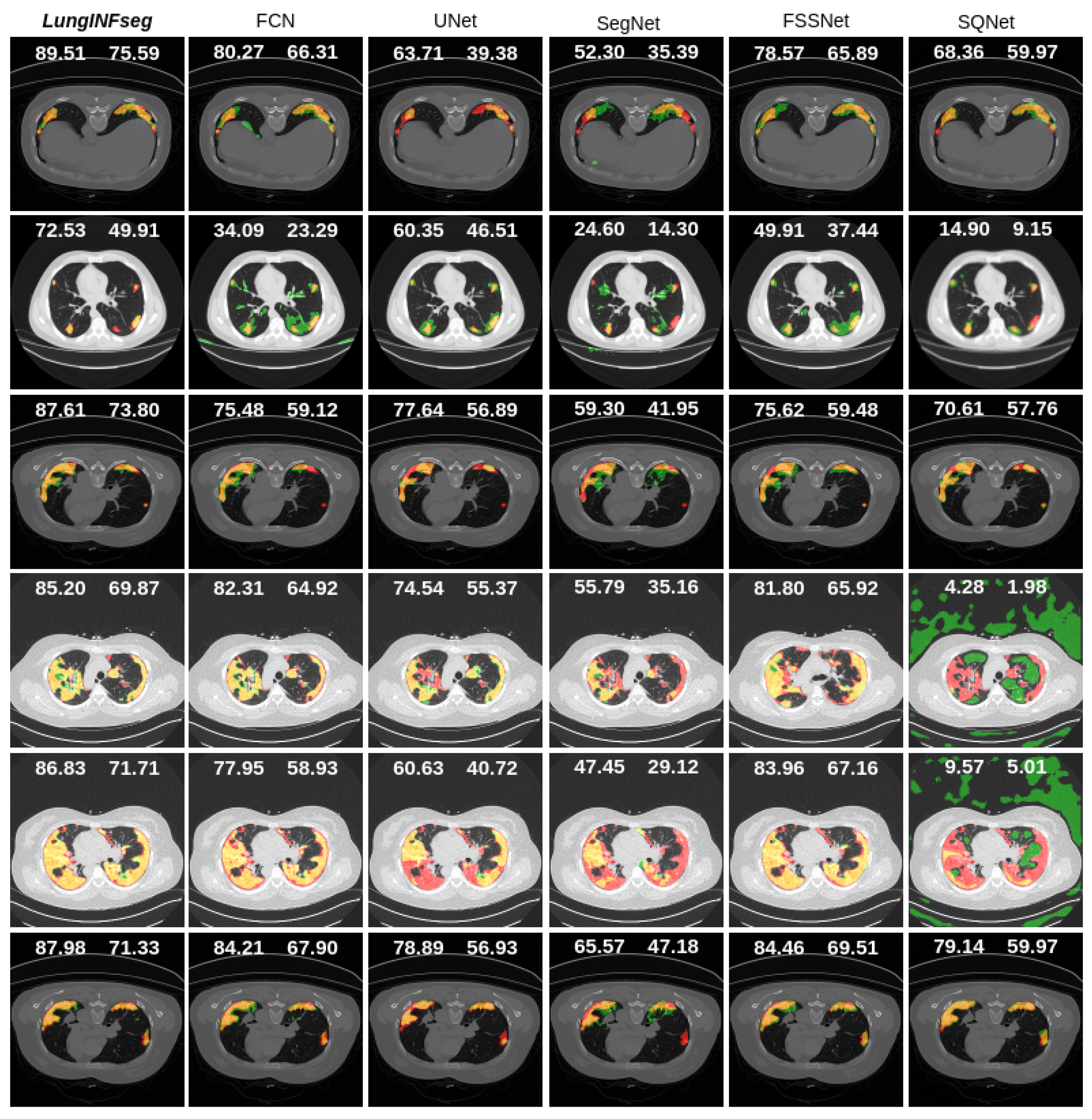
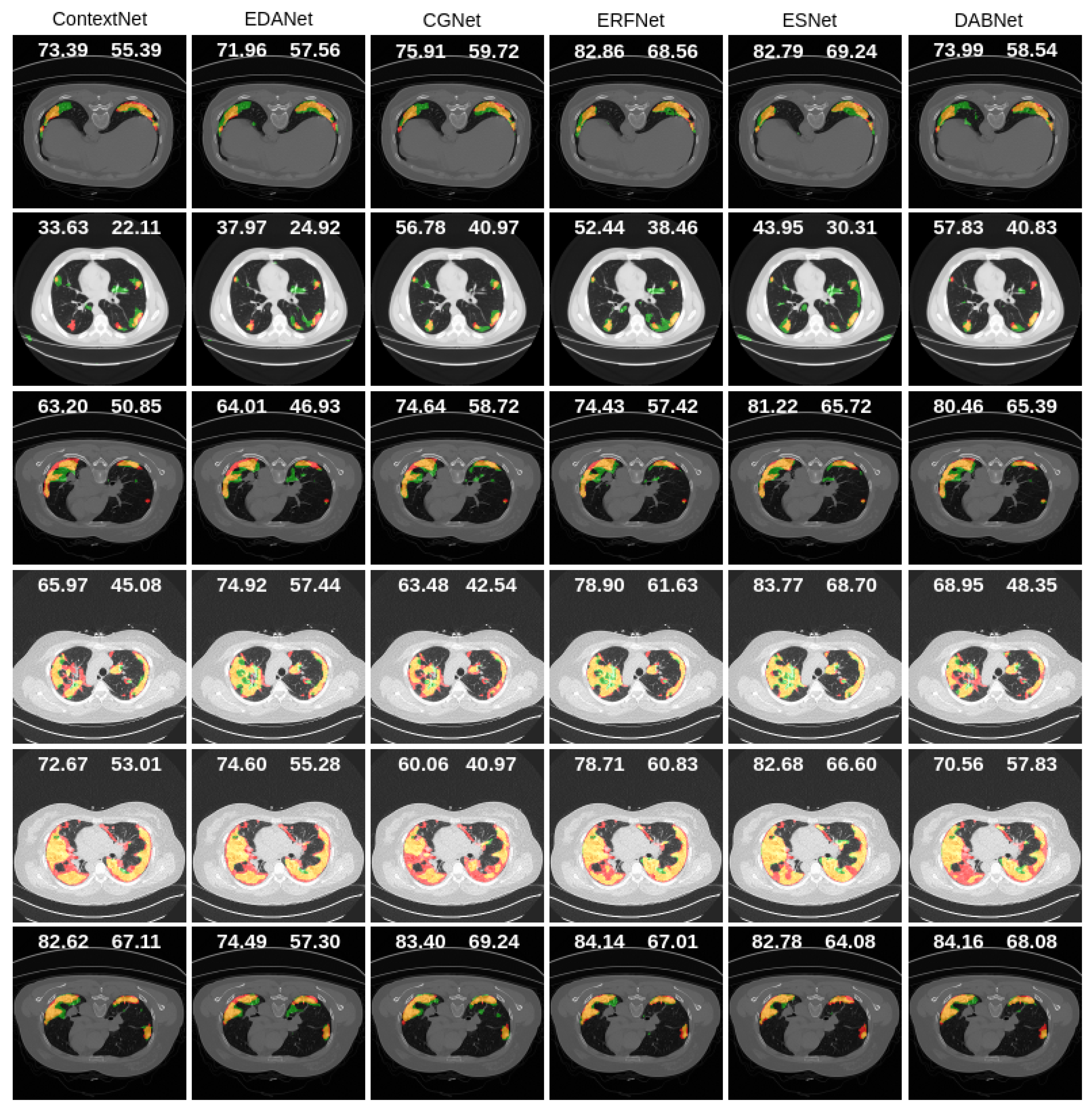
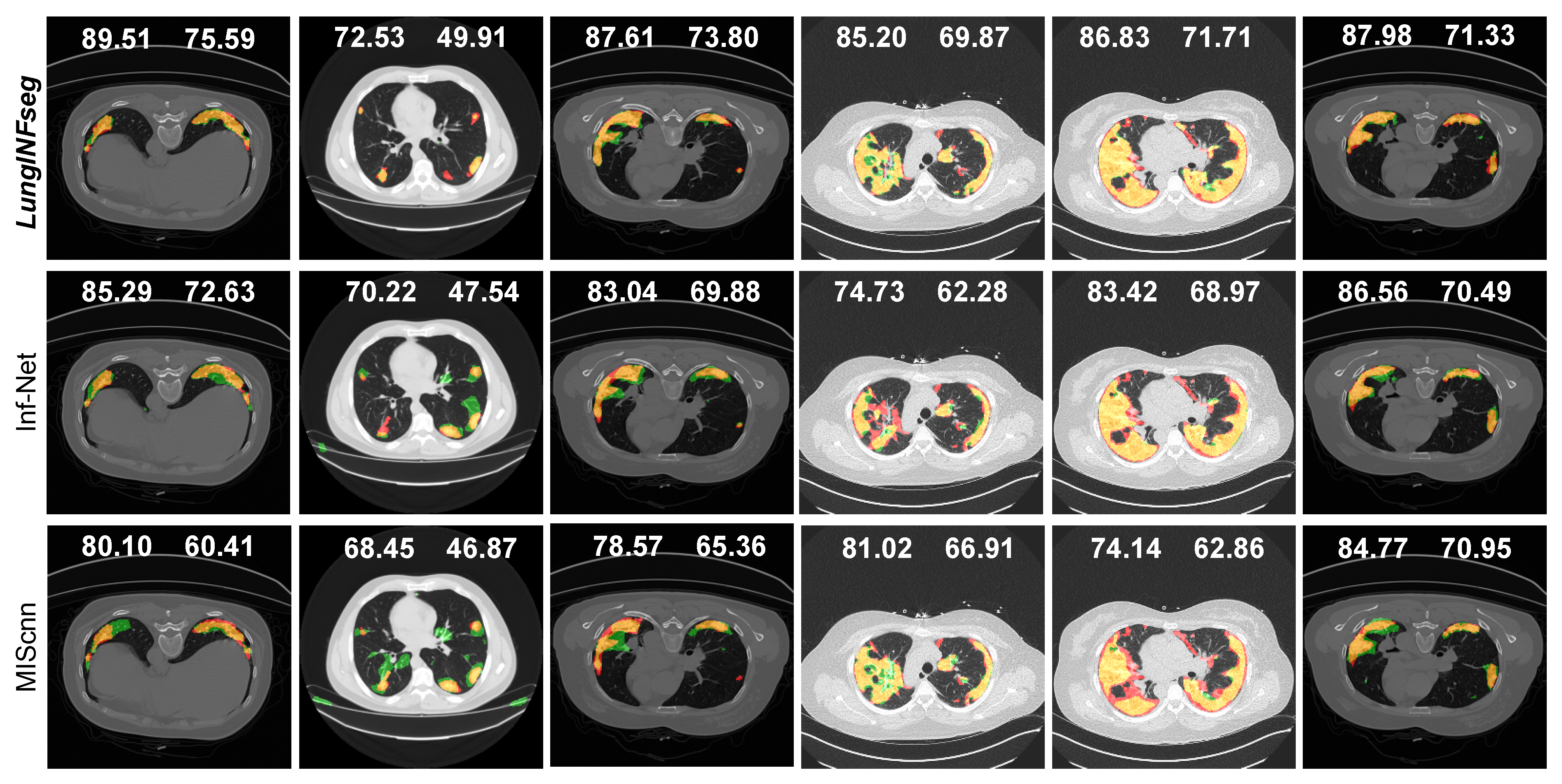
3.4. Comparisons with the State-of-the-Art
4. Conclusions
Author Contributions
Funding
Institutional Review Board Statement
Informed Consent Statement
Data Availability Statement
Acknowledgments
Conflicts of Interest
References
- World Health Organization. WHO Coronavirus Disease (COVID-19) Dashboard; World Health Organization: Geneva, Switzerland, 2020; Volume 5, Available online: Https://covid19.Who.Int (accessed on 25 June 2020).
- Dai, W.C.; Zhang, H.W.; Yu, J.; Xu, H.J.; Chen, H.; Luo, S.P.; Zhang, H.; Liang, L.H.; Wu, X.L.; Lei, Y.; et al. CT imaging and differential diagnosis of COVID-19. Can. Assoc. Radiol. J. 2020, 71, 195–200. [Google Scholar] [CrossRef] [PubMed]
- Ai, T.; Yang, Z.; Hou, H.; Zhan, C.; Chen, C.; Lv, W.; Tao, Q.; Sun, Z.; Xia, L. Correlation of chest CT and RT-PCR testing in coronavirus disease 2019 (COVID-19) in China: A report of 1014 cases. Radiology 2020, 296, 200642. [Google Scholar] [CrossRef] [PubMed]
- Salehi, S.; Abedi, A.; Balakrishnan, S.; Gholamrezanezhad, A. Coronavirus disease 2019 (COVID-19): A systematic review of imaging findings in 919 patients. Am. J. Roentgenol. 2020, 215, 1–7. [Google Scholar] [CrossRef] [PubMed]
- Casiraghi, E.; Malchiodi, D.; Trucco, G.; Frasca, M.; Cappelletti, L.; Fontana, T.; Esposito, A.A.; Avola, E.; Jachetti, A.; Reese, J.; et al. Explainable Machine Learning for Early Assessment of COVID-19 Risk Prediction in Emergency Departments. IEEE Access 2020, 8, 196299–196325. [Google Scholar] [CrossRef]
- Maguolo, G.; Nanni, L. A critic evaluation of methods for covid-19 automatic detection from x-ray images. arXiv 2020, arXiv:2004.12823. [Google Scholar]
- Giannitto, C.; Sposta, F.M.; Repici, A.; Vatteroni, G.; Casiraghi, E.; Casari, E.; Ferraroli, G.M.; Fugazza, A.; Sandri, M.T.; Chiti, A.; et al. Chest CT in patients with a moderate or high pretest probability of COVID-19 and negative swab. Radiol. Medica 2020, 125, 1260–1270. [Google Scholar] [CrossRef]
- Chen, X.; Yao, L.; Zhang, Y. Residual Attention U-Net for Automated Multi-Class Segmentation of COVID-19 Chest CT Images. arXiv 2020, arXiv:2004.05645. [Google Scholar]
- Yan, Q.; Wang, B.; Gong, D.; Luo, C.; Zhao, W.; Shen, J.; Shi, Q.; Jin, S.; Zhang, L.; You, Z. COVID-19 Chest CT Image Segmentation–A Deep Convolutional Neural Network Solution. arXiv 2020, arXiv:2004.10987. [Google Scholar]
- Voulodimos, A.; Protopapadakis, E.; Katsamenis, I.; Doulamis, A.; Doulamis, N. Deep learning models for COVID-19 infected area segmentation in CT images. medRxiv 2020. [Google Scholar] [CrossRef]
- Wang, G.; Liu, X.; Li, C.; Xu, Z.; Ruan, J.; Zhu, H.; Meng, T.; Li, K.; Huang, N.; Zhang, S. A Noise-robust Framework for Automatic Segmentation of COVID-19 Pneumonia Lesions from CT Images. IEEE Trans. Med. Imaging 2020, 39, 2653–2663. [Google Scholar] [CrossRef]
- Fan, D.P.; Zhou, T.; Ji, G.P.; Zhou, Y.; Chen, G.; Fu, H.; Shen, J.; Shao, L. Inf-Net: Automatic COVID-19 Lung Infection Segmentation from CT Scans. arXiv 2020, arXiv:2004.14133. [Google Scholar]
- Müller, D.; Rey, I.S.; Kramer, F. Automated Chest CT Image Segmentation of COVID-19 Lung Infection based on 3D U-Net. arXiv 2020, arXiv:2007.04774. [Google Scholar]
- Yu, F.; Koltun, V. Multi-scale context aggregation by dilated convolutions. arXiv 2015, arXiv:1511.07122. [Google Scholar]
- Long, J.; Shelhamer, E.; Darrell, T. Fully convolutional networks for semantic segmentation. In Proceedings of the IEEE Conference on Computer Vision and Pattern Recognition, Boston, MA, USA, 12 June 2015; pp. 3431–3440. [Google Scholar]
- Ronneberger, O.; Fischer, P.; Brox, T. U-net: Convolutional networks for biomedical image segmentation. In Proceedings of the International Conference on Medical Image Computing and Computer-Assisted Intervention, Munich, Germany, 5–9 October 2015; Springer: Berlin/Heidelberg, Germany, 2015; pp. 234–241. [Google Scholar]
- Badrinarayanan, V.; Kendall, A.; Cipolla, R. Segnet: A deep convolutional encoder-decoder architecture for image segmentation. IEEE Trans. Pattern Anal. Mach. Intell. 2017, 39, 2481–2495. [Google Scholar] [CrossRef]
- Zhang, X.; Chen, Z.; Wu, Q.J.; Cai, L.; Lu, D.; Li, X. Fast semantic segmentation for scene perception. IEEE Trans. Ind. Inform. 2018, 15, 1183–1192. [Google Scholar] [CrossRef]
- Treml, M.; Arjona-Medina, J.; Unterthiner, T.; Durgesh, R.; Friedmann, F.; Schuberth, P.; Mayr, A.; Heusel, M.; Hofmarcher, M.; Widrich, M.; et al. Speeding up semantic segmentation for autonomous driving. In MLITS; NIPS Workshop: Barcelona, Spain, 2016; Volume 2, p. 7. [Google Scholar]
- Poudel, R.P.; Bonde, U.; Liwicki, S.; Zach, C. Contextnet: Exploring context and detail for semantic segmentation in real-time. arXiv 2018, arXiv:1805.04554. [Google Scholar]
- Lo, S.Y.; Hang, H.M.; Chan, S.W.; Lin, J.J. Efficient dense modules of asymmetric convolution for real-time semantic segmentation. In Proceedings of the ACM Multimedia Asia, Beijing, China, 16–18 December 2019; pp. 1–6. [Google Scholar]
- Wu, T.; Tang, S.; Zhang, R.; Zhang, Y. Cgnet: A light-weight context guided network for semantic segmentation. arXiv 2018, arXiv:1811.08201. [Google Scholar]
- Romera, E.; Alvarez, J.M.; Bergasa, L.M.; Arroyo, R. Erfnet: Efficient residual factorized convnet for real-time semantic segmentation. IEEE Trans. Intell. Transp. Syst. 2017, 19, 263–272. [Google Scholar] [CrossRef]
- Wang, Y.; Zhou, Q.; Xiong, J.; Wu, X.; Jin, X. ESNet: An Efficient Symmetric Network for Real-Time Semantic Segmentation. In Proceedings of the Chinese Conference on Pattern Recognition and Computer Vision (PRCV), Xi’an, China, 8–11 November 2019; Springer: Berlin/Heidelberg, Germany, 2019; pp. 41–52. [Google Scholar]
- Li, G.; Yun, I.; Kim, J.; Kim, J. Dabnet: Depth-wise asymmetric bottleneck for real-time semantic segmentation. arXiv 2019, arXiv:1907.11357. [Google Scholar]
- Müller, D.; Kramer, F. MIScnn: A Framework for Medical Image Segmentation with Convolutional Neural Networks and Deep Learning. arXiv 2019, arXiv:eess.IV/1910.09308. [Google Scholar]
- Daubechies, I. The wavelet transform, time-frequency localization and signal analysis. IEEE Trans. Inf. Theory 1990, 36, 961–1005. [Google Scholar] [CrossRef]
- Mallat, S.G. A theory for multiresolution signal decomposition: The wavelet representation. IEEE Trans. Pattern Anal. Mach. Intell. 1989, 11, 674–693. [Google Scholar] [CrossRef]
- Liu, P.; Zhang, H.; Lian, W.; Zuo, W. Multi-level wavelet convolutional neural networks. IEEE Access 2019, 7, 74973–74985. [Google Scholar] [CrossRef]
- Deng, J.; Dong, W.; Socher, R.; Li, L.J.; Li, K.; Fei-Fei, L. Imagenet: A large-scale hierarchical image database. In Proceedings of the 2009 IEEE Conference on Computer Vision and Pattern Recognition, Miami, FL, USA, 20–25 June 2009; pp. 248–255. [Google Scholar]
- Wang, X.; Kan, M.; Shan, S.; Chen, X. Fully learnable group convolution for acceleration of deep neural networks. In Proceedings of the IEEE Conference on Computer Vision and Pattern Recognition, Long Beach, CA, USA, 16–20 June 2019; pp. 9049–9058. [Google Scholar]
- Fu, J.; Liu, J.; Tian, H.; Fang, Z.; Lu, H. Dual attention network for scene segmentation. arXiv 2018, arXiv:1809.02983. [Google Scholar]
- Chaurasia, A.; Culurciello, E. Linknet: Exploiting encoder representations for efficient semantic segmentation. In Proceedings of the 2017 IEEE Visual Communications and Image Processing (VCIP), St. Petersburg, FL, USA, 10–13 December 2017; pp. 1–4. [Google Scholar]
- Jun, M.; Cheng, G.; Yixin, W.; Xingle, A.; Jiantao, G.; Ziqi, Y.; Minqing, Z.; Xin, L.; Xueyuan, D.; Shucheng, C.; et al. COVID-19 CT Lung and Infection Segmentation Dataset. Zenodo 2020, 20. [Google Scholar] [CrossRef]
- Wang, Z.; Bovik, A.C.; Sheikh, H.R.; Simoncelli, E.P. Image quality assessment: From error visibility to structural similarity. IEEE Trans. Image Process. 2004, 13, 600–612. [Google Scholar] [CrossRef]


| Layer | Type | Input Feature Size | Stride | Kernel Size | Padding | Output Feature Size | |
|---|---|---|---|---|---|---|---|
| ENCODER | 1 | Initial block with DWT | n × 1 × 256 × 256 | 1 | 7 | 3 | n × 64 × 128 × 128 |
| 2 | RFA Block 1 | n × 64 × 128 × 128 | 1 | 3 | 1 | n × 64 × 64 × 64 | |
| 3 | RFA Block 2 | n × 64 × 64 × 64 | 2 | 3 | 1 | n × 128 × 32 × 32 | |
| 4 | RFA Block 3 | n × 128 × 32 × 32 | 2 | 3 | 1 | n × 256 × 16 × 16 | |
| 5 | RFA Block 4 | n × 256 × 16 × 16 | 2 | 3 | 1 | n × 512 × 8 × 8 | |
| DECODER | 6 | Block 1 | n × 512 × 8 × 8 | 2 | 3 | 1 | n × 256 × 16 × 16 |
| 7 | Block 2 | n × 256 × 16 × 16 | 2 | 3 | 1 | n × 128 × 32 × 32 | |
| 8 | Block 3 | n × 128 × 32 × 32 | 2 | 3 | 1 | n × 64 × 64 × 64 | |
| 9 | Block 4 | n × 64 × 64 × 64 | 1 | 3 | 1 | n × 64 × 64 × 64 | |
| 9 | ConvTranspose | n × 64 × 64 × 64 | 2 | 3 | 1 | n × 32 × 128 × 128 | |
| 9 | Convolution | n × 32 × 128 × 128 | 1 | 3 | 1 | n × 32 × 128 × 128 | |
| 10 | ConvTranspose (Output) | n × 32 × 128 × 128 | 2 | 2 | 0 | n × classes (1) × 256 × 256 |
| Metric | Formula |
|---|---|
| Accuracy (ACC) | (TP + TN) / (TP + TN + FP + FN) |
| Dice coefficient (DSC) | 2.TP / (2.TP + FP + FN) |
| Intersection over Union (IoU) | TP / (TP + FP + FN) |
| Sensitivity (SEN) | TP/(TP + FN) |
| Specificity (SPE) | TN / (TN + FP) |
| Model | ACC (%) | DSC (%) | IoU (%) | SEN (%) | SPE (%) |
|---|---|---|---|---|---|
| Baseline | |||||
| Baseline + DWT | |||||
| Baseline + LPDGC | |||||
| Baseline + FAM | |||||
| Baseline + DWT + LPDGC | |||||
| Baseline + DWT + FAM | |||||
| LungINFseg (w/o augmentation) | |||||
| LungINFseg (with augmentation) |
| Input Size | ACC | DSC | IoU | SEN | SPE | Feature Map Size |
|---|---|---|---|---|---|---|
| Loss Function | ACC (%) | DSC (%) | IoU (%) | SEN (%) | SPE (%) |
|---|---|---|---|---|---|
| BCE | |||||
| BCE + IoU-binary | |||||
| BCE + SSIM | |||||
| TL | |||||
| LungINFseg (OL) |
| Model | ACC (%) | DSC (%) | IoU (%) | SEN (%) | SPE (%) | Parameters (M) |
|---|---|---|---|---|---|---|
| FCN | ||||||
| UNet | ||||||
| SegNet | ||||||
| FSSNet | ||||||
| SQNet | ||||||
| ContextNet | ||||||
| EDANet | ||||||
| CGNet | ||||||
| ERFNet | ||||||
| ESNet | ||||||
| DABNet | ||||||
| Inf-Net [12] | − | − | ||||
| MIScnn [26] | ||||||
| LungINFseg |
Publisher’s Note: MDPI stays neutral with regard to jurisdictional claims in published maps and institutional affiliations. |
© 2021 by the authors. Licensee MDPI, Basel, Switzerland. This article is an open access article distributed under the terms and conditions of the Creative Commons Attribution (CC BY) license (http://creativecommons.org/licenses/by/4.0/).
Share and Cite
Kumar Singh, V.; Abdel-Nasser, M.; Pandey, N.; Puig, D. LungINFseg: Segmenting COVID-19 Infected Regions in Lung CT Images Based on a Receptive-Field-Aware Deep Learning Framework. Diagnostics 2021, 11, 158. https://doi.org/10.3390/diagnostics11020158
Kumar Singh V, Abdel-Nasser M, Pandey N, Puig D. LungINFseg: Segmenting COVID-19 Infected Regions in Lung CT Images Based on a Receptive-Field-Aware Deep Learning Framework. Diagnostics. 2021; 11(2):158. https://doi.org/10.3390/diagnostics11020158
Chicago/Turabian StyleKumar Singh, Vivek, Mohamed Abdel-Nasser, Nidhi Pandey, and Domenec Puig. 2021. "LungINFseg: Segmenting COVID-19 Infected Regions in Lung CT Images Based on a Receptive-Field-Aware Deep Learning Framework" Diagnostics 11, no. 2: 158. https://doi.org/10.3390/diagnostics11020158
APA StyleKumar Singh, V., Abdel-Nasser, M., Pandey, N., & Puig, D. (2021). LungINFseg: Segmenting COVID-19 Infected Regions in Lung CT Images Based on a Receptive-Field-Aware Deep Learning Framework. Diagnostics, 11(2), 158. https://doi.org/10.3390/diagnostics11020158