
Seeing Beyond Morphology-Standardized Stress MRI to Assess Human Knee Joint Instability

 , , ,
, , ,
Abstract
:1. Introduction
2. Materials and Methods
2.1. Study Design
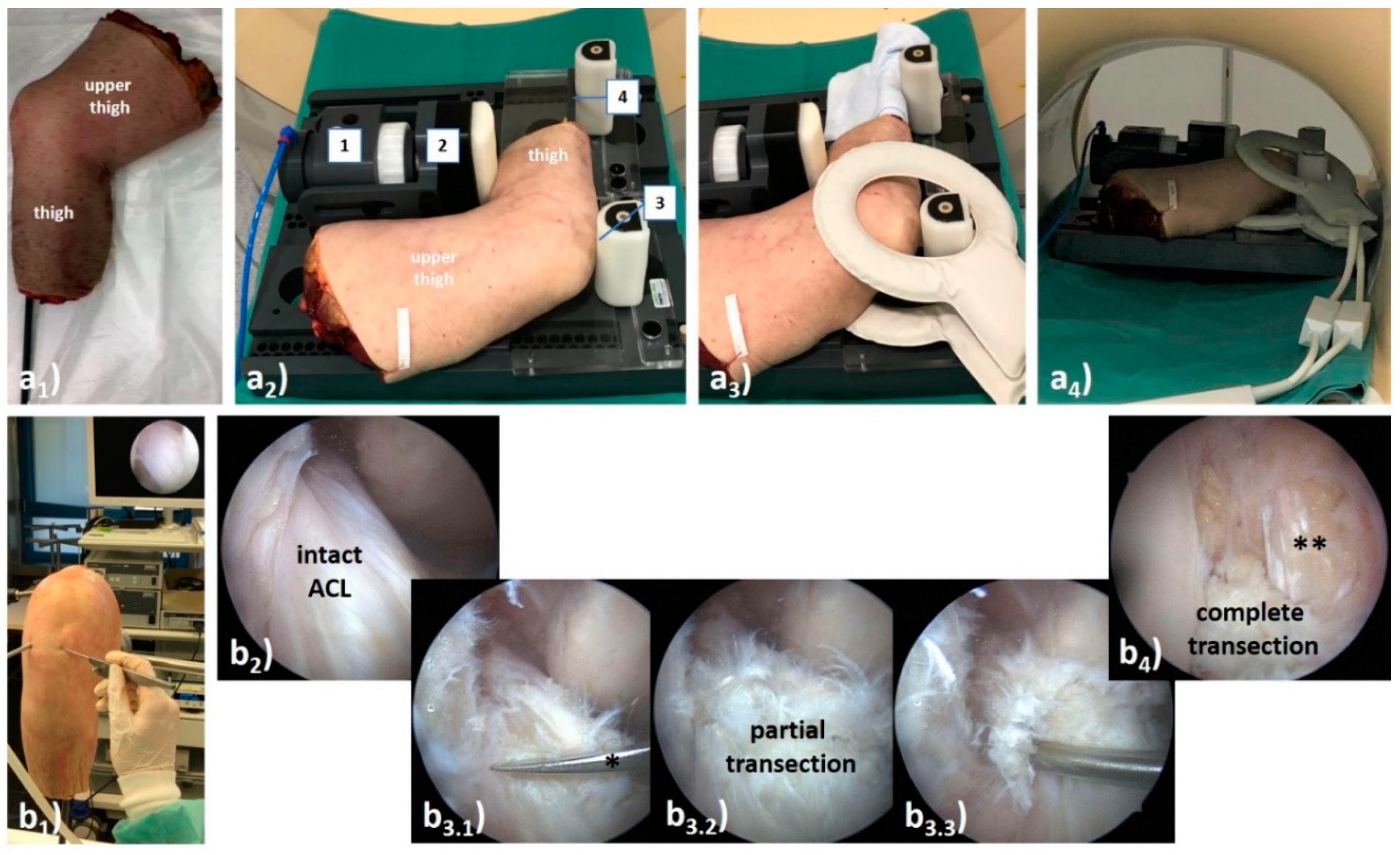
2.2. Loading Device and Human Knee Joint Specimens
2.3. MRI Studies
2.4. ACL Transection Model
2.5. Image Post-Processing and Analysis
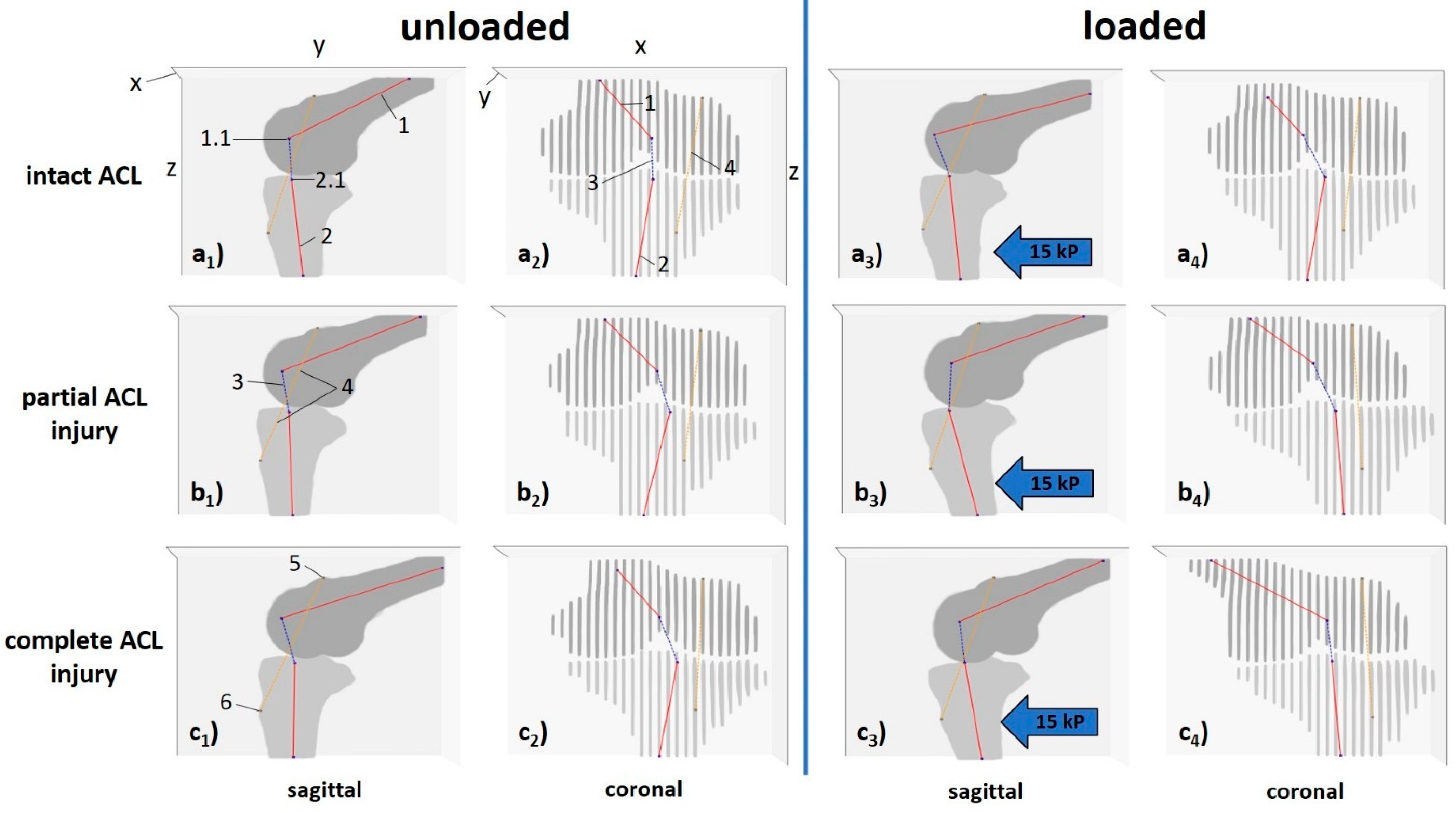
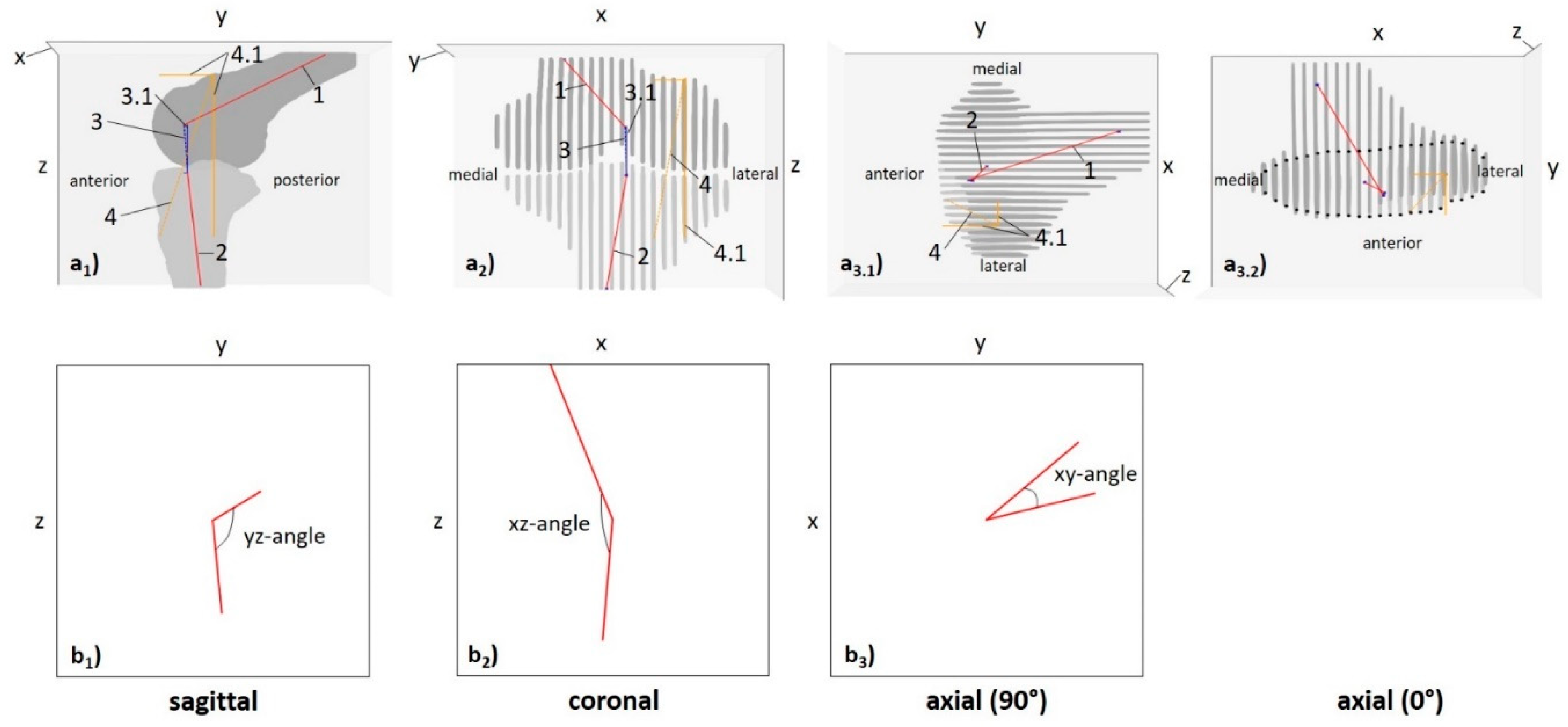
2.5.1. Computed 3D Measures
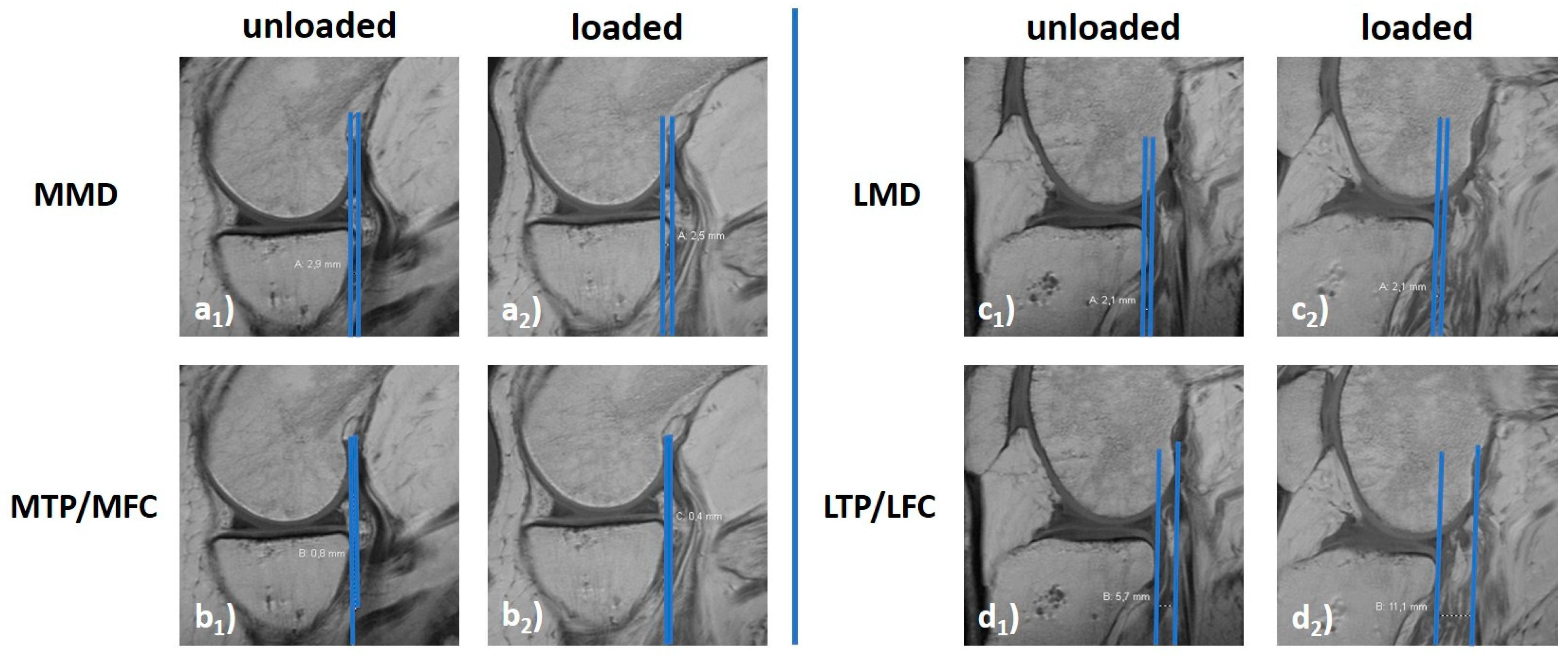
2.5.2. Manual 2D Reference Measures
2.6. Statistical Analysis
3. Results
4. Discussion
5. Conclusions
Supplementary Materials
Author Contributions
Funding
Institutional Review Board Statement
Informed Consent Statement
Data Availability Statement
Acknowledgments
Conflicts of Interest
References
- Majewski, M.; Susanne, H.; Klaus, S. Epidemiology of athletic knee injuries: A 10-year study. Knee 2006, 13, 184–188. [Google Scholar] [CrossRef]
- Bollen, S. Epidemiology of knee injuries: Diagnosis and triage. Br. J. Sports Med. 2000, 34, 227–228. [Google Scholar] [CrossRef] [Green Version]
- Granan, L.P.; Forssblad, M.; Lind, M.; Engebretsen, L. The Scandinavian ACL registries 2004–2007: Baseline epidemiology. Acta Orthop. 2009, 80, 563–567. [Google Scholar] [CrossRef] [PubMed] [Green Version]
- Shakoor, D.; Guermazi, A.; Kijowski, R.; Fritz, J.; Roemer, F.W.; Jalali-Farahani, S.; Demehri, S. Cruciate ligament injuries of the knee: A meta-analysis of the diagnostic performance of 3D MRI. J. Magn. Reson. Imaging 2019, 50, 1545–1560. [Google Scholar] [CrossRef]
- Chen, W.-T.; Shih, T.-F.; Tu, H.-Y.; Chen, R.-C.; Shau, W.-Y. Partial and complete tear of the anterior cruciate ligament: Direct and indirect MR signs. Acta Radiol. 2002, 43, 511–516. [Google Scholar] [PubMed]
- Umans, H.; Wimpfheimer, O.; Haramati, N.; Applbaum, Y.; Adler, M.; Bosco, J. Diagnosis of partial tears of the anterior cruciate ligament of the knee: Value of MR imaging. AJR Am. J. Roentgenol. 1995, 165, 893–897. [Google Scholar] [CrossRef] [PubMed]
- Lefevre, N.; Naouri, J.; Bohu, Y.; Klouche, S.; Herman, S. Partial tears of the anterior cruciate ligament: Diagnostic performance of isotropic three-dimensional fast spin echo (3D-FSE-Cube) MRI. Eur. J. Orthop. Surg. Traumatol. 2014, 24, 85–91. [Google Scholar] [CrossRef] [PubMed]
- Ng, A.W.; Griffith, J.F.; Hung, E.H.; Law, K.Y.; Yung, P.S. MRI diagnosis of ACL bundle tears: Value of oblique axial imaging. Skelet. Radiol. 2013, 42, 209–217. [Google Scholar] [CrossRef] [PubMed]
- Sonnery-Cottet, B.; Colombet, P. Partial tears of the anterior cruciate ligament. Orthop. Traumatol. Surg. Res. 2016, 102, S59–S67. [Google Scholar] [CrossRef]
- Ohashi, B.; Ward, J.; Araujo, P.; Kfuri, M.; Pereira, H.; Espregueira-Mendes, J.; Musahl, V. Partial Anterior Cruciate Ligament Ruptures: Knee laxity measurements and pivot shift. In Sports Injuries: Prevention, Diagnosis, Treatment and Rehabilitation; Springer: Berlin/Heidelberg, Germany, 2015; pp. 1245–1258. [Google Scholar]
- Noyes, F.; Mooar, L.; Moorman 3rd, C.; McGinniss, G. Partial tears of the anterior cruciate ligament. Progression to complete ligament deficiency. J. Bone Jt. Surg. Br. Vol. 1989, 71, 825–833. [Google Scholar] [CrossRef]
- Van Dyck, P.; De Smet, E.; Veryser, J.; Lambrecht, V.; Gielen, J.L.; Vanhoenacker, F.M.; Dossche, L.; Parizel, P.M. Partial tear of the anterior cruciate ligament of the knee: Injury patterns on MR imaging. Knee Surg. Sports Traumatol. Arthrosc. 2012, 20, 256–261. [Google Scholar] [CrossRef]
- Dejour, D.; Ntagiopoulos, P.G.; Saggin, P.R.; Panisset, J.-C. The diagnostic value of clinical tests, magnetic resonance imaging, and instrumented laxity in the differentiation of complete versus partial anterior cruciate ligament tears. Arthrosc. J. Arthrosc. Relat. Surg. 2013, 29, 491–499. [Google Scholar] [CrossRef]
- DeFranco, M.J.; Bach, B.R., Jr. A comprehensive review of partial anterior cruciate ligament tears. J. Bone Jt. Surg. Am. 2009, 91, 198–208. [Google Scholar] [CrossRef] [PubMed]
- Siebold, R.; Fu, F.H. Assessment and augmentation of symptomatic anteromedial or posterolateral bundle tears of the anterior cruciate ligament. Arthroscopy 2008, 24, 1289–1298. [Google Scholar] [CrossRef] [PubMed]
- Al-Dadah, O.; Shepstone, L.; Marshall, T.J.; Donell, S.T. Secondary signs on static stress MRI in anterior cruciate ligament rupture. Knee 2011, 18, 235–241. [Google Scholar] [CrossRef]
- Espregueira-Mendes, J.; Andrade, R.; Leal, A.; Pereira, H.; Skaf, A.; Rodrigues-Gomes, S.; Oliveira, J.M.; Reis, R.L.; Pereira, R. Global rotation has high sensitivity in ACL lesions within stress MRI. Knee Surg. Sports Traumatol. Arthrosc. 2017, 25, 2993–3003. [Google Scholar] [CrossRef] [PubMed]
- Temponi, E.F.; de Carvalho Júnior, L.H.; Sonnery-Cottet, B.; Chambat, P. Partial tearing of the anterior cruciate ligament: Diagnosis and treatment. Rev. Bras. Ortop. 2015, 50, 9–15. [Google Scholar] [CrossRef] [PubMed] [Green Version]
- James, E.W.; Williams, B.T.; LaPrade, R.F. Stress radiography for the diagnosis of knee ligament injuries: A systematic review. Clin. Orthop. Relat. Res. 2014, 472, 2644–2657. [Google Scholar] [CrossRef] [Green Version]
- Lee, Y.S.; Han, S.H.; Jo, J.; Kwak, K.-s.; Nha, K.W.; Kim, J.H. Comparison of 5 different methods for measuring stress radiographs to improve reproducibility during the evaluation of knee instability. Am. J. Sports Med. 2011, 39, 1275–1281. [Google Scholar] [CrossRef]
- Noh, J.H.; Nam, W.D.; Roh, Y.H. Anterior tibial displacement on preoperative stress radiography of ACL-injured knee depending on knee flexion angle. Knee Surg. Relat. Res. 2019, 31, 14. [Google Scholar] [CrossRef]
- Schneider, M.; Pinskerova, V.; Breusch, S.; Noe, V.; Freeman, M. Observations of normal and ACL-deficient knee joints after stress MRI. Der Orthop. 2006, 35, 337–346. [Google Scholar] [CrossRef] [PubMed]
- Espregueira-Mendes, J.; Pereira, H.; Sevivas, N.; Passos, C.; Vasconcelos, J.C.; Monteiro, A.; Oliveira, J.M.; Reis, R.L. Assessment of rotatory laxity in anterior cruciate ligament-deficient knees using magnetic resonance imaging with Porto-knee testing device. Knee Surg. Sports Traumatol. Arthrosc. 2012, 20, 671–678. [Google Scholar] [CrossRef] [Green Version]
- Said, O.; Schock, J.; Kramer, N.; Thuring, J.; Hitpass, L.; Schad, P.; Kuhl, C.; Abrar, D.; Truhn, D.; Nebelung, S. An MRI-compatible varus-valgus loading device for whole-knee joint functionality assessment based on compartmental compression: A proof-of-concept study. Magn. Reson. Mater. Phys. Biol. Med. 2020, 33, 839–854. [Google Scholar] [CrossRef] [PubMed]
- Yoon, J.P.; Yoo, J.H.; Chang, C.B.; Kim, S.J.; Choi, J.Y.; Yi, J.H.; Kim, T.K. Prediction of chronicity of anterior cruciate ligament tear using MRI findings. Clin. Orthop. Surg. 2013, 5, 19–25. [Google Scholar] [CrossRef]
- Yushkevich, P.A.; Piven, J.; Hazlett, H.C.; Smith, R.G.; Ho, S.; Gee, J.C.; Gerig, G. User-guided 3D active contour segmentation of anatomical structures: Significantly improved efficiency and reliability. NeuroImage 2006, 31, 1116–1128. [Google Scholar] [CrossRef] [Green Version]
- Lee, H.-J.; Park, Y.-B.; Kim, S.H. Diagnostic value of stress radiography and arthrometer measurement for anterior instability in anterior cruciate ligament injured knees at different knee flexion position. Arthrosc. J. Arthrosc. Relat. Surg. 2019, 35, 1721–1732. [Google Scholar] [CrossRef] [PubMed]
- Katz, J.W.; Fingeroth, R.J. The diagnostic accuracy of ruptures of the anterior cruciate ligament comparing the Lachman test, the anterior drawer sign, and the pivot shift test in acute and chronic knee injuries. Am. J. Sports Med. 1986, 14, 88–91. [Google Scholar] [CrossRef]
- Kondo, E.; Merican, A.M.; Yasuda, K.; Amis, A.A. Biomechanical analysis of knee laxity with isolated anteromedial or posterolateral bundle–deficient anterior cruciate ligament. Arthrosc. J. Arthrosc. Relat. Surg. 2014, 30, 335–343. [Google Scholar] [CrossRef]
- Loh, J.C.; Fukuda, Y.; Tsuda, E.; Steadman, R.J.; Fu, F.H.; Woo, S.L. Knee stability and graft function following anterior cruciate ligament reconstruction: Comparison between 11 o’clock and 10 o’clock femoral tunnel placement. Arthrosc. J. Arthrosc. Relat. Surg. 2003, 19, 297–304. [Google Scholar] [CrossRef]
- Zantop, T.; Herbort, M.; Raschke, M.J.; Fu, F.H.; Petersen, W. The Role of the Anteromedial and Posterolateral Bundles of the Anterior Cruciate Ligament in Anterior Tibial Translation and Internal Rotation. Am. J. Sports Med. 2007, 35, 223–227. [Google Scholar] [CrossRef]
- Vassalou, E.E.; Klontzas, M.E.; Kouvidis, G.K.; Matalliotaki, P.I.; Karantanas, A.H. Rotational knee laxity in anterior cruciate ligament deficiency: An additional secondary sign on MRI. Am. J. Roentgenol. 2016, 206, 151–154. [Google Scholar] [CrossRef]
- Polat, A.E.; Polat, B.; Gürpınar, T.; Sarı, E.; Çarkçı, E.; Erler, K. Tibial tubercle–trochlear groove (TT–TG) distance is a reliable measurement of increased rotational laxity in the knee with an anterior cruciate ligament injury. Knee 2020, 27, 1601–1607. [Google Scholar] [CrossRef]
- Mitchell, B.C.; Siow, M.Y.; Bastrom, T.; Bomar, J.D.; Pennock, A.T.; Parvaresh, K.; Edmonds, E.W. Coronal lateral collateral ligament sign: A novel magnetic resonance imaging sign for identifying anterior cruciate ligament–deficient knees in adolescents and summarizing the extent of anterior tibial translation and femorotibial internal rotation. Am. J. Sports Med. 2021, 49, 928–934. [Google Scholar] [CrossRef] [PubMed]
- Panisset, J.-C.; Ntagiopoulos, P.-G.; Saggin, P.; Dejour, D. A comparison of Telos™ stress radiography versus Rolimeter™ in the diagnosis of different patterns of anterior cruciate ligament tears. Orthop. Traumatol. Surg. Res. 2012, 98, 751–758. [Google Scholar] [CrossRef] [Green Version]
- Garces, G.; Perdomo, E.; Guerra, A.; Cabrera-Bonilla, R. Stress radiography in the diagnosis of anterior cruciate ligament deficiency. Int. Orthop. 1995, 19, 86–88. [Google Scholar] [CrossRef] [PubMed]
- Rijke, A.M.; Tegtmeyer, C.; Weiland, D.; McCue, F., 3rd. Stress examination of the cruciate ligaments: A radiologic Lachman test. Radiology 1987, 165, 867–869. [Google Scholar] [CrossRef] [PubMed]
- Lansdown, D.A.; Riff, A.J.; Meadows, M.; Yanke, A.B.; Bach, B.R., Jr. What factors influence the biomechanical properties of allograft tissue for ACL reconstruction? A systematic review. Clin. Orthop. Relat. Res. 2017, 475, 2412–2426. [Google Scholar] [CrossRef]


| Sequence Parameters | PDW fs | PDW fs | PDW fs | T1 | T2 |
|---|---|---|---|---|---|
| Sequence type | 2D TSE | 2D TSE | 2D TSE | 2D TSE | 2D TSE |
| Orientation | cor | ax | sag | sag | parasag & parax (*) |
| Type of fat saturation | SPAIR | SPAIR | SPAIR | n/a | n/a |
| Repetition time [ms] | 4495 | 4776 | 4928 | 671 | 3000 |
| Echo time [ms] | 30 | 30 | 30 | 9 | 80 |
| Turbo spin-echo factor | 13 | 13 | 15 | 3 | 14 |
| Field of view [mm] | 160 × 160 | 160 × 160 | 160 × 160 | 160 × 160 | 160 × 160 |
| Acquisition matrix [pixels] | 400 × 300 | 400 × 312 | 352 × 255 | 368 × 317 | 352 × 295 |
| Reconstruction matrix [pixels] | 512 × 512 | 512 × 512 | 512 × 512 | 448 × 448 | 512 × 512 |
| Scan percentage [%] | 79.4 | 79.4 | 79.3 | 86.1 | 85.0 |
| Flip angle [°] | 90 | 90 | 90 | 90 | 90 |
| Number of signal averages [n] | 1 | 1 | 1 | 1 | 1 |
| Slices [n] | 31 | 33 | 26 | 30 | 7 |
| Slice thickness/gap [mm] | 3.0/0.3 | 3.0/0.3 | 3.0/0.3 | 3.0/0.3 | 3.0/0.3 |
| Duration [min:sec] | 04:39 | 03:59 | 03:27 | 06:40 | 07:30 |
| Category of Measure | Measure [Unit] | Description of Measure | Intact | Partial ACL Deficiency | Complete ACL Deficiency | p-Value | |||
|---|---|---|---|---|---|---|---|---|---|
| δ0 | δ1 | δ0 | δ1 | δ0 | δ1 | ||||
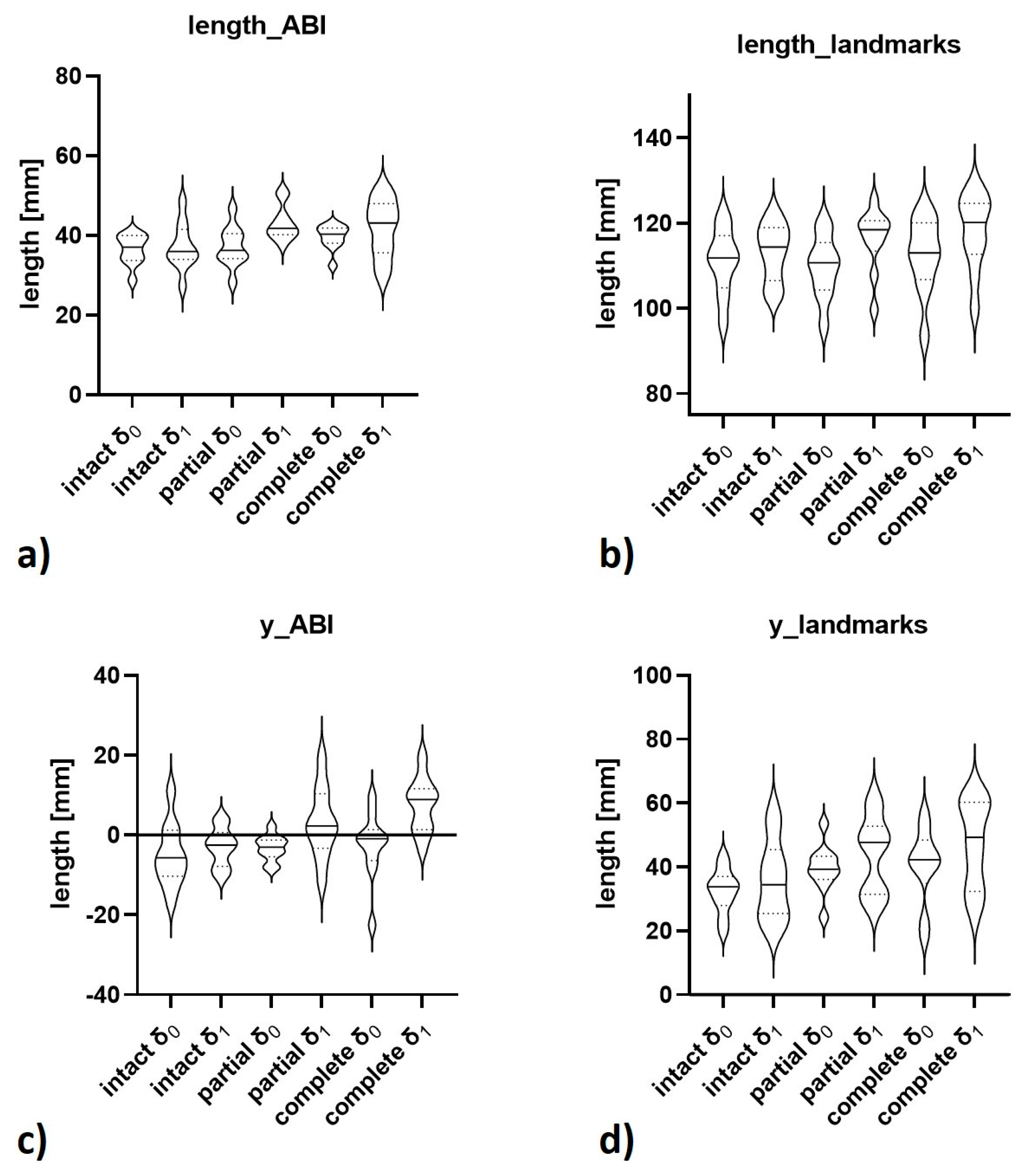
| Computed 3D Measures | length_ABI [mm] | length of vector_ABI | 36.4 ± 3.8 | 37.2 ± 5.9 | 37.2 ± 5.1 | 43.1 ± 4.4 | 39.6 ± 3.1 | 41.8 ± 7.3 | <0.001 [1] |
| x_ABI [mm] | projected length of vector_ABI along x-axis (mediolateral) | −2.3 ± 8.7 | −1.8 ± 4.7 | −3.5 ± 4.6 | −5.4 ± 6.0 | −5.0 ± 6.5 | −2.0 ± 6.4 | 0.579 | |
| y_ABI [mm] | projected length of vector_ABI along y-axis (anteroposterior) | −5.0 ± 7.9 | −3.0 ± 4.9 | −3.3 ± 3.2 | 3.1 ± 8.9 | −2.6 ± 8.6 | 7.6 ± 6.8 | <0.001 [2] | |
| z_ABI [mm] | projected length of vector_ABI along z-axis (craniocaudal) | 34.0 ± 5.5 | 36.5 ± 5.9 | 36.5 ± 4.9 | 41.4 ± 4.1 | 37.3 ± 7.6 | 40.2 ± 6.4 | <0.001 [3] | |
| length_landmarks [mm] | length of vector_landmarks | 110.9 ± 7.8 | 113.2 ± 6.8 | 109.7 ± 7.3 | 116.3 ± 7.4 | 112.4 ± 8.9 | 118.0 ± 8.9 | <0.001 [4] | |
| x_landmarks [mm] | projected length of vector_landmarks along x-axis (mediolateral) | 7.3 ± 5.1 | 7.5 ± 3.7 | 5.2 ± 3.7 | 5.4 ± 4.4 | 7.3 ± 6.4 | 5.0 ± 3.6 | 0.644 | |
| y_landmarks [mm] | projected length of vector_landmarks along y-axis (anteroposterior) | 32.5 ± 7.0 | 35.8 ± 12.6 | 39.5 ± 7.5 | 43.9 ± 12.1 | 40.5 ± 11.9 | 47.3 ± 13.7 | 0.003 [5] | |
| z_landmarks [mm] | projected length of vector_landmarks along z-axis (craniocaudal) | 105.5 ± 7.1 | 106.4 ± 5.8 | 102.0 ± 5.7 | 106.9 ± 7.7 | 103.9 ± 7.6 | 107.3 ± 7.3 | 0.110 | |
| xz-angle [°] | projected angle of central bone axes on xz-plane (coronal) | 143.6 ± 15.0 | 140.7 ± 24.7 | 138.0 ± 15.2 | 130.8 ± 22.1 | 137.0 ± 28.1 | 117.5 ± 18.6 | 0.016 | |
| yz-angle [°] | projected angle of central bone axes on yz-plane (sagittal) | 109.5 ± 11.7 | 103.3 ± 9.7 | 108.8 ± 10.3 | 98.0 ± 5.1 | 101.5 ± 12.1 | 101.2 ± 8.5 | <0.001 [6] | |
| xy-angle [°] | projected angle of central bone axes on xy-plane (axial) | 34.9 ± 21.4 | 29.5 ± 25.6 | 39.0 ± 29.6 | 25.5 ± 16.3 | 28.7 ± 23.7 | 26.2 ± 20.6 | 0.723 | |
| Manual 2D Measures | LMD [mm] | distance between posterior horn (lateral meniscus) and posterior margin (tibial plateau) | 4.1 ± 1.6 | 0.9 ± 2.1 | 4.0 ± 2.9 | 0.1 ± 2.1 | 2.7 ± 2.7 | −0.2 ± 3.0 | 0.001 [7] |
| LTP/LFC [mm] | distance between femoral condyle (lateral) and posterior margin (tibial plateau) | −3.0 ± 2.7 | −6.0 ± 5.1 | −4.0 ± 3.8 | −9.9 ± 3.6 | −5.4 ± 3.8 | −10.8 ± 4.1 | 0.302 | |
| MMD [mm] | distance between posterior horn (medial meniscus) and posterior margin (tibial plateau) | 3.7 ± 1.4 | 1.8 ± 2.4 | 3.1 ± 2.2 | 0.3 ± 1.7 | 1.8 ± 1.0 | −0.3 ± 1.3 | <0.001 [8] | |
| MTP/MFC [mm] | distance between femoral condyle (medial) and posterior margin (tibial plateau) | 1.2 ± 1.8 | −0.7 ± 3.4 | 0.3 ± 4.3 | −2.4 ± 2.4 | −1.4 ± 2.0 | −4.6 ± 2.4 | <0.001 [9] | |
Publisher’s Note: MDPI stays neutral with regard to jurisdictional claims in published maps and institutional affiliations. |
© 2021 by the authors. Licensee MDPI, Basel, Switzerland. This article is an open access article distributed under the terms and conditions of the Creative Commons Attribution (CC BY) license (https://creativecommons.org/licenses/by/4.0/).
Share and Cite
Winkelmeyer, E.-M.; Schock, J.; Wollschläger, L.M.; Schad, P.; Huppertz, M.S.; Kotowski, N.; Prescher, A.; Kuhl, C.; Truhn, D.; Nebelung, S. Seeing Beyond Morphology-Standardized Stress MRI to Assess Human Knee Joint Instability. Diagnostics 2021, 11, 1035. https://doi.org/10.3390/diagnostics11061035
Winkelmeyer E-M, Schock J, Wollschläger LM, Schad P, Huppertz MS, Kotowski N, Prescher A, Kuhl C, Truhn D, Nebelung S. Seeing Beyond Morphology-Standardized Stress MRI to Assess Human Knee Joint Instability. Diagnostics. 2021; 11(6):1035. https://doi.org/10.3390/diagnostics11061035
Chicago/Turabian StyleWinkelmeyer, Eva-Maria, Justus Schock, Lena Marie Wollschläger, Philipp Schad, Marc Sebastian Huppertz, Niklas Kotowski, Andreas Prescher, Christiane Kuhl, Daniel Truhn, and Sven Nebelung. 2021. "Seeing Beyond Morphology-Standardized Stress MRI to Assess Human Knee Joint Instability" Diagnostics 11, no. 6: 1035. https://doi.org/10.3390/diagnostics11061035