1. Introduction
Stroke due to a large vessel occlusion in the posterior circulation accounts for approximately 1% [
1,
2] of all cases of acute ischemic stroke and is associated with poor outcome [
3]. Posterior circulation stroke (PCS) may have an acute onset or a progressive and stuttering onset, and may produce symptoms that are not typically associated with anterior stroke, such as vertigo and nausea [
1]. Therefore, PCS is associated with a higher chance of misinterpretation and under-diagnosis in clinical practice than anterior circulation stroke (ACS) [
4,
5], which has resulted in long delays in door-to-needle times of patients suffering from a PCS compared to patients suffering from an ACS [
6,
7]. Reducing time from symptom onset to treatment may improve the outcome of patients suffering from a PCS who are treated with intravenous alteplase treatment and/or endovascular treatment [
8,
9,
10].
Localizing an occluding thrombus causing PCS on radiological imaging is not a problem for expert neuro-radiologists and can be done quickly [
11]. However, timely access to the services of an expert neuro-radiologist may not be possible in primary stroke centers because of the limited number of available neuro-radiologists. Automated localization of PCS may help to avoid misinterpretation in the case of a PCS. In addition to localization, segmentation of the thrombus would allow for automatic quantification of thrombus volume. Thrombus volume was previously reported to be negatively associated with recanalization and a higher likelihood of poor functional outcome [
12,
13].
Recently proposed methods for the automated localization and segmentation of thrombi in stroke patients make use of convolutional neural networks (CNNs) [
14,
15,
16]. Training CNNs requires imaging data from a large number of patients to reach an acceptable localization accuracy. For anterior circulation stroke, data from large numbers of patients are available even in single medical centers. However, data from patients suffering from a PCS are scarce.
As opposed to thrombi in patients with an ACS, thrombi in patients with a PCS occur in a more limited area around the brainstem. This characteristic can be used to improve the performance of a CNN-based thrombus localization and segmentation method. A CNN can learn how to center a moving volume-of-interest (VOI) on the brainstem and evaluate only locations with a high likelihood of a thrombus. We hypothesize that tracking the brainstem with a small VOI improves the localization and segmentation of thrombi in the posterior circulation. In addition, we hypothesize that by removing small, segmented thrombi, the number of false positive thrombus localizations can be reduced.
In this study, we aim to develop and evaluate the first automatic CNN-based method for thrombus localization and segmentation on baseline on non-contrast CT (NCCT) and CT angiography (CTA) in patients suffering from a PCS.
2. Materials and Methods
2.1. Materials
The data used in this study were obtained from a prospective and nationwide observational study on endovascular treatment in the Netherlands (the MR CLEAN Registry [
17]). The data were collected in 16 centers that performed endovascular treatment in the Netherlands between March 2014 and January 2019. The dataset used in our study included all patients from the MR CLEAN Registry that suffered from a PCS and consisted of NCCT and CTA scans from 268 patients. Hence, patients were also included if they suffered from an anterior circulation stroke (three patients) or a subarachnoid hemorrhage (one patient) in addition to a PCS. Patients were excluded if no baseline CTA was available, the scan quality was too low, registration of the NCCT to the CTA was unsuccessful, or if the patient had a non-occlusive thrombus or dissection. The Medical Ethics Committee of the Erasmus University Medical Center in Rotterdam, the Netherlands, approved the MR CLEAN Registry (MEC-2014-235). In addition, the institutional review board of each participating center approved the MR CLEAN research protocol.
2.2. Reference Annotations
Two types of annotations were made: reference thrombus segmentations, and annotations of the reference path, which runs through the structures of the brainstem. The reference segmentations of the thrombi were obtained by manual annotation. One trained observer (RZ) manually segmented the thrombi, and the second observer (AAEB) corrected the segmentations if necessary. A window width of 30 Hounsfield units (HU) and a center level of 35 HU was used for the NCCT scan, and a window width of 600 HU and a center level of 300 HU was used for the CTA scan. Annotations were made using ITK-Snap. For each patient, a case record form was available from an imaging core lab, which indicated the location of the occlusion and whether a hyperdense artery sign (HAS) was visible on the NCCT. The information about the location of the occlusion was used to guide the manual annotation. If the patient had a HAS, the NCCT was used to create the reference segmentation. Otherwise, the absence of arterial filling on the CTA was used to create the reference segmentation.
The reference path through the brainstem was annotated by one trained observer (RZ). The path started in the spinal cord, continued through the medulla oblongata, pons and midbrain. The reference path was marked by annotating a single voxel per axial slice in ITK Snap.
2.3. Preprocessing
To limit the size of the scan, all slices 25 cm below the top of the skull were excluded. Next, to align the anatomical structures in the CTA to those in the NCCT, the CTAs were registered to the NCCT by using rigid transformations. Finally, the voxel intensities were clipped between −100 and 200 HU and normalized between minus one and one. The preprocessing was done using SimpleITK and python 3.8.5.
2.4. CNNs for Automatic Posterior Circulation Thrombus Localization and Segmentation
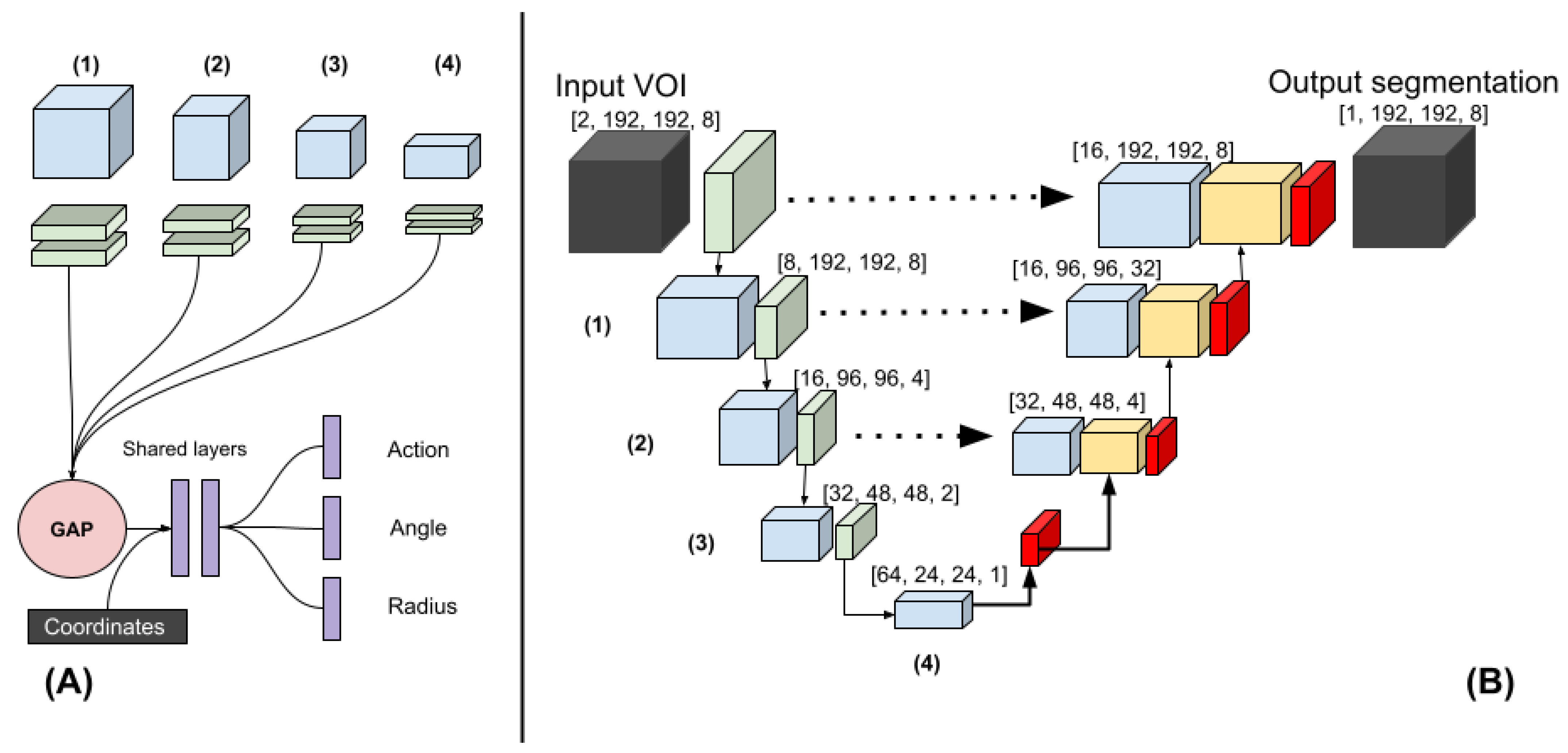
Existing deep-learning methods result in false positive localization and segmentation if they are used on small objects. We developed a method to reduce the number of false positive localizations by restricting the VOI to a region that included the brain stem, which was most likely to contain a thrombus in patients suffering from a PCS. To restrict the VOI to the brainstem, the method had to learn how to move the VOI towards the brainstem on an axial slice. The movement from the center of the VOI at a given location was parameterized as a circle with a radius and an angle (polar coordinates). The method learned to regress these polar coordinates and was named polar-UNet. In addition to regressing the polar coordinates, polar-UNet classified what action should be taken at each step: to move the VOI within the current axial slice, segment and move up one axial slice, or to stop the inference procedure.
The architecture of the regression and classification heads of the polar-UNet is shown in
Figure 1A. To create the polar-UNet, the regression and classification head were added to the down-sampling path of the baseline UNet (BL-UNet), which is shown in
Figure 1B. Features were extracted at four levels of the down-sampling path. These features were input into four separate convolutional layers and global average-pooled. Next, the extracted features were concatenated with the relative coordinates of the VOI in the scan volume and input into two shared fully connected layers, which consisted of 256 neurons each. The output of the shared layer was passed to the individual network heads, which regressed either the angle or the radius, or classified the action. The angle regression head used a TanH activation, the radius regression head used a sigmoid activation, and the action classification head used the softmax activation function in the output layer. Finally, polar-UNet also had the same up-sampling path as BL-UNet.
The BL-UNet was inspired by U-Net [
18] and consisted of 3D ResNet [
19] blocks. The down-sampling path started with two convolutional layers, which consisted of a kernel size of three and a stride of one. It was followed by a max-pooling operation with a kernel size and stride of two. Subsequently, three down-sampling blocks, which consisted of a 3D ResNet layer each, were added. The first two blocks were followed by a max-pooling layer with a stride and pooling size of two. The up-sampling path started with a transposed convolution. Next, two up-sampling blocks, which consisted of a ResNet block followed by a transposed convolution, were added. Each transposed convolution had a stride of two and a kernel size of three. The features of the down-sampling path were concatenated with the features in the up-sampling path. The up-sampling path was followed by a three-by-three convolution and a one-by-one convolution. During inference, BL-UNet was applied to a non-overlapping grid of VOIs extracted from the entirety of each scan. The CNNs were implemented using Pytorch 1.5.1 [
20].
2.5. Experimental Setup
The BL-UNet was randomly initialized and trained on VOIs sampled from the scan volumes. To ensure the data contained sufficient positive examples, 40 percent of the sampled VOIs contained a thrombus. The up-sampling and down-sampling paths of the polar-UNet were initialized by reusing the weights obtained by the pre-trained BL-UNet and were not updated during training. The BL-UNet used group normalization with 4 groups, the ReLU activation, a batch size of 32, a cyclical learning rate schedule, the Adam optimizer and a weight decay of . The BL-UNet was trained for 300 epochs with 148 iterations per epoch.
The polar-UNet applied batch-normalization to the layers that were updated during training and used a batch size of 128. The focal loss function was used for the segmentation and classification tasks, and the
loss [
21] for the regression tasks. The polar-UNet was trained for 100 epochs with 148 iterations per epoch. Both CNNs used a maximum learning rate of
, a minimum learning rate of
, and the weight decay was set to
. The learning rate was linearly increased to the maximum value in 300 iterations and decreased to the minimum value in 300 iterations.
The polar coordinate reference values that were needed to move the VOI to the area around the brainstem were calculated using the reference path. The angle reference value was calculated as the angle between the coordinates of the center of the VOI and the coordinates of the reference path on the same axial slice. To allow for easier optimization, the angle reference values were normalized between 0 and 2. The radius reference value indicated the step size that the VOI had to be moved to minimize the Euclidean distance between the center of the VOI and the reference path on the same axial slice. The radius was limited to the width of the VOI and normalized between 0 and 1 to allow for easier optimization.
The inference procedure of the polar-UNet is shown in the
Supplementary Materials Algorithm S1. We initialized the VOI at the center of the most caudal axial slice in the scan. Per axial slice, the VOI could only be moved within the axial slice 10 times before the VOI location was moved up by one axial slice. If the VOI moved out of the bounds of the volume, the VOI location was moved up by one slice and reset to the center of the axial slice.
Data augmentation was applied during training. The axial slices in the scan volumes were rotated at an angle between minus ten and ten degrees and, with a probability of 0.5, were flipped. Furthermore, the scan volumes were magnified by a factor between 0.9 and 1.1 and translated in the axial plane by a maximum of 80 voxels. Polar coordinates reference values were updated accordingly. The sampled VOIs had dimensions of 192 × 192 × 8.
We used stratified five-fold cross-validation to evaluate the performance of the CNN architectures. The hyper-parameters used in our study were found by evaluating multiple sets of hyper-parameters on the first fold and selecting the ones with the highest testing performance. To prevent inflation of the results due to the first fold being used to find the optimal hyper-parameters, this fold was excluded from the evaluation.
To improve the localization precision of the CNNs, only connected components larger than 0.065 mL were included in further analyses. We refer to this step as volume-based removal (VBR).
2.6. Evaluation
To evaluate the localization performance of our models, we calculated the thrombus localization precision and recall. Hence, the number of true positive (TP), false positive (FP), and false negative (FN) localizations had to be calculated. To calculate the TP, FP, and FN localizations, the segmentation maps had to be divided into individual connected regions. Thus, a connected-components analysis was run on the automatically created and manually annotated segmentations. If two connected components from the manually annotated segmentation and the corresponding automatically created segmentation had ten percent or more of their voxels overlapping, this was counted as a TP localization. If a connected component from the automatically created segmentation had less than ten percent overlap with a connected component from the manually annotated segmentation it was counted as a FP localization. If a connected component from the manually annotated segmentation did not have more than ten percent overlap with any of the connected components from the automatically created segmentation, it was counted as a FN.
The intra-class correlation coefficient (ICC) was used to evaluate the agreement between the volume derived from the automatically and manually segmented thrombi. We included the 95% confidence interval (95% CI) in our analysis. Furthermore, we performed a Bland-Altman analysis to evaluate the bias and limits of agreement of the volume measurements. We tested whether the ICC of the automated segmentations created by the two CNN architectures with and without VBR differed significantly by using Fishers r to z transformation.
The segmentation overlap of the CNNs was evaluated by calculating the Dice coefficient between the reference and the automatic segmentation. If no thrombus was visible in the scan, the Dice coefficient would always equal zero and would always deflate the results artificially. Hence, patients with no visible thrombus in the scan were excluded from the analysis of the Dice coefficient.
The obtained metrics were tested for normality with Shapiro-Wilk tests. If the obtained metrics followed a normal distribution, paired t-tests were used for comparison, otherwise Wilcoxon rank-sum tests were used. A Bonferroni correction was applied to P-values to correct for family-wise error. Finally, thrombi in the posterior circulation most commonly occur in the basilar artery. Therefore, we evaluated whether thrombus location influenced true positive thrombus localization, volume agreement, and segmentation overlap. Thrombus location was obtained from the case report file of each patient. The Python library Pingouin, version 0.3.1 was used for all statistical testing.
3. Results
In 185 out of 187 scans (99%) a thrombus was visible and was manually annotated. After exclusion of the patients in the test set of the first fold, due to this fold being used for hyper-parameter optimization, 149 scans were left to evaluate the results on.
The thrombus localization recall varied between 129 (69%) and 146 (82%). The thrombus localization recall before and after VBR for the BL-UNet and polar-UNet is shown in
Table 1. Overall, the Polar-UNet improved the thrombus localization recall over BL-UNet, and VBR reduced the thrombus localization recall of both CNNs.
The thrombus localization precision before and after VBR for the BL-UNet and polar-UNet is shown in
Table 1. In all cases, Polar-UNet improved the thrombus localization precision over the BL-UNet, and VBR improved the thrombus localization precision of both CNNs (
Figure 2). However, for all cases the thrombus localization precision is low with an overall maximum of 62%.
The median thrombus volume was 0.15 (IQR: 0.07–0.34) mL. The ICC for the volume agreement of the BL-UNet and Polar-UNet without VBR were 0.38 (95% CI: 0.23–0.51) and 0.4 (95% CI: 0.25–0.53). With VBR, the ICCs for the volume agreement of the BL-UNet and Polar-UNet were both 0.41 (95% CI: 0.27–0.54). There was no statistically significant difference between the volumetric agreement of the various methods. The Bland-Altman analysis for each of the CNNs resulted in biases ranging from −0.06 mL for the Polar-UNet without VBR to 0.06 mL for the BL-UNet with VBR. The LoAs were the smallest for the BL-UNet with VBR, ranging from −0.64 to 0.77 mL. The LoAs were largest for the Polar-UNet without VBR, ranging from −0.83 to 0.71 mL. The bias and LoAs for the volume analysis are shown in the
Supplementary Materials Table S3, and the Bland-Altman results are shown in
Figure 3.
The Dice coefficients for the automated thrombus segmentation are shown in
Table 1. The results of the Wilcoxon rank-sum test are shown in the
Supplementary Materials Table S2. The results show that the Polar-UNet with VBR results in a statistically significantly larger Dice coefficient than the other methods. Furthermore, the Polar-UNet without VBR results in a significantly greater Dice coefficient than the BL-UNet with or without VBR.
4. Discussion
In this study we have presented the first CNN-based method to segment and localize thrombi in patients suffering from PCS. The restriction of the VOI to areas in the vicinity of the brainstem improved the segmentation overlap and thrombus localization precision and recall over the baseline method. The VBR of small objects improved the thrombus localization precision of our method but reduced the recall. Regardless of whether VBR of small objects is applied, the bias of the automated volume quantifications is small, but the limits of agreement are large. Finally, there is room to improve the methods volume agreement and segmentation overlap.
Our study is the first to address the automated localization and segmentation of thrombi in the posterior circulation on CTA and NCCT. Prior work has focused on identifying scans with a large vessel occlusion (LVO) in the anterior circulation on a single-phase [
22,
23] and multi-phase [
14,
24] CTA. Two studies included patients suffering from both types of stroke, either in the posterior or anterior circulation [
14,
25]. However, a limitation is that not all studies report results specific to the posterior stroke patient group [
14]. Another limitation of prior work is that the thrombus is not localized, nor is it segmented. Only the presence or absence of an LVO in a scan is indicated.
Other work aimed to localize or segment thrombi on NCCT scans of patients suffering from either anterior or posterior circulation stroke [
15,
26,
27]. One study used feature extraction and a random forest classifier [
27]. This study did not mention the location of the thrombi in their dataset. Other work has used deep learning to localize or segment thrombi on NCCT scans of patients in the anterior circulation [
15,
26]. A key feature of these methods is that a comparison between hemispheres was made to improve localization or segmentation performance. A comparison between hemispheres has no added value to PCS thrombus localization and segmentation, because of the absence of lateral symmetry of the basilar artery.
Our study has several limitations. First, our method is not accurate at localizing and segmenting thrombi in the vertebral and posterior cerebral artery. This is likely because of the rareness of thrombi in these sections. Hence, data from few patients with occlusions in these regions were available to train our method on. In contrast, our method does achieve a good localization precision and a reasonable segmentation accuracy for thrombi in the basilar artery, which is the most common location for PCS. Second, our data was annotated by one trained observer. Hence, the inter-observer agreement could not be assessed. However, the manual segmentations were verified and corrected by another experienced observer. Third, the method achieved a low volumetric agreement and segmentation overlap between the manually and automatically segmented thrombi. Still, the volumetric agreement is similar to those reported in a study that focuses on thrombus segmentation and localization in the anterior circulation [
15]. This is despite our method not being able to use lateral symmetry information, as was done by methods for anterior stroke localization and segmentation. Furthermore, the low Dice coefficient can be explained by the small size of the thrombi. For small object segmentation, the Dice coefficient is over-sensitive to small errors [
28]. Fourth, manual segmentation of thrombi in patients without a HAS and with poor collateral status on single phase CTA leads to an overestimation of thrombus length [
29]. The overestimation of thrombus length is caused by a delayed contrast arrival. Hence, our method may, just like manual segmentations, overestimate the true length of the occluding thrombus. Fifth, since there were no additional large datasets with patients with posterior stroke available, our method lacks validation on an external dataset. Thus, results may vary when our algorithm is trained on or applied to other datasets. However, the data in our study were collected from sixteen different centers. Our algorithm was nonetheless evaluated on a heterogeneous set of scans. As more image data of patients with posterior stroke become available, our method may be improved and validated by including this image data.
A valuable application of deep learning is to automate time-critical and labor-intensive tasks such as the localization and segmentation of small objects in radiological imaging. Our study has shown that for small object segmentation and localization, a standard deep-learning-based segmentation method would result in large amounts of false positives. In this study we have presented an approach that combines restricting the segmentation and localization to the region in which the occlusion occurs, and excluding small objects. We have shown that this combination reduces the number of false positives.
The automated posterior thrombus localization and segmentation method is the first step towards a method that allows associations between thrombus characteristics, such as thrombus volume and length, and PCS outcome to be easily studied in clinical trials.


 ,
, 


