Figure 1.
A normal fundus image (left) and a representative DR fundus image with multiple types of lesions (right).
Figure 1.
A normal fundus image (left) and a representative DR fundus image with multiple types of lesions (right).
Figure 2.
Components analyzed in our deep learning-based DR grading framework. The evaluation process of a framework can be divided into two parts: training (top) and testing (bottom). In the training phase, we first fix the architecture of the selected network (ResNet-50). Then, we examine a collection of designs with respect to the training setting including preprocessing (image resizing and enhancement), training strategies (compositions of data augmentation (DA) and sampling strategies), and optimization configurations (objective functions and learning rate (LR) schedules). In the testing phase, we apply the same preprocessing as in the training phase and employ paired feature fusion to make use of the correlation between the two eyes (the training step of the fusion network is omitted in this figure). Then, we select the best ensemble method for the final prediction.
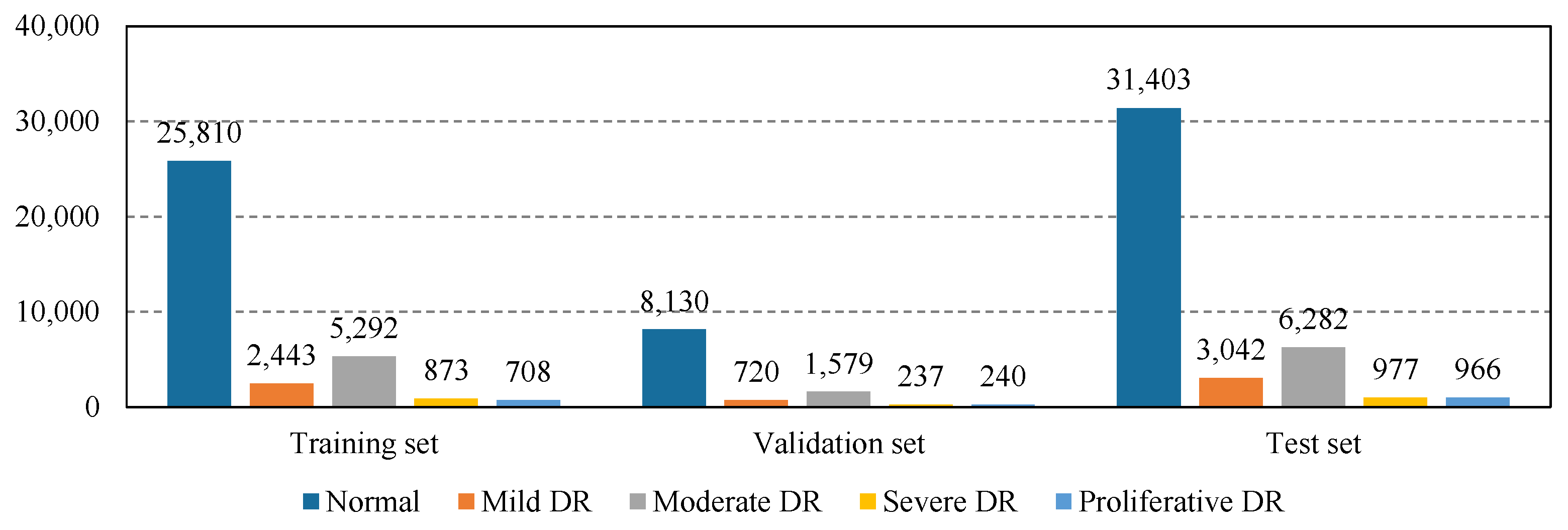
Figure 3.
The imbalanced class distribution of EyePACS.
Figure 3.
The imbalanced class distribution of EyePACS.
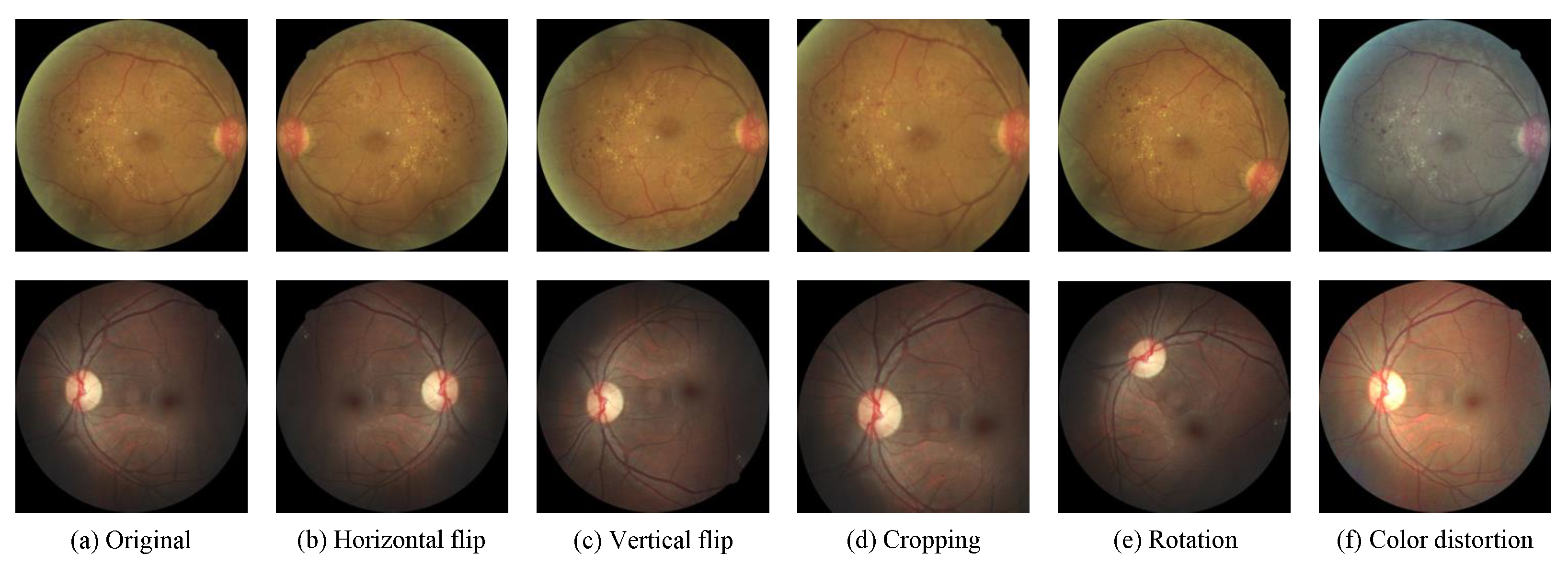
Figure 4.
Illustration of common data augmentation operations.
Figure 4.
Illustration of common data augmentation operations.
Figure 5.
Representative enhanced fundus images using Graham processing and CLAHE.
Figure 5.
Representative enhanced fundus images using Graham processing and CLAHE.
Figure 6.
Representative eye pairs with different quality of the left and right fields.
Figure 6.
Representative eye pairs with different quality of the left and right fields.
Figure 7.
Confusion matrices from models, respectively, using the cross-entropy loss and the MSE loss as the objective function. All values in the confusion matrices are normalized.
Figure 7.
Confusion matrices from models, respectively, using the cross-entropy loss and the MSE loss as the objective function. All values in the confusion matrices are normalized.
Figure 8.
The performance of models using different sampling strategies for training. The dotted red line represents the best validation Kappa among these four experiments, which is achieved by instance-balanced sampling.
Figure 8.
The performance of models using different sampling strategies for training. The dotted red line represents the best validation Kappa among these four experiments, which is achieved by instance-balanced sampling.
Figure 9.
Box plots of the test Kappa of all experiments in this work. The experiments in each column are set up based on the best model considering all its left components. DA and PFF denote the experiment results of different compositions of data augmentation and applying paired feature fusion or not.
Figure 10.
Visualization results from GradCAM. Representative eye pairs of four grades (mild DR, moderate DR, severe DR, and proliferate DR) are presented from top to bottom. The intensity of the heatmap indicates the importance of each pixel in the corresponding image for making the prediction.
Figure 10.
Visualization results from GradCAM. Representative eye pairs of four grades (mild DR, moderate DR, severe DR, and proliferate DR) are presented from top to bottom. The intensity of the heatmap indicates the importance of each pixel in the corresponding image for making the prediction.
Table 1.
DR grading performance with different input resolutions on EyePACS. Two GPUs are used to train the model with input resolution due to the CUDA memory limitation.
Table 1.
DR grading performance with different input resolutions on EyePACS. Two GPUs are used to train the model with input resolution due to the CUDA memory limitation.
| Resolution | Training Time | FLOPs | Validation Kappa | Test Kappa |
|---|
| 1 h 54 m | 1.35 G | 0.6535 | 0.6388 |
| 2 h 19 m | 5.40 G | 0.7563 | 0.7435 |
| 5 h 16 m | 21.61 G | 0.8054 | 0.8032 |
| 11 h 15 m | 48.63 G | 0.8176 | 0.8137 |
| 11 h 46 m (2 GPUs) | 86.45 G | 0.8187 | 0.8164 |
Table 2.
DR grading performance of models using different objective functions on EyePACS. is empirically set to be 2 for the focal loss.
Table 2.
DR grading performance of models using different objective functions on EyePACS. is empirically set to be 2 for the focal loss.
| Loss | Validation Kappa | Test Kappa |
|---|
| Cross Entropy (CE) | 0.8054 | 0.8032 |
| Focal ( = 2) | 0.8079 | 0.8059 |
| Kappa | 0.7818 | 0.7775 |
| Kappa + CE | 0.8047 | 0.8050 |
| MAE | 0.7655 | 0.7679 |
| Smooth L1 | 0.8094 | 0.8117 |
| MSE | 0.8207 | 0.8235 |
Table 3.
DR grading performance of models using different learning rate schedules on EyePACS. We set the initial learning rate to 0.001 in all experiments. For the multiple-step decaying schedule, we decrease the learning rate by 0.1 at epoch 15 and epoch 20. For the exponential decaying schedule, we set the decay factor to 0.9.
| Schedule | Validation Kappa | Test Kappa |
|---|
| Constant | 0.8207 | 0.8235 |
| Multiple Steps [15, 20] | 0.8297 | 0.8264 |
| Exponential (p = 0.9) | 0.8214 | 0.8185 |
| Cosine | 0.8269 | 0.8267 |
Table 4.
DR grading performance of models using different compositions of data augmentation on EyePACS.
Table 4.
DR grading performance of models using different compositions of data augmentation on EyePACS.
| Flipping | Rotation | Cropping | Color Jitter | Krizhevsky | Val. Kappa | Test Kappa |
|---|
| | | | | | 0.7913 | 0.7923 |
| ✔ | | | | | 0.8124 | 0.8125 |
| ✔ | ✔ | | | | 0.8258 | 0.8272 |
| ✔ | | ✔ | | | 0.8194 | 0.8217 |
| ✔ | | | ✔ | | 0.8129 | 0.8167 |
| ✔ | | | | ✔ | 0.8082 | 0.8159 |
| ✔ | ✔ | ✔ | | | 0.8276 | 0.8247 |
| ✔ | ✔ | ✔ | ✔ | | 0.8307 | 0.8310 |
| ✔ | ✔ | ✔ | | ✔ | 0.8308 | 0.8277 |
| ✔ | ✔ | ✔ | ✔ | ✔ | 0.8247 | 0.8252 |
Table 5.
DR grading performance on EyePACS with different preprocessing methods. Our default preprocessing setting consists of background removal and image resizing. The parameters used in the Graham method are set following [
44]. The clipping value and tile grid size of CLAHE are, respectively, set to be 3 and 8.
| Preprocessing | Validation Kappa | Test Kappa |
|---|
| Default | 0.8307 | 0.8310 |
| Default + Graham [41] | 0.8262 | 0.8260 |
| Default + CLAHE [42] | 0.8243 | 0.8238 |
Table 6.
The performance of models on EyePACS for stacking refinements one by one. The first row is the result of the baseline we describe in
Section 2.2. HR, MSE, CD, DA, PFF, and ENS, respectively, denote the application of high resolution, MSE loss, cosine decaying schedule, data augmentation, paired feature fusion, and ensemble of multiple models.
| HR | MSE | CD | DA | PFF | ENS | Validation Kappa | Test Kappa | Δ Test Kappa |
|---|
| | | | | | | 0.7563 | 0.7435 | 0% |
| ✔ | | | | | | 0.8054 | 0.8032 | +5.97% |
| ✔ | ✔ | | | | | 0.8207 | 0.8235 | +2.03% |
| ✔ | ✔ | ✔ | | | | 0.8258 | 0.8267 | +0.32% |
| ✔ | ✔ | ✔ | ✔ | | | 0.8307 | 0.8310 | +0.43% |
| ✔ | ✔ | ✔ | ✔ | ✔ | | 0.8597 | 0.8581 | +2.71% |
| ✔ | ✔ | ✔ | ✔ | ✔ | ✔ | 0.8660 | 0.8631 | +0.50% |
Table 7.
The performance of models with different ensemble methods on EyePACS.
Table 7.
The performance of models with different ensemble methods on EyePACS.
| # Views/Models | Multiple Views | Multiple Models |
|---|
| Validation Kappa | Test Kappa | Validation Kappa | Test Kappa |
|---|
| 1 | 0.8597 | 0.8581 | 0.8597 | 0.8581 |
| 2 | 0.8611 | 0.8593 | 0.8622 | 0.8596 |
| 3 | 0.8608 | 0.8601 | 0.8635 | 0.8615 |
| 5 | 0.8607 | 0.8609 | 0.8644 | 0.8617 |
| 10 | 0.8633 | 0.8603 | 0.8660 | 0.8631 |
| 15 | 0.8631 | 0.8611 | 0.8653 | 0.8631 |
Table 8.
Comparisons with state-of-the-art methods on EyePACS with only image-level labels. Symbol ‘-’ indicates the backbone of the method is designed by the corresponding authors. The results listed in the first three rows denote the top-3 entries on Kaggle’s challenge.
Table 8.
Comparisons with state-of-the-art methods on EyePACS with only image-level labels. Symbol ‘-’ indicates the backbone of the method is designed by the corresponding authors. The results listed in the first three rows denote the top-3 entries on Kaggle’s challenge.
| Method | Backbone | Test Kappa |
|---|
| Min-Pooling | - | 0.8490 |
| o_O | - | 0.8450 |
| RG | - | 0.8390 |
| Zoom-in Net [16] | - | 0.8540 |
| AFN [15] | - | 0.8590 |
| CABNet [17] | ResNet-50 | 0.8456 |
| Ours | ResNet-50 | 0.8581 |
| Ours (ensemble) | ResNet-50 | 0.8631 |
Table 9.
The DR grading performance on Messidor-2 and DDR datasets. Paired feature fusion is not feasible for the DDR dataset because eye pair information is not available for that dataset. HR, MSE, CD, DA, and PFF, respectively, denote the application of high resolution, MSE loss, cosine decaying schedule, data augmentation, and paired feature fusion.
| HR | MSE | CD | DA | PFF | Messidor-2 | DDR |
|---|
| Test Kappa | Δ Kappa | Test Kappa | Δ Kappa |
|---|
| | | | | | 0.7036 | 0% | 0.7680 | 0% |
| ✔ | | | | | 0.7683 | +6.47% | 0.7870 | +1.90% |
| ✔ | ✔ | | | | 0.7768 | +0.85% | 0.8000 | +1.30% |
| ✔ | ✔ | ✔ | | | 0.7864 | +0.96% | 0.8056 | +0.56% |
| ✔ | ✔ | ✔ | ✔ | | 0.7980 | +1.16% | 0.8326 | +2.70% |
| ✔ | ✔ | ✔ | ✔ | ✔ | 0.8205 | +2.25% | - | - |
Table 10.
The DR grading performance on EyePACS using different network architectures. Underlining indicates that the improvement from the corresponding new component on that specific architecture is not consistent with that on ResNet-50. HR, MSE, CD, DA, and PFF, respectively, denote the application of high resolution, MSE loss, cosine decaying schedule, data augmentation, and paired feature fusion. MNet, D-121, RX-50, R-101, ViT-S, ViT-HS, respectively, denote MobileNet, DenseNet-121, ResNeXt-50, ResNet-101, small-scale Visual Transformer, small-scale hybrid Visual Transformer. denotes Kappa score.
| HR | MSE | CD | DA | PFF | Test Kappa | Avg. Δ |
|---|
| MNet | D-121 | RX-50 | R-101 | ViT-S | ViT-HS |
|---|
| | | | | | 0.7517 | 0.7442 | 0.7395 | 0.7414 | 0.6797 | 0.7168 | 0% |
| ✔ | | | | | 0.7979 | 0.8046 | 0.8020 | 0.8075 | 0.7864 | 0.8073 | +7.20% |
| ✔ | ✔ | | | | 0.8117 | 0.8158 | 0.8189 | 0.8228 | 0.8056 | 0.8256 | +1.57% |
| ✔ | ✔ | ✔ | | | 0.8118 | 0.8255 | 0.8217 | 0.8193 | 0.8019 | 0.8257 | +0.09% |
| ✔ | ✔ | ✔ | ✔ | | 0.8226 | 0.8336 | 0.8362 | 0.8267 | 0.8215 | 0.8356 | +1.17% |
| ✔ | ✔ | ✔ | ✔ | ✔ | 0.8515 | 0.8558 | 0.8566 | 0.8528 | 0.8360 | 0.8524 | +2.15% |


