
Diagnosis of Salivary Gland Tumors Using Transfer Learning with Fine-Tuning and Gradual Unfreezing


Abstract
:1. Introduction
2. Materials and Methods
2.1. Ethical Considerations
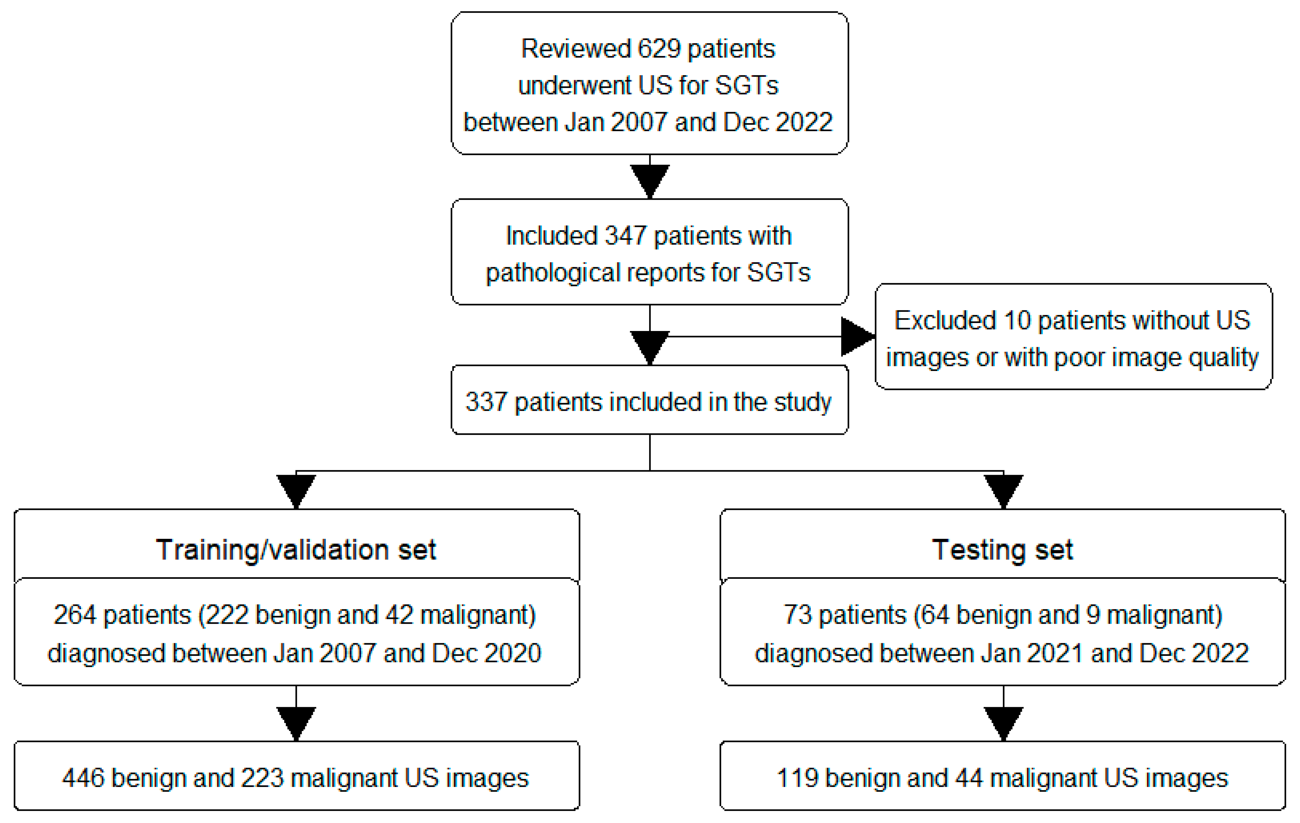
2.2. Inclusion Criteria
2.3. Data Collection
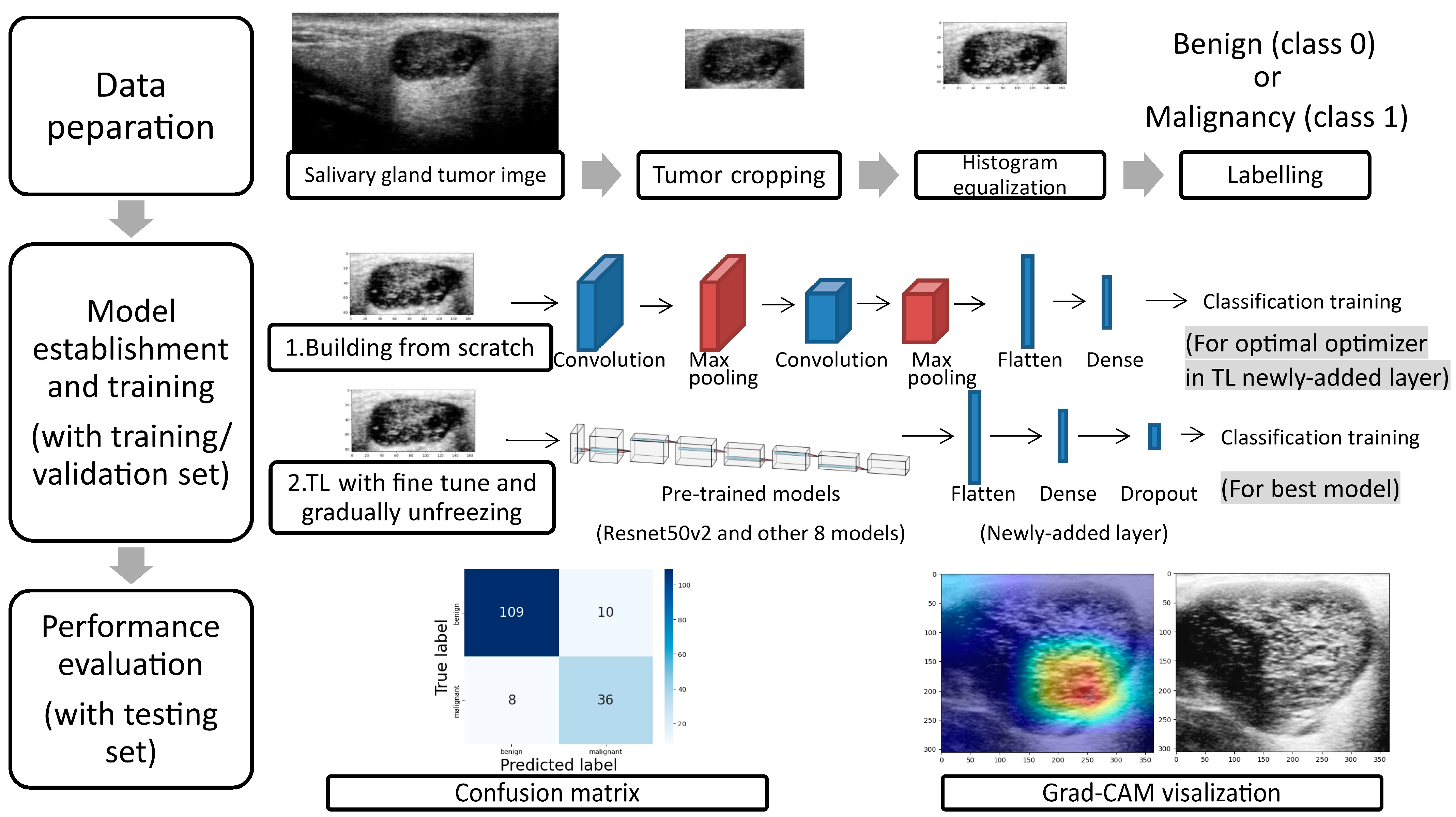
2.4. Data Preparation
2.5. Model Establishment
2.6. Statistical Analysis
3. Results
4. Discussion
5. Limitations
6. Conclusions
Supplementary Materials
Author Contributions
Funding
Institutional Review Board Statement
Informed Consent Statement
Data Availability Statement
Conflicts of Interest
References
- Guzzo, M.; Locati, L.D.; Prott, F.J.; Gatta, G.; McGurk, M.; Licitra, L. Major and minor salivary gland tumors. Crit. Rev. Oncol./Hematol. 2010, 74, 134–148. [Google Scholar] [CrossRef]
- Gontarz, M.; Bargiel, J.; Gąsiorowski, K.; Marecik, T.; Szczurowski, P.; Zapała, J.; Wyszyńska-Pawelec, G. Epidemiology of Primary Epithelial Salivary Gland Tumors in Southern Poland-A 26-Year, Clinicopathologic, Retrospective Analysis. J. Clin. Med. 2021, 10, 1663. [Google Scholar] [CrossRef]
- Żurek, M.; Rzepakowska, A.; Jasak, K.; Niemczyk, K. The Epidemiology of Salivary Glands Pathologies in Adult Population over 10 Years in Poland-Cohort Study. Int. J. Environ. Res. Public Health 2021, 19, 179. [Google Scholar] [CrossRef] [PubMed]
- Alsanie, I.; Rajab, S.; Cottom, H.; Adegun, O.; Agarwal, R.; Jay, A.; Graham, L.; James, J.; Barrett, A.W.; van Heerden, W.; et al. Distribution and Frequency of Salivary Gland Tumours: An International Multicenter Study. Head Neck Pathol. 2022, 16, 1043–1054. [Google Scholar] [CrossRef] [PubMed]
- Skálová, A.; Hyrcza, M.D.; Leivo, I. Update from the 5th Edition of the World Health Organization Classification of Head and Neck Tumors: Salivary Glands. Head Neck Pathol. 2022, 16, 40–53. [Google Scholar] [CrossRef]
- Peravali, R.K.; Bhat, H.H.; Upadya, V.H.; Agarwal, A.; Naag, S. Salivary gland tumors: A diagnostic dilemma! J. Maxillofac. Oral Surg. 2015, 14, 438–442. [Google Scholar] [CrossRef]
- Liu, Y.; Li, J.; Tan, Y.R.; Xiong, P.; Zhong, L.P. Accuracy of diagnosis of salivary gland tumors with the use of ultrasonography, computed tomography, and magnetic resonance imaging: A meta-analysis. Oral Surg. Oral Med. Oral Pathol. Oral Radiol. 2015, 119, 238–245.e232. [Google Scholar] [CrossRef]
- Sood, S.; McGurk, M.; Vaz, F. Management of Salivary Gland Tumours: United Kingdom National Multidisciplinary Guidelines. J. Laryngol. Otol. 2016, 130, S142–S149. [Google Scholar] [CrossRef] [PubMed]
- Thielker, J.; Grosheva, M.; Ihrler, S.; Wittig, A.; Guntinas-Lichius, O. Contemporary Management of Benign and Malignant Parotid Tumors. Front. Surg. 2018, 5, 39. [Google Scholar] [CrossRef]
- Lee, W.H.; Tseng, T.M.; Hsu, H.T.; Lee, F.P.; Hung, S.H.; Chen, P.Y. Salivary gland tumors: A 20-year review of clinical diagnostic accuracy at a single center. Oncol. Lett. 2014, 7, 583–587. [Google Scholar] [CrossRef]
- Lee, Y.Y.; Wong, K.T.; King, A.D.; Ahuja, A.T. Imaging of salivary gland tumours. Eur. J. Radiol. 2008, 66, 419–436. [Google Scholar] [CrossRef] [PubMed]
- Lo, W.C.; Chang, C.M.; Wang, C.T.; Cheng, P.W.; Liao, L.J. A Novel Sonographic Scoring Model in the Prediction of Major Salivary Gland Tumors. Laryngoscope 2020, 131, E157–E162. [Google Scholar] [CrossRef] [PubMed]
- Cheng, P.C.; Lo, W.C.; Chang, C.M.; Wen, M.H.; Cheng, P.W.; Liao, L.J. Comparisons among the Ultrasonography Prediction Model, Real-Time and Shear Wave Elastography in the Evaluation of Major Salivary Gland Tumors. Diagnostics 2022, 12, 2488. [Google Scholar] [CrossRef] [PubMed]
- Tama, B.A.; Kim, D.H.; Kim, G.; Kim, S.W.; Lee, S. Recent Advances in the Application of Artificial Intelligence in Otorhinolaryngology-Head and Neck Surgery. Clin. Exp. Otorhinolaryngol. 2020, 13, 326–339. [Google Scholar] [CrossRef] [PubMed]
- Yamashita, R.; Nishio, M.; Do, R.K.G.; Togashi, K. Convolutional neural networks: An overview and application in radiology. Insights Into Imaging 2018, 9, 611–629. [Google Scholar] [CrossRef]
- Alzubaidi, L.; Al-Amidie, M.; Al-Asadi, A.; Humaidi, A.J.; Al-Shamma, O.; Fadhel, M.A.; Zhang, J.; Santamaria, J.; Duan, Y. Novel Transfer Learning Approach for Medical Imaging with Limited Labeled Data. Cancers 2021, 13, 1590. [Google Scholar] [CrossRef]
- Hosna, A.; Merry, E.; Gyalmo, J.; Alom, Z.; Aung, Z.; Azim, M.A. Transfer learning: A friendly introduction. J. Big Data 2022, 9, 102. [Google Scholar] [CrossRef]
- Kim, H.E.; Cosa-Linan, A.; Santhanam, N.; Jannesari, M.; Maros, M.E.; Ganslandt, T. Transfer learning for medical image classification: A literature review. BMC Med. Imaging 2022, 22, 69. [Google Scholar] [CrossRef] [PubMed]
- Xie, Y.; Richmond, D. Pre-training on Grayscale ImageNet Improves Medical Image Classification. In Proceedings of the European Conference on Computer Vision (ECCV) Workshops, Munich, Germany, 8–14 September 2018; Part VI. pp. 476–484. [Google Scholar]
- Wang, Y.; Xie, W.; Huang, S.; Feng, M.; Ke, X.; Zhong, Z.; Tang, L. The Diagnostic Value of Ultrasound-Based Deep Learning in Differentiating Parotid Gland Tumors. J. Oncol. 2022, 2022, 8192999. [Google Scholar] [CrossRef]
- Gupta, N. A Pre-Trained Vs Fine-Tuning Methodology in Transfer Learning. J. Phys. Conf. Ser. 2021, 1947, 012028. [Google Scholar] [CrossRef]
- Tajbakhsh, N.; Shin, J.Y.; Gurudu, S.R.; Hurst, R.T.; Kendall, C.B.; Gotway, M.B.; Jianming, L. Convolutional Neural Networks for Medical Image Analysis: Full Training or Fine Tuning? IEEE Trans. Med. Imaging 2016, 35, 1299–1312. [Google Scholar] [CrossRef] [PubMed]
- Kumar, A.; Shen, R.; Bubeck, S.; Gunasekar, S. How to Fine-Tune Vision Models with SGD. arXiv 2022, arXiv:2211.09359. [Google Scholar]
- Howard, J.; Ruder, S. Universal language model fine-tuning for text classification. arXiv 2018, arXiv:1801.06146. [Google Scholar]
- Romero, M.; Interian, Y.; Solberg, T.; Valdes, G. Targeted transfer learning to improve performance in small medical physics datasets. Med. Phys. 2020, 47, 6246–6256. [Google Scholar] [CrossRef] [PubMed]
- Selvaraju, R.R.; Cogswell, M.; Das, A.; Vedantam, R.; Parikh, D.; Batra, D. Grad-CAM: Visual Explanations from Deep Networks via Gradient-Based Localization. In Proceedings of the 2017 IEEE International Conference on Computer Vision (ICCV), Venice, Italy, 22–29 October 2017; pp. 618–626. [Google Scholar]
- Căleanu, C.D.; Sîrbu, C.L.; Simion, G. Deep Neural Architectures for Contrast Enhanced Ultrasound (CEUS) Focal Liver Lesions Automated Diagnosis. Sensors 2021, 21, 4126. [Google Scholar] [CrossRef] [PubMed]
- Chou, T.-H.; Yeh, H.-J.; Chang, C.-C.; Tang, J.-H.; Kao, W.-Y.; Su, I.-C.; Li, C.-H.; Chang, W.-H.; Huang, C.-K.; Sufriyana, H.; et al. Deep learning for abdominal ultrasound: A computer-aided diagnostic system for the severity of fatty liver. J. Chin. Med. Assoc. 2021, 84, 842–850. [Google Scholar] [CrossRef]
- Zamanian, H.; Mostaar, A.; Azadeh, P.; Ahmadi, M. Implementation of Combinational Deep Learning Algorithm for Non-alcoholic Fatty Liver Classification in Ultrasound Images. J. Biomed. Phys. Eng. 2021, 11, 73–84. [Google Scholar] [CrossRef] [PubMed]
- Xiao, T.; Liu, L.; Li, K.; Qin, W.; Yu, S.; Li, Z. Comparison of Transferred Deep Neural Networks in Ultrasonic Breast Masses Discrimination. BioMed Res. Int. 2018, 2018, 4605191. [Google Scholar] [CrossRef]
- Kim, Y.-J.; Choi, Y.; Hur, S.-J.; Park, K.-S.; Kim, H.-J.; Seo, M.; Lee, M.K.; Jung, S.-L.; Jung, C.K. Deep convolutional neural network for classification of thyroid nodules on ultrasound: Comparison of the diagnostic performance with that of radiologists. Eur. J. Radiol. 2022, 152, 110335. [Google Scholar] [CrossRef]
- Guan, Q.; Wang, Y.; Du, J.; Qin, Y.; Lu, H.; Xiang, J.; Wang, F. Deep learning based classification of ultrasound images for thyroid nodules: A large scale of pilot study. Ann. Transl. Med. 2019, 7, 137. [Google Scholar] [CrossRef]
- Chi, J.; Walia, E.; Babyn, P.; Wang, J.; Groot, G.; Eramian, M. Thyroid Nodule Classification in Ultrasound Images by Fine-Tuning Deep Convolutional Neural Network. J. Digit. Imaging 2017, 30, 477–486. [Google Scholar] [CrossRef] [PubMed]
- Byra, M.; Galperin, M.; Ojeda-Fournier, H.; Olson, L.; O′Boyle, M.; Comstock, C.; Andre, M. Breast mass classification in sonography with transfer learning using a deep convolutional neural network and color conversion. Med. Phys. 2019, 46, 746–755. [Google Scholar] [CrossRef] [PubMed]
- Byra, M.; Styczynski, G.; Szmigielski, C.; Kalinowski, P.; Michałowski, Ł.; Paluszkiewicz, R.; Ziarkiewicz-Wróblewska, B.; Zieniewicz, K.; Sobieraj, P.; Nowicki, A. Transfer learning with deep convolutional neural network for liver steatosis assessment in ultrasound images. Int. J. Comput. Assist. Radiol. Surg. 2018, 13, 1895–1903. [Google Scholar] [CrossRef] [PubMed]
- Nie, Y.; Santis, L.D.; Carratù, M.; O’Nils, M.; Sommella, P.; Lundgren, J. Deep Melanoma classification with K-Fold Cross-Validation for Process optimization. In Proceedings of the 2020 IEEE International Symposium on Medical Measurements and Applications (MeMeA), Bari, Italy, 1 June–1 July 2020; pp. 1–6. [Google Scholar]
- Zhu, Y.C.; Jin, P.F.; Bao, J.; Jiang, Q.; Wang, X. Thyroid ultrasound image classification using a convolutional neural network. Ann. Transl. Med. 2021, 9, 1526. [Google Scholar] [CrossRef]


| Demographic Data (Mean (SD) or N (%)) | Training/Validation | Testing | p Value |
|---|---|---|---|
| N = 264 | N = 73 | ||
| Age, year | 53 (14) | 54 (15) | 0.493 |
| Sex | 0.453 | ||
| Female | 110 (42%) | 34 (47%) | |
| Male | 154 (58%) | 39 (53%) | |
| Side | 0.837 | ||
| Right | 141 (53%) | 38 (52%) | |
| Left | 123 (47%) | 35 (48%) | |
| Location | 0.302 | ||
| Parotid gland | 206 (78%) | 61 (84%) | |
| Submandibular gland | 58 (22%) | 12 (16%) | |
| Tumor size | |||
| Short axis, cm | 1.7 (0.6) | 1.6 (0.6) | 0.336 |
| Long axis, cm | 2.5 (1.0) | 2.4 (0.9) | 0.461 |
| Short–long-axis ratio | 0.7 (0.2) | 0.7 (0.1) | 0.586 |
| Pathological diagnoses | 0.450 | ||
| Benign tumors | 222 (84%) | 64 (88%) | |
| Malignant tumors | 42 (16%) | 9 (12%) |
| Pathological Reports | All | Training/Validation | Testing |
|---|---|---|---|
| N = 337 | N = 264 | N = 73 | |
| Benign salivary gland tumors | 286 | 222 | 64 |
| Pleomorphic adenoma | 114 (40%) | 91 (41%) | 23 (36%) |
| Warthin’s tumor | 106 (37%) | 83 (37%) | 23 (36%) |
| Other benign tumors (basal cell adenoma, oncocytoma, hemangioma, chronic sialadenitis, IgG4-associated sialadenitis, etc.) | 66 (23%) | 48 (22%) | 18 (28%) |
| Malignant salivary gland tumors | 51 | 42 | 9 |
| Poorly differentiated/undifferentiated carcinoma | 13 (26%) | 12 (29%) | 1 (11%) |
| Mucoepidermoid carcinoma | 12 (24%) | 7 (17%) | 5 (56%) |
| Metastatic carcinoma | 10 (20%) | 9 (22%) | 1 (11%) |
| Lymphoma | 5 (10%) | 5 (12%) | 0 (0%) |
| Lymphoepithelial carcinoma | 4 (8%) | 3 (7%) | 1 (11%) |
| Adenoid cystic carcinoma | 2 (4%) | 2 (5%) | 0 (0%) |
| Adenocarcinoma, | 2 (4%) | 1 (2%) | 1 (11%) |
| Acinic cell carcinoma | 1 (2%) | 1 (2%) | 0 (0%) |
| Carcinoma ex pleomorphic adenoma | 1 (2%) | 1 (2%) | 0 (0%) |
| Salivary duct carcinoma | 1 (2%) | 1 (2%) | 0 (0%) |
| Optimizer | SGD | RMSprop | Adagrad | Adadelta | Adam | Adamax | Nadam |
|---|---|---|---|---|---|---|---|
| ACC | 0.71 | 0.93 | 0.70 | 0.67 | 0.99 | 0.86 | 0.99 |
| LOSS | 0.56 | 0.21 | 0.59 | 0.62 | 0.04 | 0.33 | 0.05 |
| VAL_ACC | 0.61 | 0.62 | 0.67 | 0.67 | 0.68 * | 0.68 | 0.63 |
| VAL_LOSS | 0.70 | 1.01 | 0.67 | 0.63 | 1.54 | 0.69 | 1.49 |
| Layer | 2 | 3 | 4 | 5 | |||
| ACC | 0.99 | 0.97 | 0.79 | 0.63 | |||
| LOSS | 0.04 | 0.09 | 0.47 | 0.61 | |||
| VAL_ACC | 0.68 * | 0.60 | 0.72 | 0.67 | |||
| VAL_LOSS | 1.54 | 1.71 | 0.85 | 0.63 | |||
| Kernel size | 3 × 3 | 5 × 5 | 7 × 7 | ||||
| ACC | 0.99 | 0.98 | 0.97 | ||||
| LOSS | 0.04 | 0.07 | 0.07 | ||||
| VAL_ACC | 0.68 * | 0.63 | 0.51 | ||||
| VAL_LOSS | 1.54 | 1.86 | 1.89 | ||||
| Dropout | No | 10% | 30% | 50% | |||
| ACC | 0.99 | 0.92 | 0.83 | 0.78 | |||
| VAL_ACC | 0.68 * | 0.59 | 0.66 | 0.68 | |||
| Batch normalization | No | Yes | +dropout 10% | +dropout 50% | |||
| ACC | 0.99 | 0.90 | 0.81 | 0.73 | |||
| VAL_ACC | 0.68 * | 0.68 | 0.51 | 0.56 |
| Model | VGG16 | ResNet50V2 | MobileNetV2 | EfficientNetB0 | DenseNet121 | Xception | NASNetMobile | InceptionV3 | InceptionResNetV2 |
|---|---|---|---|---|---|---|---|---|---|
| AVG_ACC | 0.999 | 0.999 | 0.540 | 0.473 | 0.996 | 0.992 | 0.997 | 0.998 | 0.995 |
| AVG_LOSS | 0.030 | 0.007 | 0.924 | 0.924 | 0.020 | 0.032 | 0.018 | 0.019 | 0.033 |
| AVG_VAL_ACC | 0.789 * | 0.771 * | 0.505 | 0.693 | 0.798 * | 0.767 | 0.741 | 0.737 | 0.756 |
| AVG_VAL_LOSS | 0.633 | 1.348 | 0.694 | 0.441 | 0.720 | 1.022 | 0.981 | 0.996 | 0.967 |
| Model | DenseNet121 | VGG16 | ResNet50V2 |
|---|---|---|---|
| Unfreeze layer | conv4_block13_0_bn | Block4_conv1 | conv4_block5_preact_bn |
| Learning rate | 0.00001 | 0.0001 | 0.0001 |
| AVG_ACC | 1.000 | 0.732 | 0.996 |
| AVG_LOSS | 0.005 | 0.376 | 0.021 |
| AVG_VAL_ACC | 0.919 | 0.618 | 0.920 * |
| AVG_VAL_LOSS | 0.237 | 0.998 | 0.566 |
| TEST_ACC | 0.753 | 0.667 | 0.890 |
| TEST_LOSS | 0.543 | 0.692 | 0.527 |
| ResNet50V2 with Fine-Tuning and Gradual Unfreezing | Testing Set |
|---|---|
| Diagnostic result | |
| True positive | 36 |
| False negative | 8 |
| False positive | 10 |
| True negative | 109 |
| Diagnostic performance | |
| Accuracy | 89.0% |
| Sensitivity | 81.8% |
| Specificity | 91.6% |
| Positive predictive value, PPV | 78.3% |
| Negative predictive value, NPV | 93.2% |
Disclaimer/Publisher’s Note: The statements, opinions and data contained in all publications are solely those of the individual author(s) and contributor(s) and not of MDPI and/or the editor(s). MDPI and/or the editor(s) disclaim responsibility for any injury to people or property resulting from any ideas, methods, instructions or products referred to in the content. |
© 2023 by the authors. Licensee MDPI, Basel, Switzerland. This article is an open access article distributed under the terms and conditions of the Creative Commons Attribution (CC BY) license (https://creativecommons.org/licenses/by/4.0/).
Share and Cite
Cheng, P.-C.; Chiang, H.-H.K. Diagnosis of Salivary Gland Tumors Using Transfer Learning with Fine-Tuning and Gradual Unfreezing. Diagnostics 2023, 13, 3333. https://doi.org/10.3390/diagnostics13213333
Cheng P-C, Chiang H-HK. Diagnosis of Salivary Gland Tumors Using Transfer Learning with Fine-Tuning and Gradual Unfreezing. Diagnostics. 2023; 13(21):3333. https://doi.org/10.3390/diagnostics13213333
Chicago/Turabian StyleCheng, Ping-Chia, and Hui-Hua Kenny Chiang. 2023. "Diagnosis of Salivary Gland Tumors Using Transfer Learning with Fine-Tuning and Gradual Unfreezing" Diagnostics 13, no. 21: 3333. https://doi.org/10.3390/diagnostics13213333
APA StyleCheng, P.-C., & Chiang, H.-H. K. (2023). Diagnosis of Salivary Gland Tumors Using Transfer Learning with Fine-Tuning and Gradual Unfreezing. Diagnostics, 13(21), 3333. https://doi.org/10.3390/diagnostics13213333