
An Image-Based Prior Knowledge-Free Approach for a Multi-Material Decomposition in Photon-Counting Computed Tomography


Abstract
1. Introduction
2. Materials and Methods
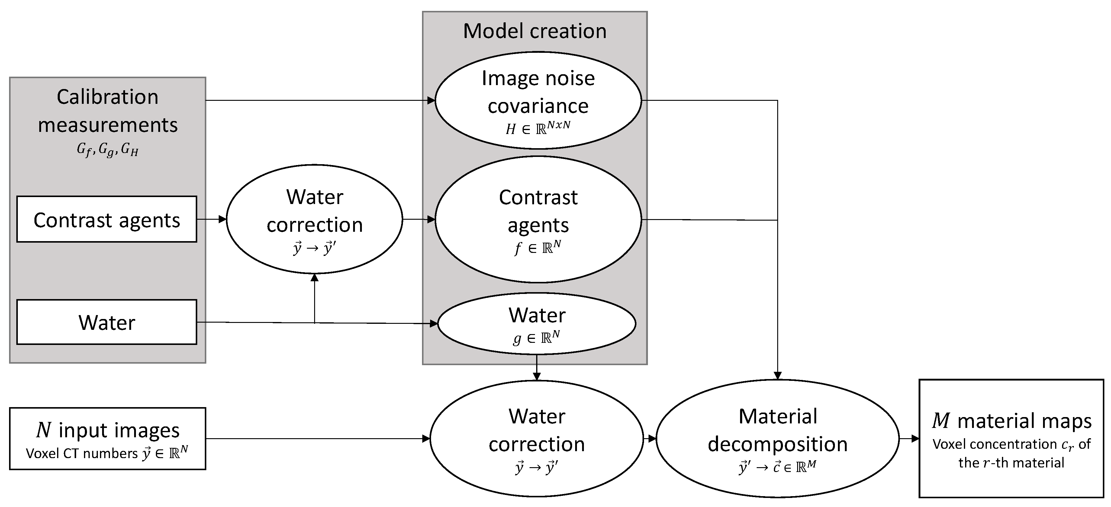
2.1. General Method
- is the vector of CT numbers of one image voxel at fixed row and column in the different spectral images;
- are the parameters on which the models depend;
- is the model of a CA CT number in one spectral image with coefficients to calibrate and a set of ground truth data ;
- is the model of the water CT number in one spectral image with coefficients to calibrate and a set of ground truth data ;
- is the model of the INCM with coefficients to calibrate and a set of ground truth data .
- Design matrix : If the -th BM () is a CA, is set to with the model of the -th BM CT number in the -th spectral image (), scaled to give the expected CT numbers at a concentration of 1 mg/mL for easy interpretation of the decomposition results. If the -th BM is water, is set to 1 for all p to ensure a linear water CE in the true water concentration for voxels containing at most water, interpreted as explained at the end of this section.
- Observation vector : For all () and the corresponding water model ,
- Covariance matrix : is set to .
- The user then estimates the material coefficients using the method of generalized LS. This means solving the linear system of equations
- The result is the best linear unbiased estimator for the overdetermined system
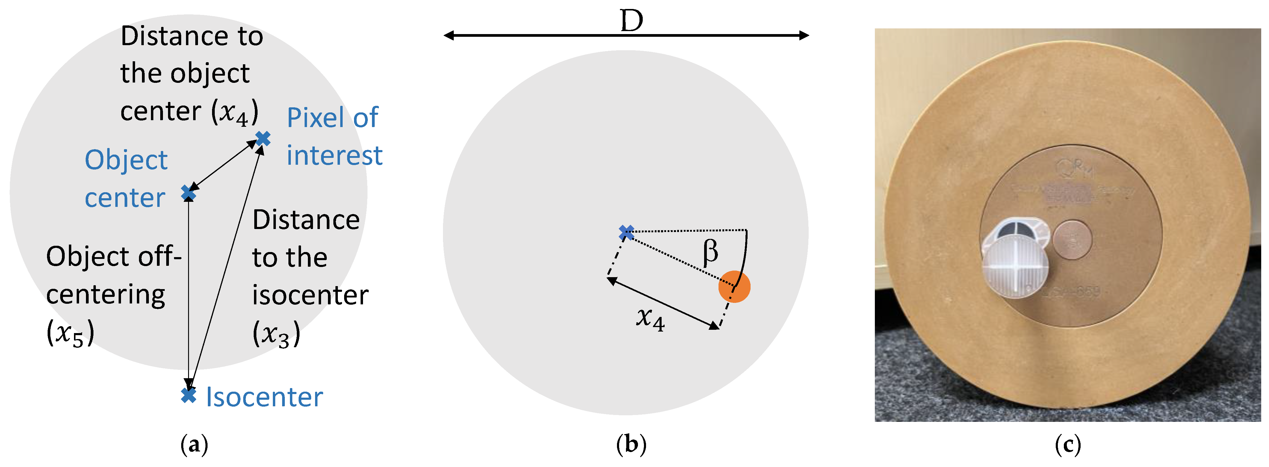
2.1.1. Model Parameters
- Object water-equivalent diameter (WED) [mm] ();
- X-ray tube current [mA] ();
- Voxel distance to the isocenter [mm] ();
- Voxel distance to the object center [mm] ();
- Object off-centering [mm] ().
2.1.2. Material Model Creation
2.1.3. Image Noise Covariance Model Creation
2.2. Experimental Setup and Image Acquisition
2.2.1. Material Description


| Parameter | Value | |||
|---|---|---|---|---|
| Water-Equivalent Phantom Diameter (mm) | 273 | 363 | ||
| Tube Current (mA) | 375 | 750 | 375 | 750 |
| Repetitions | 8 | 4 | 32 | 16 |
| Object Off-centering (mm) | 15, 45 | |||
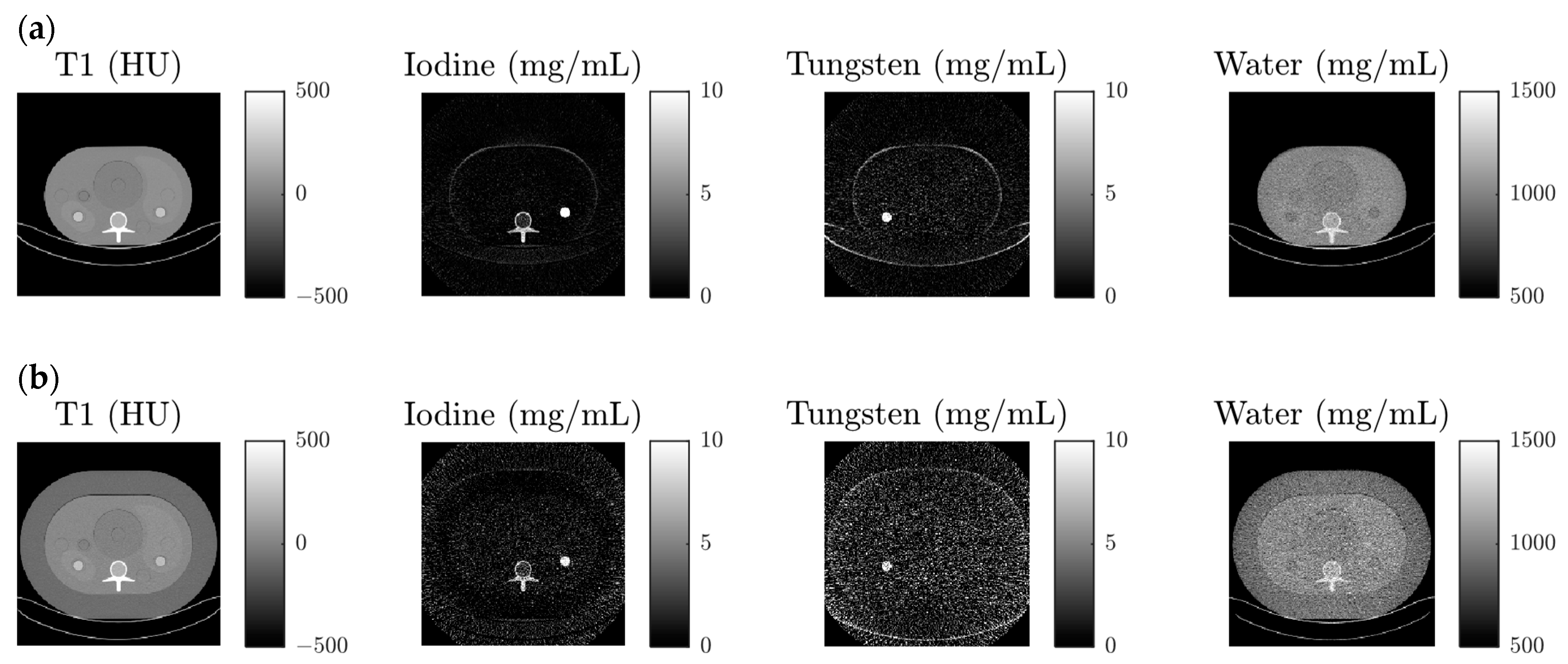
- Iodine dissolved in water (), hereafter called iodine;
- Tungsten dissolved in water (), hereafter called tungsten;
- Water ().
2.2.2. General Scan Setup
2.2.3. Calibration
2.2.4. Test Data Acquisition
2.3. Statistical Analysis
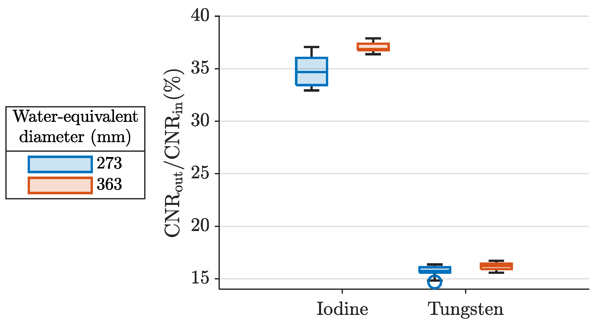
2.3.1. Contrast-to-Noise Ratio
- Iodine CE in the iodine insert;
- Tungsten CE in the tungsten insert.
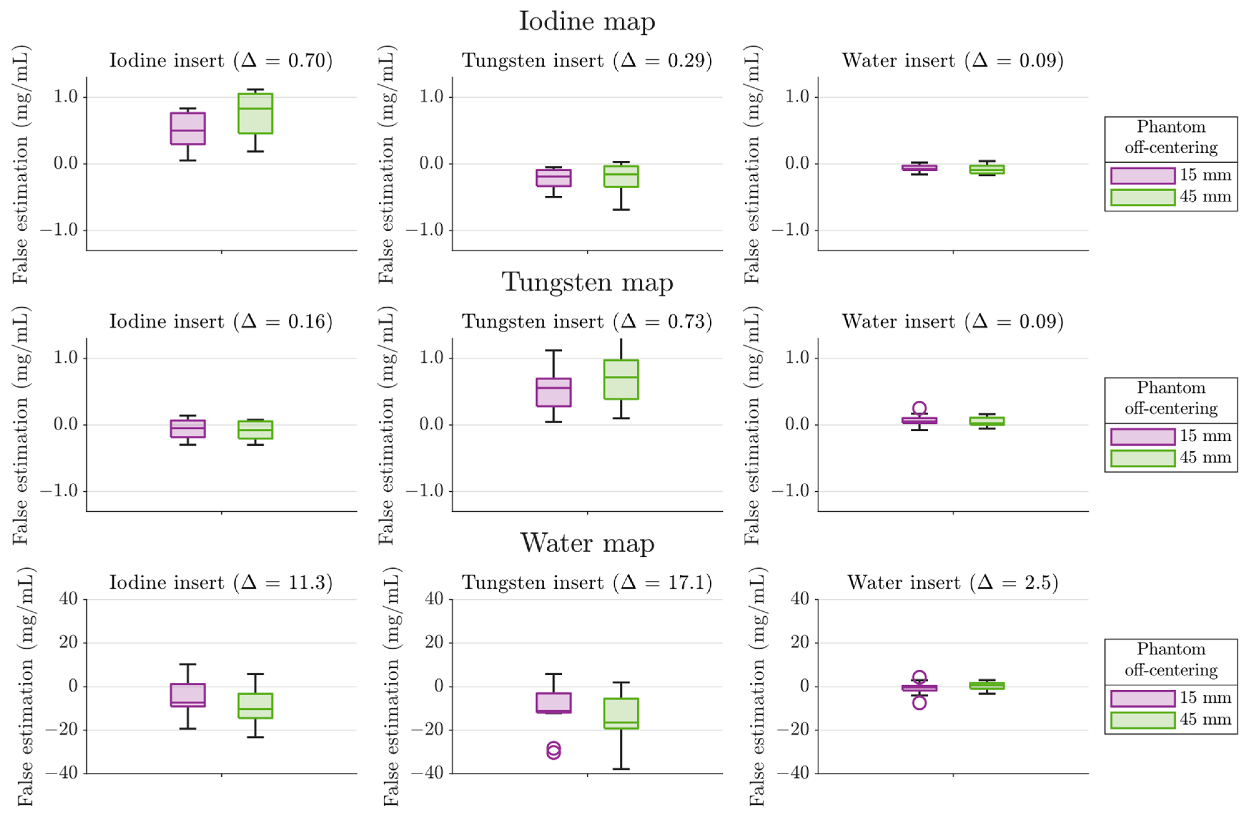
2.3.2. Estimation Accuracy
3. Results
3.1. Contrast-to-Noise Ratio
3.2. Estimation Accuracy
4. Discussion
4.1. Contrast-to-Noise Ratio
4.2. Estimation Accuracy
5. Conclusions
Author Contributions
Funding
Institutional Review Board Statement
Informed Consent Statement
Data Availability Statement
Acknowledgments
Conflicts of Interest
Appendix A
- For each scan and each ROI, we measured the INCM and averaged the matrices acquired in all reconstructed slices and all repetitions of equal setup. Assigning the ROI center coordinates and to each ROI, we created a look-up table for the INCM for each material and ROI in the parameters .
- We performed an iodine-tungsten-water-decomposition for each scan and ROI based on our material models once using the matching INCM from the look-up table and once using .
- We averaged the resulting material concentrations ROI-wise over all slices and scan repetitions. We then took the absolute differences between the resulting concentrations of the two decompositions. Those did not exceed 0.1 mg/mL in the CA maps and 2 mg/mL in the water map.
References
- Flohr, T.G.; McCollough, C.H.; Bruder, H.; Petersilka, M.; Gruber, K.; Süβ, C.; Grasruck, M.; Stierstorfer, K.; Krauss, B.; Raupach, R. First performance evaluation of a dual-source CT (DSCT) system. Eur. Radiol. 2006, 16, 256–268. [Google Scholar] [CrossRef] [PubMed]
- Goshen, L.; Sosna, J.; Carmi, R.; Kafri, G.; Iancu, I.; Altman, A. An iodine-calcium separation analysis and virtually non-contrasted image generation obtained with single source dual energy MDCT. In Proceedings of the 2008 IEEE Nuclear Science Symposium Conference Record, Dresden, Germany, 19–25 October 2008; pp. 3868–3870. [Google Scholar]
- Heismann, B.J.; Wirth, S.; Janssen, S.; Spreiter, Q. Technology and image results of a spectral CT system. In Proceedings of the Medical Imaging 2004: Physics of Medical Imaging, San Diego, CA, USA, 14–19 February 2004; pp. 52–59. [Google Scholar]
- Schwarz, F.; Ruzsics, B.; Schoepf, U.J.; Bastarrika, G.; Chiaramida, S.A.; Abro, J.A.; Brothers, R.L.; Vogt, S.; Schmidt, B.; Costello, P. Dual-energy CT of the heart—Principles and protocols. Eur. J. Radiol. 2008, 68, 423–433. [Google Scholar] [CrossRef] [PubMed]
- Badea, C.T.; Johnston, S.; Johnson, B.; Lin, M.; Hedlund, L.; Johnson, G.A. A dual micro-CT system for small animal imaging. In Proceedings of the Medical imaging 2008: Physics of Medical Imaging, San Diego, CA, USA, 16–21 February 2008; pp. 1294–1303. [Google Scholar]
- Kalender, W.A.; Buchenau, S.; Deak, P.; Kellermeier, M.; Langner, O.; van Straten, M.; Vollmar, S.; Wilharm, S. Technical approaches to the optimisation of CT. Phys. Medica 2008, 24, 71–79. [Google Scholar] [CrossRef] [PubMed]
- Sahni, V.; Shinagare, A.; Silverman, S. Virtual unenhanced CT images acquired from dual-energy CT urography: Accuracy of attenuation values and variation with contrast material phase. Clin. Radiol. 2013, 68, 264–271. [Google Scholar] [CrossRef] [PubMed]
- Kang, D.K.; Schoepf, U.J.; Bastarrika, G.; Nance, J.W., Jr.; Abro, J.A.; Ruzsics, B. Dual-energy computed tomography for integrative imaging of coronary artery disease: Principles and clinical applications. Semin. Ultrasound CT MRI 2010, 31, 276–291. [Google Scholar] [CrossRef] [PubMed]
- Johnson, T.R.; Krauss, B.; Sedlmair, M.; Grasruck, M.; Bruder, H.; Morhard, D.; Fink, C.; Weckbach, S.; Lenhard, M.; Schmidt, B. Material differentiation by dual energy CT: Initial experience. Eur. Radiol. 2007, 17, 1510–1517. [Google Scholar] [CrossRef] [PubMed]
- Laugerette, A.; Schwaiger, B.J.; Brown, K.; Frerking, L.C.; Kopp, F.K.; Mei, K.; Sellerer, T.; Kirschke, J.; Baum, T.; Gersing, A.S. DXA-equivalent quantification of bone mineral density using dual-layer spectral CT scout scans. Eur. Radiol. 2019, 29, 4624–4634. [Google Scholar] [CrossRef]
- Mory, C.; Sixou, B.; Si-Mohamed, S.; Boussel, L.; Rit, S. Comparison of five one-step reconstruction algorithms for spectral CT. Phys. Med. Biol. 2018, 63, 235001. [Google Scholar] [CrossRef]
- Möhler, C.; Wohlfahrt, P.; Richter, C.; Greilich, S. Range prediction for tissue mixtures based on dual-energy CT. Phys. Med. Biol. 2016, 61, N268. [Google Scholar] [CrossRef]
- Maaß, C.; Baer, M.; Kachelrieß, M. Image-based dual energy CT using optimized precorrection functions: A practical new approach of material decomposition in image domain. Med. Phys. 2009, 36, 3818–3829. [Google Scholar] [CrossRef]
- Yu, L.; Christner, J.A.; Leng, S.; Wang, J.; Fletcher, J.G.; McCollough, C.H. Virtual monochromatic imaging in dual-source dual-energy CT: Radiation dose and image quality. Med. Phys. 2011, 38, 6371–6379. [Google Scholar] [CrossRef] [PubMed]
- Schmidt, B.; Flohr, T. Principles and applications of dual source CT. Phys. Medica 2020, 79, 36–46. [Google Scholar] [CrossRef] [PubMed]
- Flohr, T.; Petersilka, M.; Henning, A.; Ulzheimer, S.; Ferda, J.; Schmidt, B. Photon-counting CT review. Phys. Medica 2020, 79, 126–136. [Google Scholar] [CrossRef] [PubMed]
- U.S. Food and Drug Administration. FDA Clears First Major Imaging Device Advancement for Computed Tomography in Nearly a Decade. Available online: https://www.fda.gov/news-events/press-announcements/fda-clears-first-major-imaging-device-advancement-computed-tomography-nearly-decade (accessed on 24 July 2023).
- Allmendinger, T.; Nowak, T.; Flohr, T.; Klotz, E.; Hagenauer, J.; Alkadhi, H.; Schmidt, B. Photon-counting detector CT-based vascular calcium removal algorithm: Assessment using a cardiac motion phantom. Investig. Radiol. 2022, 57, 399. [Google Scholar] [CrossRef] [PubMed]
- Rajendran, K.; Petersilka, M.; Henning, A.; Shanblatt, E.R.; Schmidt, B.; Flohr, T.G.; Ferrero, A.; Baffour, F.; Diehn, F.E.; Yu, L. First clinical photon-counting detector CT system: Technical evaluation. Radiology 2022, 303, 130–138. [Google Scholar] [CrossRef] [PubMed]
- Jost, G.; McDermott, M.; Gutjahr, R.; Nowak, T.; Schmidt, B.; Pietsch, H. New contrast media for K-edge imaging with photon-counting detector CT. Investig. Radiol. 2023, 58, 515–522. [Google Scholar] [CrossRef] [PubMed]
- Schöckel, L.; Jost, G.; Seidensticker, P.; Lengsfeld, P.; Palkowitsch, P.; Pietsch, H. Developments in X-ray contrast media and the potential impact on computed tomography. Investig. Radiol. 2020, 55, 592–597. [Google Scholar] [CrossRef]
- Sartoretti, T.; McDermott, M.C.; Stammen, L.; Martens, B.; Moser, L.J.; Jost, G.; Pietsch, H.; Gutjahr, R.; Nowak, T.; Schmidt, B. Tungsten-Based Contrast Agent for Photon-Counting Detector CT Angiography in Calcified Coronaries: Comparison to Iodine in a Cardiovascular Phantom. Investig. Radiol. 2023. [Google Scholar] [CrossRef]
- Ren, L.; McCollough, C.; Yu, L. Three-Material Decomposition in Multi-energy CT: Impact of Prior Information on Noise and Bias. In Proceedings of the Medical Imaging 2018: Physics of Medical Imaging, Houston, TX, USA, 10–15 February 2018; Volume 10573. [Google Scholar] [CrossRef]
- Clark, D.P.; Badea, C.T. Spectral diffusion: An algorithm for robust material decomposition of spectral CT data. Phys. Med. Biol. 2014, 59, 6445. [Google Scholar] [CrossRef]
- Fredette, N.R.; Kavuri, A.; Das, M. Multi-step material decomposition for spectral computed tomography. Phys. Med. Biol. 2019, 64, 145001. [Google Scholar] [CrossRef] [PubMed]
- Mendonça, P.R.; Bhotika, R.; Maddah, M.; Thomsen, B.; Dutta, S.; Licato, P.E.; Joshi, M.C. Multi-material decomposition of spectral CT images. In Proceedings of the Medical Imaging 2010: Physics of Medical Imaging, San Diego, TX, USA, 13–18 February 2010; pp. 633–641. [Google Scholar]
- Long, Y.; Fessler, J.A. Multi-material decomposition using statistical image reconstruction for spectral CT. IEEE Trans. Med. Imaging 2014, 33, 1614–1626. [Google Scholar] [CrossRef]
- Baturin, P.; Alivov, Y.; Molloi, S. Spectral CT imaging of vulnerable plaque with two independent biomarkers. Phys. Med. Biol. 2012, 57, 4117. [Google Scholar] [CrossRef] [PubMed]
- Liu, X.; Yu, L.; Primak, A.N.; McCollough, C.H. Quantitative imaging of element composition and mass fraction using dual-energy CT: Three-material decomposition. Med. Phys. 2009, 36, 1602–1609. [Google Scholar] [CrossRef] [PubMed]
- Tang, X.; Ren, Y. On the conditioning of basis materials and its impact on multimaterial decomposition-based spectral imaging in photon-counting CT. Med. Phys. 2021, 48, 1100–1116. [Google Scholar] [CrossRef] [PubMed]
- Curtis, T.E.; Roeder, R.K. Effects of calibration methods on quantitative material decomposition in photon-counting spectral computed tomography using a maximum a posteriori estimator. Med. Phys. 2017, 44, 5187–5197. [Google Scholar] [CrossRef] [PubMed]
- Zhao, W.; Vernekohl, D.; Han, F.; Han, B.; Peng, H.; Yang, Y.; Xing, L.; Min, J.K. A unified material decomposition framework for quantitative dual-and triple-energy CT imaging. Med. Phys. 2018, 45, 2964–2977. [Google Scholar] [CrossRef] [PubMed]
- Liu, S.Z.; Tivnan, M.; Osgood, G.M.; Siewerdsen, J.H.; Stayman, J.W.; Zbijewski, W. Model-based three-material decomposition in dual-energy CT using the volume conservation constraint. Phys. Med. Biol. 2022, 67, 145006. [Google Scholar] [CrossRef] [PubMed]
- Buzug, T.M. Computed Tomography; Springer: Berlin/Heidelberg, Germany, 2011. [Google Scholar]
- Lee, S.; Choi, Y.-N.; Kim, H.-J. Quantitative material decomposition using spectral computed tomography with an energy-resolved photon-counting detector. Phys. Med. Biol. 2014, 59, 5457. [Google Scholar] [CrossRef] [PubMed]
- Malusek, A.; Karlsson, M.; Magnusson, M.; Carlsson, G.A. The potential of dual-energy computed tomography for quantitative decomposition of soft tissues to water, protein and lipid in brachytherapy. Phys. Med. Biol. 2013, 58, 771. [Google Scholar] [CrossRef]
- McCollough, C.; Bakalyar, D.M.; Bostani, M.; Brady, S.; Boedeker, K.; Boone, J.M.; Chen-Mayer, H.H.; Christianson, O.I.; Leng, S.; Li, B. Use of water equivalent diameter for calculating patient size and size-specific dose estimates (SSDE) in CT: The report of AAPM task group 220. AAPM Rep. 2014, 2014, 6. [Google Scholar]
- Brooks, R.A. A quantitative theory of the Hounsfield unit and its application to dual energy scanning. J. Comput. Assist. Tomogr. 1977, 1, 487–493. [Google Scholar] [CrossRef] [PubMed]
- Krauss, B.; Schmidt, B.; Flohr, T. Dual Energy CT in Clinical Practice Medical Radiology; Springer: Heidelberg, Germany, 2011. [Google Scholar]
- Kalender, W.A. Computed Tomography: Fundamentals, System Technology, Image Quality, Applications; John Wiley & Sons: Hoboken, NJ, USA, 2011. [Google Scholar]
- Mihl, C.; Kok, M.; Wildberger, J.E.; Altintas, S.; Labus, D.; Nijssen, E.C.; Hendriks, B.M.; Kietselaer, B.L.; Das, M. Coronary CT angiography using low concentrated contrast media injected with high flow rates: Feasible in clinical practice. Eur. J. Radiol. 2015, 84, 2155–2160. [Google Scholar] [CrossRef] [PubMed]
- Huang, R.Y.; Chai, B.B.; Lee, T.C. Effect of region-of-interest placement in bolus tracking cerebral computed tomography angiography. Neuroradiology 2013, 55, 1183–1188. [Google Scholar] [CrossRef] [PubMed]
- Ichikawa, T.; Erturk, S.M.; Araki, T. Multiphasic contrast-enhanced multidetector-row CT of liver: Contrast-enhancement theory and practical scan protocol with a combination of fixed injection duration and patients’ body-weight-tailored dose of contrast material. Eur. J. Radiol. 2006, 58, 165–176. [Google Scholar] [CrossRef] [PubMed]
- National Institute of Standards and Technology. X-ray Transition Energies Database. Available online: https://physics.nist.gov/PhysRefData/XrayTrans/Html/search.html (accessed on 24 July 2023).
- Stierstorfer, K.; Rauscher, A.; Boese, J.; Bruder, H.; Schaller, S.; Flohr, T. Weighted FBP—A simple approximate 3D FBP algorithm for multislice spiral CT with good dose usage for arbitrary pitch. Phys. Med. Biol. 2004, 49, 2209. [Google Scholar] [CrossRef] [PubMed]
- Boone, J.M.; Brink, J.A.; Edyvean, S.; Huda, W.; Leitz, W.; McCollough, C.; McNitt-Gray, M.; Dawson, P.; Deluca, P.; Seltzer, S. Radiation dose and image-quality assessment in computed tomography. J. ICRU 2012, 12, 9–149. [Google Scholar]
- Barlow, R.J. Statistics: A Guide to the Use of Statistical Methods in the Physical Sciences; John Wiley & Sons: Hoboken, NJ, USA, 1993; Volume 29. [Google Scholar]
- Mergen, V.; Eberhard, M.; Manka, R.; Euler, A.; Alkadhi, H. First in-human quantitative plaque characterization with ultra-high resolution coronary photon-counting CT angiography. Front. Cardiovasc. Med. 2022, 9, 981012. [Google Scholar] [CrossRef]
- Si-Mohamed, S.A.; Boccalini, S.; Lacombe, H.; Diaw, A.; Varasteh, M.; Rodesch, P.-A.; Dessouky, R.; Villien, M.; Tatard-Leitman, V.; Bochaton, T. Coronary CT angiography with photon-counting CT: First-in-human results. Radiology 2022, 303, 303–313. [Google Scholar] [CrossRef]
- Sartoretti, T.; Landsmann, A.; Nakhostin, D.; Eberhard, M.; Roeren, C.; Mergen, V.; Higashigaito, K.; Raupach, R.; Alkadhi, H.; Euler, A. Quantum iterative reconstruction for abdominal photon-counting detector CT improves image quality. Radiology 2022, 303, 339–348. [Google Scholar] [CrossRef]
| Parameter | Value |
|---|---|
| Tube Voltage (kV) | 140 (Tube A only) |
| Threshold Energies (keV) | 20, 55, 72, 90 |
| Scan Mode | Spiral |
| Rotation Time (s) | 0.25 |
| Pitch | 0.55 |
| Axial Collimation (mm) | 96 × 0.4 |
| Reconstruction Algorithm | Weighted Filtered Backprojection |
| Kernel | Qr40 |
| Field of View (mm) | 500 |
| Matrix Size | 512 × 512 |
| Slice Thickness (mm) | 2.0 |
| Slice Increment (mm) | 2.0 |
| Parameter | Value | ||||
|---|---|---|---|---|---|
| Phantom Diameter (mm) | 150 | 200 | 250 | 300 | 350 |
| Tube Current (mA) | 60, 80, 100, 120, 140 | 110, 140, 180, 210, 250 | 170, 220, 280, 330, 390 | 240, 320, 400, 480, 560 | 330, 440, 540, 650, 760 |
| Object Off-centering (mm) | 0, 30, 60 | ||||
| Insert Distance to the Object Center (mm) | 30 | ||||
| Resulting Insert Distances to the Isocenter (mm) | 0, 42, 67 | ||||
Disclaimer/Publisher’s Note: The statements, opinions and data contained in all publications are solely those of the individual author(s) and contributor(s) and not of MDPI and/or the editor(s). MDPI and/or the editor(s) disclaim responsibility for any injury to people or property resulting from any ideas, methods, instructions or products referred to in the content. |
© 2024 by the authors. Licensee MDPI, Basel, Switzerland. This article is an open access article distributed under the terms and conditions of the Creative Commons Attribution (CC BY) license (https://creativecommons.org/licenses/by/4.0/).
Share and Cite
Neumann, J.; Nowak, T.; Schmidt, B.; von Zanthier, J. An Image-Based Prior Knowledge-Free Approach for a Multi-Material Decomposition in Photon-Counting Computed Tomography. Diagnostics 2024, 14, 1262. https://doi.org/10.3390/diagnostics14121262
Neumann J, Nowak T, Schmidt B, von Zanthier J. An Image-Based Prior Knowledge-Free Approach for a Multi-Material Decomposition in Photon-Counting Computed Tomography. Diagnostics. 2024; 14(12):1262. https://doi.org/10.3390/diagnostics14121262
Chicago/Turabian StyleNeumann, Jonas, Tristan Nowak, Bernhard Schmidt, and Joachim von Zanthier. 2024. "An Image-Based Prior Knowledge-Free Approach for a Multi-Material Decomposition in Photon-Counting Computed Tomography" Diagnostics 14, no. 12: 1262. https://doi.org/10.3390/diagnostics14121262
APA StyleNeumann, J., Nowak, T., Schmidt, B., & von Zanthier, J. (2024). An Image-Based Prior Knowledge-Free Approach for a Multi-Material Decomposition in Photon-Counting Computed Tomography. Diagnostics, 14(12), 1262. https://doi.org/10.3390/diagnostics14121262