
Applicability of the CT Radiomics of Skeletal Muscle and Machine Learning for the Detection of Sarcopenia and Prognostic Assessment of Disease Progression in Patients with Gastric and Esophageal Tumors

 , , , , and
Abstract
1. Introduction
1.1. Gastric and Esophageal Tumors
1.2. Radiomics
1.3. Purpose of the Study
- (1)
- Sarcopenia detected with routine CT scans influences disease progression in patients with gastroesophageal cancer.
- (2)
- The CT radiomics of skeletal muscle and machine learning can detect sarcopenia and predict tumor progression.
2. Material and Methods
2.1. Muscle Segmentation and Assessment of Sarcopenia
2.2. Statistics
2.3. Radiomics Model and Machine Learning
3. Results
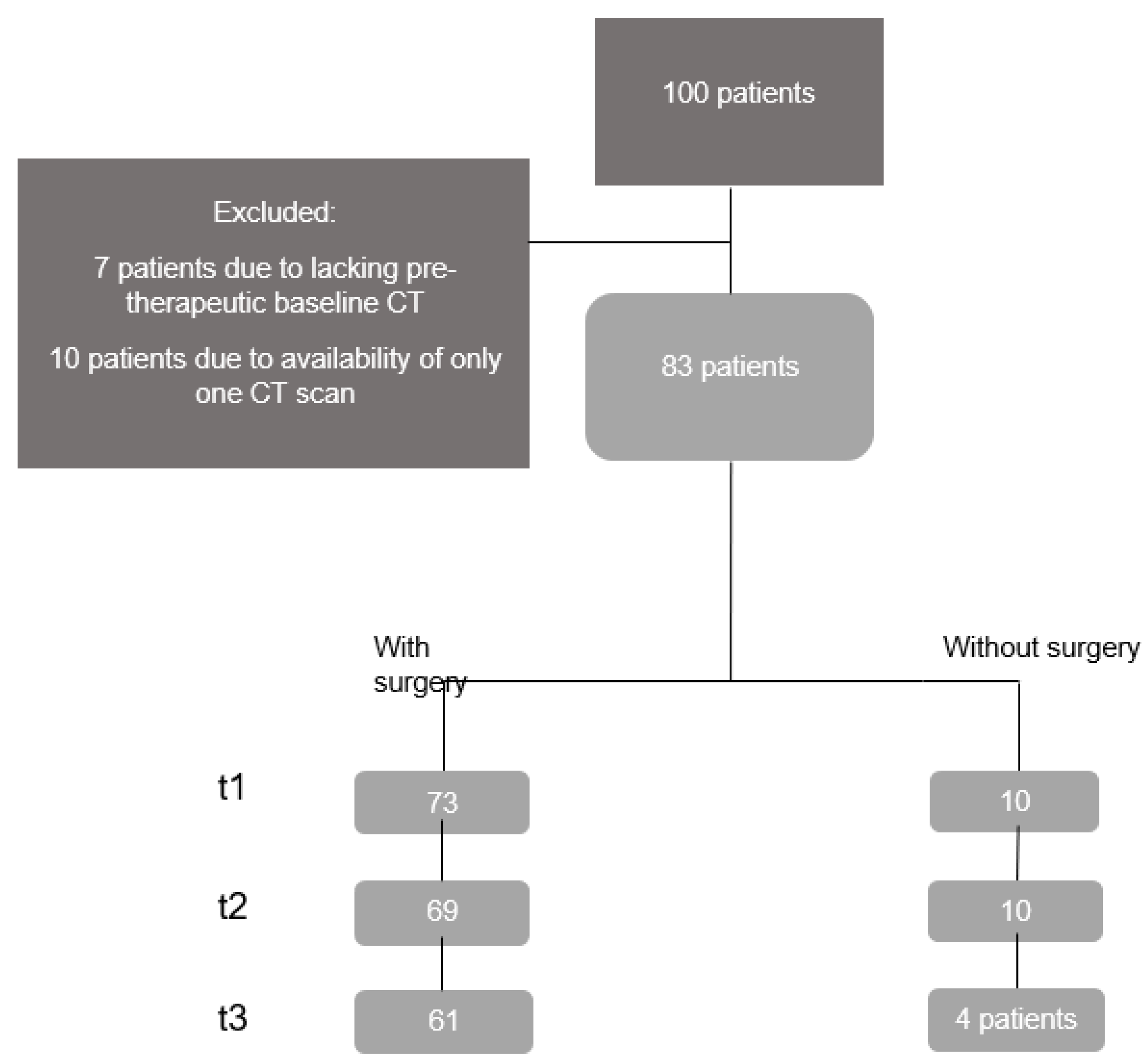
3.1. Patients’ Demographic and Clinical Data
3.2. Sarcopenia
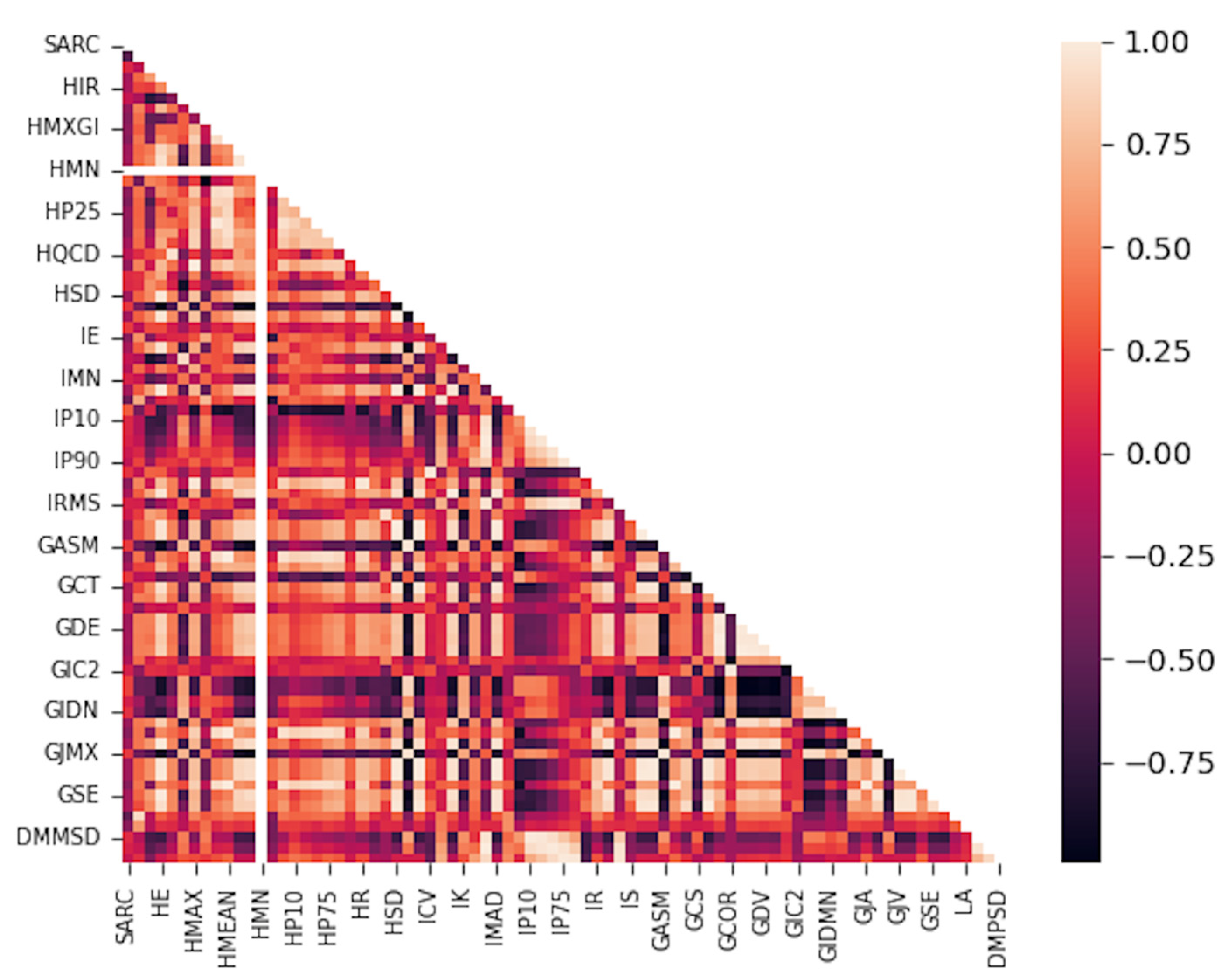
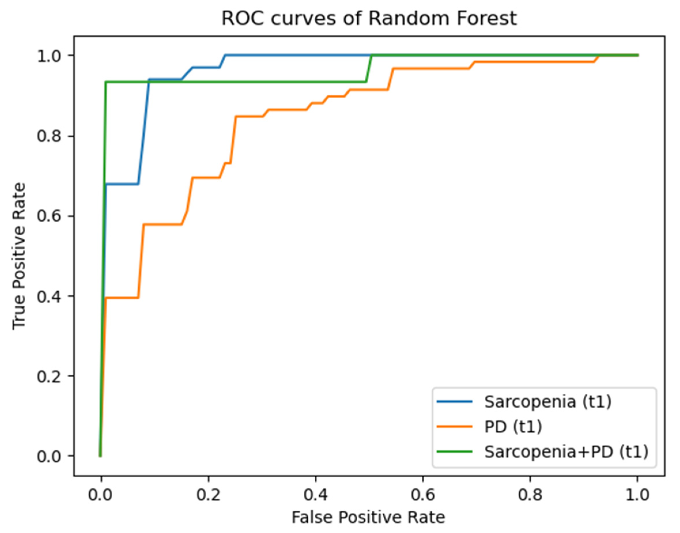
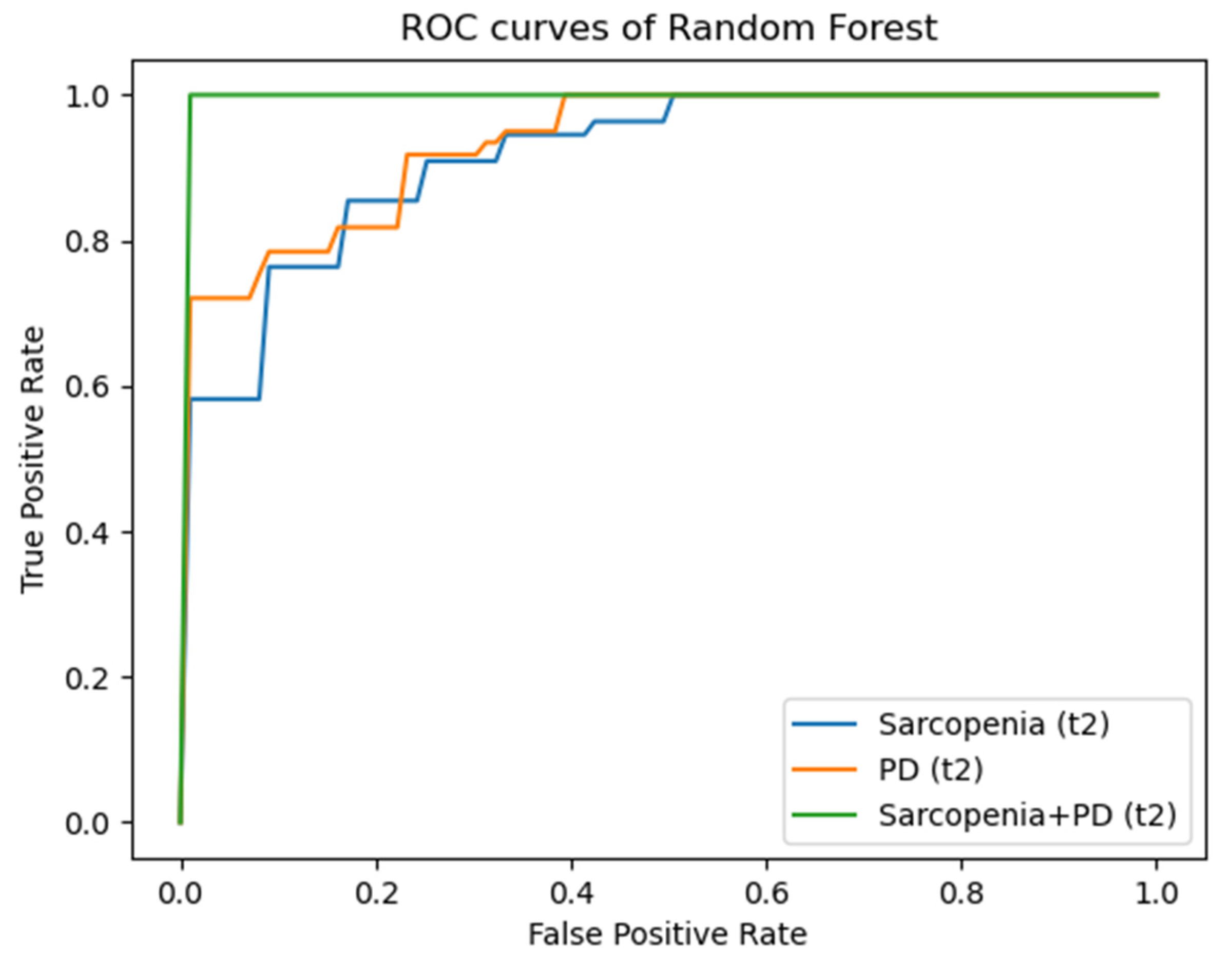
3.3. Radiomics
4. Discussion
4.1. Assessment of Sarcopenia
4.2. Effect of Sarcopenia
4.3. Radiomics
4.4. Limitations
5. Conclusions
Author Contributions
Funding
Institutional Review Board Statement
Informed Consent Statement
Data Availability Statement
Conflicts of Interest
Appendix A

| Radiomics Features of First Order | Radiomics Features of Second Order: Gray Level Co-Occurrence Matrix (GLCM) |
|---|---|
| Histogram Minimum | Joint Maximum |
| Histogram Maximum | Joint Average |
| Histogram Range | Standard Deviation |
| Histogram Mean | Joint Variance |
| Histogram Variance | Joint Entropy |
| Histogram Standard Deviation | Difference Average |
| Histogram Skewness | Difference Variance |
| Histogram Kurtosis | Difference Entropy |
| Histogram Entropy | Sum of Averages |
| Histogram Uniformity | Sum of Variance |
| Histogram Mean Absolute Deviation | Sum of Entropy |
| Histogram Robust Mean Absolute Deviation | Angular Second Moment |
| Histogram Median Absolute Deviation | Contrast |
| Histogram Coefficient Variation | Dissimilarity |
| Histogram Quartile Coefficient Dispersion | Inverse Difference |
| Histogram Interquartile Range | Inverse Difference Normalized |
| Histogram P10th | Inverse Difference Moment |
| Histogram P25th | Inverse Difference Moment Normalized |
| Histogram P50th | Joint Maximum |
| Histogram P75th | Joint Average |
| Histogram P90th | Standard Deviation |
| Histogram Minimum Histogram Gradient Intensity | Joint Variance |
| Histogram Maximum Histogram Gradient Intensity | Joint Entropy |
| Intensity Minimum | Difference Average |
| Intensity Maximum | Difference Variance |
| Intensity Range | Difference Entropy |
| Intensity Mean | Sum of Averages |
| Intensity Variance | Sum of Variance |
| Intensity Standard Deviation | Sum of Entropy |
| Intensity Skewness | Angular Second Moment |
| Intensity Kurtosis | Contrast |
| Intensity Energy | Dissimilarity |
| Intensity P10th | Inverse Variance |
| Intensity P25th | Correlation |
| Intensity P50th | Auto Correlation |
| Intensity P75th | Cluster Shade |
| Intensity P90th | Cluster Prominence |
| Intensity Root Mean Square | Cluster Tendency |
| Intensity Mean Absolute Deviation | Information Correlation 1 |
| Intensity Robust Mean Absolute Deviation | Information Correlation 2 |
| Intensity Median Absolute Deviation | Inverse Variance 41 |
| Intensity Coefficient Variation | |
| Intensity Quartile Coefficient Dispersion | |
| Intensity Interquartile Range 44 |
References
- Muscaritoli, M.; Anker, S.D.; Argilés, J.; Aversa, Z.; Bauer, J.M.; Biolo, G.; Boirie, Y.; Bosaeus, I.; Cederholm, T.; Costelli, P.; et al. Consensus definition of sarcopenia, cachexia and pre-cachexia: Joint document elaborated by Special Interest Groups (SIG) “cachexia-anorexia in chronic wasting diseases” and “nutrition in geriatrics”. Clin. Nutr. 2010, 29, 154–159. [Google Scholar] [CrossRef]
- Meza-Valderrama, D.; Marco, E.; Dávalos-Yerovi, V.; Muns, M.D.; Tejero-Sánchez, M.; Duarte, E.; Sánchez-Rodríguez, D. Sarcopenia, Malnutrition, and Cachexia: Adapting Definitions and Terminology of Nutritional Disorders in Older People with Cancer. Nutrients 2021, 13, 761. [Google Scholar] [CrossRef] [PubMed]
- Rezende, I.F.B.; Conceição-Machado, M.E.P.; Souza, V.S.; Santos, E.M.D.; Silva, L.R. Sarcopenia in children and adolescents with chronic liver disease. J. Pediatr. 2020, 96, 439–446. [Google Scholar] [CrossRef] [PubMed]
- Ritz, A.; Kolorz, J.; Hubertus, J.; Ley-Zaporozhan, J.; von Schweinitz, D.; Koletzko, S.; Häberle, B.; Schmid, I.; Kappler, R.; Berger, M.; et al. Sarcopenia is a prognostic outcome marker in children with high-risk hepatoblastoma. Pediatr. Blood Cancer 2021, 68, e28862. [Google Scholar] [CrossRef] [PubMed]
- Triarico, S.; Rinninella, E.; Mele, M.C.; Cintoni, M.; Attinà, G.; Ruggiero, A. Prognostic impact of sarcopenia in children with cancer: A focus on the psoas muscle area (PMA) imaging in the clinical practice. Eur. J. Clin. Nutr. 2022, 76, 783–788. [Google Scholar] [CrossRef]
- Berger, M.J.; Doherty, T.J. Sarcopenia: Prevalence, mechanisms, and functional consequences. Interdiscip. Top. Gerontol. 2010, 37, 94–114. [Google Scholar] [CrossRef]
- Simonsen, C.; Kristensen, T.S.; Sundberg, A.; Wielsøe, S.; Christensen, J.; Hansen, C.P.; Burgdorf, S.K.; Suetta, C.; de Heer, P.; Svendsen, L.B.; et al. Assessment of sarcopenia in patients with upper gastrointestinal tumors: Prevalence and agreement between computed tomography and dual-energy x-ray absorptiometry. Clin. Nutr. 2021, 40, 2809–2816. [Google Scholar] [CrossRef]
- Martin, L.; Birdsell, L.; Macdonald, N.; Reiman, T.; Clandinin, M.T.; McCargar, L.J.; Murphy, R.; Ghosh, S.; Sawyer, M.B.; Baracos, V.E. Cancer cachexia in the age of obesity: Skeletal muscle depletion is a powerful prognostic factor, independent of body mass index. J. Clin. Oncol. 2013, 31, 1539–1547. [Google Scholar] [CrossRef]
- Faron, A.; Sprinkart, A.M.; Kuetting, D.L.R.; Feisst, A.; Isaak, A.; Endler, C.; Chang, J.; Nowak, S.; Block, W.; Thomas, D.; et al. Body composition analysis using CT and MRI: Intra-individual intermodal comparison of muscle mass and myosteatosis. Sci. Rep. 2020, 10, 11765. [Google Scholar] [CrossRef]
- Budui, S.L.; Rossi, A.P.; Zamboni, M. The pathogenetic bases of sarcopenia. Clin. Cases Min. Bone Metab. 2015, 12, 22–26. [Google Scholar] [CrossRef]
- Shachar, S.S.; Williams, G.R.; Muss, H.B.; Nishijima, T.F. Prognostic value of sarcopenia in adults with solid tumours: A meta-analysis and systematic review. Eur. J. Cancer 2016, 57, 58–67. [Google Scholar] [CrossRef] [PubMed]
- O’Brien, S.; Twomey, M.; Moloney, F.; Kavanagh, R.G.; Carey, B.W.; Power, D.; Maher, M.M.; O’Connor, O.J.; Ó’Súilleabháin, C. Sarcopenia and Post-Operative Morbidity and Mortality in Patients with Gastric Cancer. J. Gastric Cancer 2018, 18, 242–252. [Google Scholar] [CrossRef]
- Xia, L.; Zhao, R.; Wan, Q.; Wu, Y.; Zhou, Y.; Wang, Y.; Cui, Y.; Shen, X.; Wu, X. Sarcopenia and adverse health-related outcomes: An umbrella review of meta-analyses of observational studies. Cancer Med. 2020, 9, 7964–7978. [Google Scholar] [CrossRef] [PubMed]
- Cespedes Feliciano, E.M.; Avrutin, E.; Caan, B.J.; Boroian, A.; Mourtzakis, M. Screening for low muscularity in colorectal cancer patients: A valid, clinic-friendly approach that predicts mortality. J. Cachexia Sarcopenia Muscle 2018, 9, 898–908. [Google Scholar] [CrossRef]
- Rizzo, S.; Botta, F.; Raimondi, S.; Origgi, D.; Fanciullo, C.; Morganti, A.G.; Bellomi, M. Radiomics: The facts and the challenges of image analysis. Eur. Radiol. Exp. 2018, 2, 36. [Google Scholar] [CrossRef]
- Lambin, P.; Leijenaar, R.T.H.; Deist, T.M.; Peerlings, J.; de Jong, E.E.C.; van Timmeren, J.; Sanduleanu, S.; Larue, R.; Even, A.J.G.; Jochems, A.; et al. Radiomics: The bridge between medical imaging and personalized medicine. Nat. Rev. Clin. Oncol. 2017, 14, 749–762. [Google Scholar] [CrossRef]
- Chen, G.; Fan, X.; Wang, T.; Zhang, E.; Shao, J.; Chen, S.; Zhang, D.; Zhang, J.; Guo, T.; Yuan, Z.; et al. A machine learning model based on MRI for the preoperative prediction of bladder cancer invasion depth. Eur. Radiol. 2023, 33, 8821–8832. [Google Scholar] [CrossRef]
- Zwanenburg, A.; Vallières, M.; Abdalah, M.A.; Aerts, H.; Andrearczyk, V.; Apte, A.; Ashrafinia, S.; Bakas, S.; Beukinga, R.J.; Boellaard, R.; et al. The Image Biomarker Standardization Initiative: Standardized Quantitative Radiomics for High-Throughput Image-based Phenotyping. Radiology 2020, 295, 328–338. [Google Scholar] [CrossRef]
- Bettinelli, A.; Marturano, F.; Avanzo, M.; Loi, E.; Menghi, E.; Mezzenga, E.; Pirrone, G.; Sarnelli, A.; Strigari, L.; Strolin, S.; et al. A Novel Benchmarking Approach to Assess the Agreement among Radiomic Tools. Radiology 2022, 303, 533–541. [Google Scholar] [CrossRef]
- Ge, G.; Zhang, J. Feature selection methods and predictive models in CT lung cancer radiomics. J. Appl. Clin. Med. Phys. 2023, 24, e13869. [Google Scholar] [CrossRef] [PubMed]
- Coroller, T.P.; Agrawal, V.; Narayan, V.; Hou, Y.; Grossmann, P.; Lee, S.W.; Mak, R.H.; Aerts, H.J. Radiomic phenotype features predict pathological response in non-small cell lung cancer. Radiother. Oncol. 2016, 119, 480–486. [Google Scholar] [CrossRef] [PubMed]
- Mattonen, S.A.; Tetar, S.; Palma, D.A.; Louie, A.V.; Senan, S.; Ward, A.D. Imaging texture analysis for automated prediction of lung cancer recurrence after stereotactic radiotherapy. J. Med. Imaging 2015, 2, 041010. [Google Scholar] [CrossRef] [PubMed]
- Okugawa, Y.; Kitajima, T.; Yamamoto, A.; Shimura, T.; Kawamura, M.; Fujiwara, T.; Mochiki, I.; Okita, Y.; Tsujiura, M.; Yokoe, T.; et al. Clinical Relevance of Myopenia and Myosteatosis in Colorectal Cancer. J. Clin. Med. 2022, 11, 2617. [Google Scholar] [CrossRef] [PubMed]
- Okugawa, Y.; Toiyama, Y.; Yamamoto, A.; Shigemori, T.; Kitamura, A.; Ichikawa, T.; Ide, S.; Kitajima, T.; Fujikawa, H.; Yasuda, H.; et al. Close Relationship Between Immunological/Inflammatory Markers and Myopenia and Myosteatosis in Patients With Colorectal Cancer: A Propensity Score Matching Analysis. JPEN J. Parenter. Enter. Nutr. 2019, 43, 508–515. [Google Scholar] [CrossRef]
- Kitajima, T.; Okugawa, Y.; Shimura, T.; Yamashita, S.; Sato, Y.; Goel, A.; Mizuno, N.; Yin, C.; Uratani, R.; Imaoka, H.; et al. Combined assessment of muscle quality and quantity predicts oncological outcome in patients with esophageal cancer. Am. J. Surg. 2023, 225, 1036–1044. [Google Scholar] [CrossRef]
- Dong, X.; Dan, X.; Yawen, A.; Haibo, X.; Huan, L.; Mengqi, T.; Linglong, C.; Zhao, R. Identifying sarcopenia in advanced non-small cell lung cancer patients using skeletal muscle CT radiomics and machine learning. Thorac. Cancer 2020, 11, 2650–2659. [Google Scholar] [CrossRef]
- Kim, Y.J. Machine Learning Models for Sarcopenia Identification Based on Radiomic Features of Muscles in Computed Tomography. Int. J. Environ. Res. Public Health 2021, 18, 8710. [Google Scholar] [CrossRef]
- de Jong, E.E.C.; Sanders, K.J.C.; Deist, T.M.; van Elmpt, W.; Jochems, A.; van Timmeren, J.E.; Leijenaar, R.T.H.; Degens, J.; Schols, A.; Dingemans, A.C.; et al. Can radiomics help to predict skeletal muscle response to chemotherapy in stage IV non-small cell lung cancer? Eur. J. Cancer 2019, 120, 107–113. [Google Scholar] [CrossRef]
- Eisenhauer, E.A.; Therasse, P.; Bogaerts, J.; Schwartz, L.H.; Sargent, D.; Ford, R.; Dancey, J.; Arbuck, S.; Gwyther, S.; Mooney, M.; et al. New response evaluation criteria in solid tumours: Revised RECIST guideline (version 1.1). Eur. J. Cancer 2009, 45, 228–247. [Google Scholar] [CrossRef]
- Shen, W.; Punyanitya, M.; Wang, Z.; Gallagher, D.; St-Onge, M.P.; Albu, J.; Heymsfield, S.B.; Heshka, S. Total body skeletal muscle and adipose tissue volumes: Estimation from a single abdominal cross-sectional image. J. Appl. Physiol. 2004, 97, 2333–2338. [Google Scholar] [CrossRef]
- Jones, K.I.; Doleman, B.; Scott, S.; Lund, J.N.; Williams, J.P. Simple psoas cross-sectional area measurement is a quick and easy method to assess sarcopenia and predicts major surgical complications. Color. Dis. 2015, 17, O20–O26. [Google Scholar] [CrossRef] [PubMed]
- Masuda, T.; Shirabe, K.; Ikegami, T.; Harimoto, N.; Yoshizumi, T.; Soejima, Y.; Uchiyama, H.; Ikeda, T.; Baba, H.; Maehara, Y. Sarcopenia is a prognostic factor in living donor liver transplantation. Liver Transpl. 2014, 20, 401–407. [Google Scholar] [CrossRef] [PubMed]
- Yassaie, S.S.; Keane, C.; French, S.J.H.; Al-Herz, F.A.J.; Young, M.K.; Gordon, A.C. Decreased total psoas muscle area after neoadjuvant therapy is a predictor of increased mortality in patients undergoing oesophageal cancer resection. ANZ J. Surg. 2019, 89, 515–519. [Google Scholar] [CrossRef]
- Joglekar, S.; Asghar, A.; Mott, S.L.; Johnson, B.E.; Button, A.M.; Clark, E.; Mezhir, J.J. Sarcopenia is an independent predictor of complications following pancreatectomy for adenocarcinoma. J. Surg. Oncol. 2015, 111, 771–775. [Google Scholar] [CrossRef]
- McCusker, A.; Khan, M.; Kulvatunyou, N.; Zeeshan, M.; Sakran, J.V.; Hayek, H.; O’Keeffe, T.; Hamidi, M.; Tang, A.; Joseph, B. Sarcopenia defined by a computed tomography estimate of the psoas muscle area does not predict frailty in geriatric trauma patients. Am. J. Surg. 2019, 218, 261–265. [Google Scholar] [CrossRef]
- Peng, P.; Hyder, O.; Firoozmand, A.; Kneuertz, P.; Schulick, R.D.; Huang, D.; Makary, M.; Hirose, K.; Edil, B.; Choti, M.A.; et al. Impact of sarcopenia on outcomes following resection of pancreatic adenocarcinoma. J. Gastrointest. Surg. 2012, 16, 1478–1486. [Google Scholar] [CrossRef]
- Rangel, E.L.; Rios-Diaz, A.J.; Uyeda, J.W.; Castillo-Angeles, M.; Cooper, Z.; Olufajo, O.A.; Salim, A.; Sodickson, A.D. Sarcopenia increases risk of long-term mortality in elderly patients undergoing emergency abdominal surgery. J. Trauma. Acute Care Surg. 2017, 83, 1179–1186. [Google Scholar] [CrossRef] [PubMed]
- Perthen, J.E.; Ali, T.; McCulloch, D.; Navidi, M.; Phillips, A.W.; Sinclair, R.C.F.; Griffin, S.M.; Greystoke, A.; Petrides, G. Intra- and interobserver variability in skeletal muscle measurements using computed tomography images. Eur. J. Radiol. 2018, 109, 142–146. [Google Scholar] [CrossRef]
- Amini, N.; Spolverato, G.; Gupta, R.; Margonis, G.A.; Kim, Y.; Wagner, D.; Rezaee, N.; Weiss, M.J.; Wolfgang, C.L.; Makary, M.M.; et al. Impact Total Psoas Volume on Short- and Long-Term Outcomes in Patients Undergoing Curative Resection for Pancreatic Adenocarcinoma: A New Tool to Assess Sarcopenia. J. Gastrointest. Surg. 2015, 19, 1593–1602. [Google Scholar] [CrossRef]
- Dodson, R.M.; Firoozmand, A.; Hyder, O.; Tacher, V.; Cosgrove, D.P.; Bhagat, N.; Herman, J.M.; Wolfgang, C.L.; Geschwind, J.F.; Kamel, I.R.; et al. Impact of sarcopenia on outcomes following intra-arterial therapy of hepatic malignancies. J. Gastrointest. Surg. 2013, 17, 2123–2132. [Google Scholar] [CrossRef]
- Tibshirani, R. The lasso method for variable selection in the Cox model. Stat. Med. 1997, 16, 385–395. [Google Scholar] [CrossRef]
- Tibshirani, R. Regression shrinkage and selection via the lasso: A retrospective. J. R. Stat. Soc. Ser. B 2011, 73, 273–282. [Google Scholar] [CrossRef]
- Murray, J.M.; Kaissis, G.; Braren, R.; Kleesiek, J. A primer on radiomics. Radiologe 2020, 60, 32–41. [Google Scholar] [CrossRef]
- Melo, F. Area under the ROC Curve. In Encyclopedia of Systems Biology; Springer: New York, NY, USA, 2013; pp. 38–39. [Google Scholar]
- Pedregosa, F.; Varoquaux, G.; Gramfort, A.; Michel, V.; Thirion, B.; Grisel, O.; Blondel, M.; Prettenhofer, P.; Weiss, R.; Dubourg, V.; et al. Scikit-learn: Machine learning in Python. J. Mach. Learn. Res. 2011, 12, 2825–2830. [Google Scholar]
- Granat, R.; Donnellan, A.; Heflin, M.; Lyzenga, G.; Glasscoe, M.; Parker, J.; Pierce, M.; Wang, J.; Rundle, J.; Ludwig, L.G. Clustering Analysis Methods for GNSS Observations: A Data-Driven Approach to Identifying California’s Major Faults. Earth Space Sci. 2021, 8, e2021EA001680. [Google Scholar] [CrossRef]
- Breiman, L.; Friedmann, J.; Olshen, R.; Stone, C. Classification and Regression Trees; CRC Press: Boca Raton, FL, USA, 2017; pp. 216–265. [Google Scholar]
- Wang, J.; Geng, X. Large Margin Weighted k -Nearest Neighbors Label Distribution Learning for Classification. In IEEE Transactions on Neural Networks and Learning Systems; IEEE: New York, NY, USA, 2023. [Google Scholar] [CrossRef]
- He, H.; Bai, Y.; Garcia, E.; Li, S. ADASYN: Adaptive Synthetic Sampling Approach for Imbalanced Learning. In Proceedings of the IEEE International Joint Conference on Neural Networks (IEEE World Congress on Computational Intelligence), Hong Kong, China, 1–8 June 2008; pp. 1322–1328. [Google Scholar] [CrossRef]
- Refaeilzadeh, P.; Tang, L.; Liu, H. Cross-Validation. In Encyclopedia of Database Systems; Liu, L., Özsu, M.T., Eds.; Springer: Boston, MA, USA, 2009; pp. 532–538. [Google Scholar]
- Nomura, A.; Stemmermann, G.N.; Chyou, P.H.; Kato, I.; Perez-Perez, G.I.; Blaser, M.J. Helicobacter pylori infection and gastric carcinoma among Japanese Americans in Hawaii. N. Engl. J. Med. 1991, 325, 1132–1136. [Google Scholar] [CrossRef] [PubMed]
- Prado, C.M.; Lieffers, J.R.; McCargar, L.J.; Reiman, T.; Sawyer, M.B.; Martin, L.; Baracos, V.E. Prevalence and clinical implications of sarcopenic obesity in patients with solid tumours of the respiratory and gastrointestinal tracts: A population-based study. Lancet Oncol. 2008, 9, 629–635. [Google Scholar] [CrossRef] [PubMed]
- Shi, B.; Liu, S.; Chen, J.; Liu, J.; Luo, Y.; Long, L.; Lan, Q.; Zhang, Y. Sarcopenia is Associated with Perioperative Outcomes in Gastric Cancer Patients Undergoing Gastrectomy. Ann. Nutr. Metab. 2019, 75, 213–222. [Google Scholar] [CrossRef]
- Elliott, J.A.; Doyle, S.L.; Murphy, C.F.; King, S.; Guinan, E.M.; Beddy, P.; Ravi, N.; Reynolds, J.V. Sarcopenia: Prevalence, and Impact on Operative and Oncologic Outcomes in the Multimodal Management of Locally Advanced Esophageal Cancer. Ann. Surg. 2017, 266, 822–830. [Google Scholar] [CrossRef]
- Chen, X.D.; Chen, W.J.; Huang, Z.X.; Xu, L.B.; Zhang, H.H.; Shi, M.M.; Cai, Y.Q.; Zhang, W.T.; Li, Z.S.; Shen, X. Establish a New Diagnosis of Sarcopenia Based on Extracted Radiomic Features to Predict Prognosis of Patients with Gastric Cancer. Front. Nutr. 2022, 9, 850929. [Google Scholar] [CrossRef]
- Chen, Q.; Zhang, L.; Liu, S.; You, J.; Chen, L.; Jin, Z.; Zhang, S.; Zhang, B. Radiomics in precision medicine for gastric cancer: Opportunities and challenges. Eur. Radiol. 2022, 32, 5852–5868. [Google Scholar] [CrossRef] [PubMed]
- Sah, B.R.; Owczarczyk, K.; Siddique, M.; Cook, G.J.R.; Goh, V. Radiomics in esophageal and gastric cancer. Abdom. Radiol. 2019, 44, 2048–2058. [Google Scholar] [CrossRef] [PubMed]


| Setting | Determination |
|---|---|
| Bin Method | FBN |
| Bin Amount | 32 |
| LoG Filter | 0 |
| LoG Sigma | 2 |
| Matrix Aggregation | 3D Average |
| Method | Directions |
| Resample Filter | 1 |
| Resample Spacing X | 1 |
| Resample Spacing Y | 1 |
| Resample Spacing Z | 1 |
| Second-Order Distance | 1 |
| Threshold Filter | 0 |
| Radiomics Features of First Order | Radiomics Features of Second Order: Gray Level Co-Occurrence Matrix (GLCM) |
|---|---|
| Area | Clustershade (GCS) |
| Maximum Histogram Gradient (HMXG) | |
| Histogram P10th (HP10) | |
| Histogram Robust Mean Absolute Deviation (HRMAD) | |
| Intensity Interquartile Range (IIQR) | |
| Intensity Mean (IMN) | |
| Intensity P10th |
| Characteristics | Patients with Surgery (n = 73) | Patients without Surgery (n = 10) |
|---|---|---|
| Sex | ||
| Female | 19 (26%) | 5 (50%) |
| Male | 54 (74%) | 5 (50%) |
| Age total | 64 (31–83) | 65 (40–75) |
| Age female | 59 (31–77) | 63 (40–75) |
| Age male | 65.5 (36–83) | 67 (49–75) |
| ≤65 | 42 (57.5%) | 5 (50%) |
| <65 | 31 (42.5%) | 5 (50%) |
| Tumor | ||
| Gastric cancer | 46 (63%) | 4 (40%) |
| Esophageal cancer | 27 (37%) | 6 (60%) |
| T stage | ||
| T0 | 1 (1.4%) | 0 (0%) |
| T1 | 1 (1.4%) | 1 (10%) |
| T2 | 11 (15.1%) | 2 (20%) |
| T3 | 52 (71.2%) | 7 (70%) |
| T4 | 8 (11%) | 0 (50%) |
| N stage | ||
| N0 | 9 (12.3%) | 2 (20%) |
| N1 | 55 (75.3%) | 7 (70%) |
| N2 | 6 (8.2%) | 1 (1%) |
| N3 | 3 (4.1%) | 0 (0%) |
| M stage | ||
| M0 | 72 (98.6%) | 6 (60%) |
| M1 | 1 (1.4%) | 4 (40%) |
| Time Point | Female | Male |
|---|---|---|
| t1 | 1.92 cm2/m2 (21.1%) | 2.59 cm2/m2 (24.1%) |
| t2 | 1.89 cm2/m2 (21.1%) | 2.16 cm2/m2 (22.2%) |
| t3 | 1.74 cm2/m2 (15.8%) | 2.28 cm2/m2 (20.4%) |
| Time Point | Muscle | Target Parameter | DT | KNN | RF |
|---|---|---|---|---|---|
| Accuracy/AUC | Accuracy/AUC | Accuracy/AUC | |||
| T1 | M. psoas | Sarcopenia | 0.89 ± 0.05/0.89 ± 0.04 | 0.87 ± 0.08/0.93 ± 0.04 | 0.90 ± 0.03/0.96 ± 0.02 |
| T1 | M. qu. lumb. | PD | 0.84 ± 0.05/0.86 ± 0.07 | 0.84 ± 0.03/0.85 ± 0.03 | 0.88 ± 0.04/0.93 ± 0.04 |
| T1 | M. psoas | Sarcopenia + PD | 0.90 ± 0.00/0.90 ± 0.00 | 0.84 ± 0.15/0.85 ± 0.13 | 0.93 ± 0.04/0.97 ± 0.04 |
| T2 | M. psoas | Sarcopenia | 0.86 ± 0.10/0.91 ± 0.08 | 0.77 ± 0.10/0.77 ± 0.10 | 0.86 ± 0.10/0.91 ± 0.08 |
| T2 | M. qu. lumb. | PD | 0.74 ± 0.07/0.74 ± 0.08 | 0.73 ± 0.09/0.73 ± 0.11 | 0.80 ± 0.05/0.84 ± 0.06 |
| T2 | M. erector sp. | Sarcopenia + PD | 0.86 ± 0.04/0.87 ± 0.03 | 0.82 ± 0.19/0.89 ± 0.12 | 0.93 ± 0.09/0.90 ± 0.00 |
Disclaimer/Publisher’s Note: The statements, opinions and data contained in all publications are solely those of the individual author(s) and contributor(s) and not of MDPI and/or the editor(s). MDPI and/or the editor(s) disclaim responsibility for any injury to people or property resulting from any ideas, methods, instructions or products referred to in the content. |
© 2024 by the authors. Licensee MDPI, Basel, Switzerland. This article is an open access article distributed under the terms and conditions of the Creative Commons Attribution (CC BY) license (https://creativecommons.org/licenses/by/4.0/).
Share and Cite
Vogele, D.; Mueller, T.; Wolf, D.; Otto, S.; Manoj, S.; Goetz, M.; Ettrich, T.J.; Beer, M. Applicability of the CT Radiomics of Skeletal Muscle and Machine Learning for the Detection of Sarcopenia and Prognostic Assessment of Disease Progression in Patients with Gastric and Esophageal Tumors. Diagnostics 2024, 14, 198. https://doi.org/10.3390/diagnostics14020198
Vogele D, Mueller T, Wolf D, Otto S, Manoj S, Goetz M, Ettrich TJ, Beer M. Applicability of the CT Radiomics of Skeletal Muscle and Machine Learning for the Detection of Sarcopenia and Prognostic Assessment of Disease Progression in Patients with Gastric and Esophageal Tumors. Diagnostics. 2024; 14(2):198. https://doi.org/10.3390/diagnostics14020198
Chicago/Turabian StyleVogele, Daniel, Teresa Mueller, Daniel Wolf, Stephanie Otto, Sabitha Manoj, Michael Goetz, Thomas J. Ettrich, and Meinrad Beer. 2024. "Applicability of the CT Radiomics of Skeletal Muscle and Machine Learning for the Detection of Sarcopenia and Prognostic Assessment of Disease Progression in Patients with Gastric and Esophageal Tumors" Diagnostics 14, no. 2: 198. https://doi.org/10.3390/diagnostics14020198
APA StyleVogele, D., Mueller, T., Wolf, D., Otto, S., Manoj, S., Goetz, M., Ettrich, T. J., & Beer, M. (2024). Applicability of the CT Radiomics of Skeletal Muscle and Machine Learning for the Detection of Sarcopenia and Prognostic Assessment of Disease Progression in Patients with Gastric and Esophageal Tumors. Diagnostics, 14(2), 198. https://doi.org/10.3390/diagnostics14020198