Abstract
Rolling mill bearings are prone to wear, erosion, and other damage characteristics due to prolonged exposure to rolling forces. Therefore, regular inspection of rolling mill bearings is necessary. Ultrasonic technology, due to its non-destructive nature, allows for measuring the oil film thickness distribution within the bearing during disassembly. However, during the process of using ultrasonic reflection coefficients to determine the oil film thickness and distribution state of rolling mill bearings, changes in bearing temperature due to prolonged operation can occur. Ultrasonic waves are susceptible to temperature variations, and different temperatures of the measured structure can lead to changes in measurement results, ultimately distorting the results. This paper proposes using density and sound speed compensation methods to address this issue. It simulates and analyzes the oil film reflection coefficients at different temperatures, ultimately confirming the feasibility and effectiveness of this approach. The paper establishes a functional relationship between bearing pressure and reflection coefficients, oil film thickness, and reflection coefficients. This allows for the compensation of reflection coefficients under any pressure conditions, enhancing the accuracy of oil film thickness detection. The proposed method provides technical support for the maintenance of plate rolling processes in the steel industry.
1. Introduction
Bearings, as ubiquitous mechanical components, wield significant influence over the operational conditions of machinery. The oil film, a critical parameter of bearings, serves as a reflection of their active status. Therefore, the state of the oil film can be used to assess the working condition of most machinery [1,2]. Under normal circumstances, the thickness of the oil film in bearings undergoes variations within a specific range, ensuring the normal functioning of the bearings. A fragile oil film can lead to bearing wear, impacting both the lifespan and operational precision of the bearings. On the other hand, an excessively thick oil film can result in viscous dissipative losses, affecting the overall performance of the machinery [3,4]. Hence, monitoring the oil film thickness in bearings to keep it within an appropriate range is crucial. In industrial production, methods commonly used to measure the thickness of bearing oil films include optical measurement [5,6,7], electrical measurement [8,9], and ultrasonic measurement [10,11]. Optical measurement requires ensuring the smoothness of the optical path and installing sensors in the bearings, making it impractical for use in rolling mill bearings. Electrical measurement relies too much on the conductivity of the bearing structure, leading to measurement failure in complex electromagnetic environments and susceptibility to external interference. Ultrasonic measurement, being easy to operate with strong adaptability, is widely used in various bearing oil film thickness measurements. Presently, leveraging the advantages of non-destructive ultrasonic testing, various methods for measuring the oil film thickness in bearings have been proposed, playing a pivotal role in industrial production.
Ultrasonic waves exhibit exceptional sensitivity to variations in the propagation medium, allowing for precise reflection of the oil film conditions at different states and thicknesses. Zhang et al. [12] employed piezoelectric elements as substitutes for traditional commercial ultrasound probes, addressing issues related to the large volume of conventional probes that hinder comprehensive component detection. Dou et al. [13] proposed using the reflection coefficient phase spectrum method, enabling accurate measurement of oil film thickness across a wide range. This demonstrates that ultrasound can precisely measure the thickness of bearing oil films at different levels. Beamish et al. [14,15] measured the radial bearing circumferential oil film thickness, utilizing ultrasound amplitude, phase, and resonance tilt technologies to collectively reflect the bearing oil film’s thickness. Through finite element analysis, Dou et al. [16] assisted in examining the oil film thickness of bearing races. Combining finite element simulation with experimental methods enhanced the resolution of oil film thickness and identified uneven oil film distribution as the leading cause of measurement errors. Jia et al. [17] employed self-calibration and pre-calibration methods to measure the oil film thickness in heavy-duty hydroelectric generators, demonstrating high accuracy. Wei et al. [18] monitored bearing oil film thickness and state in aviation fuel pumps online. The maximum relative error met measurement requirements, highlighting ultrasound technology’s superior online monitoring capability. Gray et al. [19], based on the different physical properties of lubricating oils, explored the replacement of different types of lubricating oils under ultrasound monitoring. This suggests that ultrasound can study lubrication mechanisms without altering components.
The studies above robustly demonstrate the significant advantages of ultrasound in the long-term monitoring of oil film thickness and its state. However, due to the sensitivity of ultrasound, measurement precision can be compromised by various interfering factors. In engineering detection, factors such as the coating thickness of bearings [20,21], ultrasound incident angle [22], and the temperature of the structure being measured [17,23] all have specific impacts on detection accuracy. When precise measurements are required, it is crucial to eliminate the errors above. During plate rolling processes, it is necessary to adjust the value of rolling force according to the rolling requirements. Different rolling forces will affect the operating temperature of bearings, thereby influencing the measurement accuracy of bearing oil film thickness. Some scholars have already measured bearing oil film thickness under thermal expansion conditions and achieved high-precision results [24,25]. However, most detection methods do not account for the influence of temperature on measurement accuracy. Particularly in environments with significant temperature variations, there is often a certain degree of error between most oil film measurements and actual results. During temperature changes, the density of the medium and its internal sound speed are affected. Recently, some scholars have proposed using density and proper speed compensation strategies to enhance oil film thickness measurement accuracy under various temperature conditions [17,23]. Therefore, this paper considers multiple aspects, including pressure, temperature, and sound velocity. Based on these considerations, by adjusting different bearing loads, the density and sound velocity corresponding to the temperature conditions of the load are calculated. This aims to verify the application of density and sound velocity compensation methods in oil film thickness measurement.
2. Basic Theory of Acoustic Models
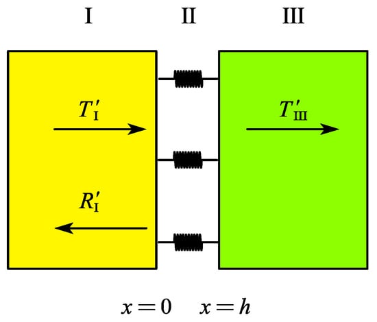
In the process of ultrasound propagation through multiple layers of media, reflections, and transmissions occur at acoustic boundaries due to the varying acoustic impedance of each layer. Thickness is one of the primary factors influencing the propagation of ultrasound. Different thicknesses of the medium result in varying reflection effects on ultrasound. Exploiting this phenomenon, the thickness of the oil film in bearings can be calculated through reflection coefficient analysis. Given the relatively thin nature of the oil film, the intermediate oil film layer is simplified as a lightweight spring [26], as illustrated in Figure 1. I and III are the media on both sides of the oil film, and II is the oil film layer. Yellow and green only represent the medium on both sides of the oil film and have no actual meaning. The material parameters are shown in Table 1.

According to the propagation characteristics of elastic waves in a medium, the displacement and stress of longitudinal waves are given by [27]:
The transmission of sound waves between different media requires continuity of displacement and stress at the interface between these media, considering and as the same boundary. It is understood that the continuous propagation of elastic waves necessitates equal displacement and stress on both sides of and . Neglecting the inertial factors of the oil film and assuming the amplitude of the incident sound wave is 1, the calculation formula for the acoustic reflection coefficient in the spring model is obtained [28].
This leads to the relationship between the reflection coefficient in the spring model and the oil film thickness [29].
3. Establishment of Finite Element Model
The properties of a solid are governed by the differential equations, which control phenomena such as the propagation of sound waves and deformation, along with other factors influencing substantial transformations. The equation is represented as follows:
In the bearing structure, a coupled interface exists between solid and liquid. It requires simultaneous consideration heat-transfer equation and the fluid heat-transfer equation to control the transfer of heat within the bearing. The heat-transfer equation in the solid is represented as follows:
The heat-transfer equation for the fluid is represented as follows in Equation (7), with its basic form being similar to the heat-transfer equation for solids.
By jointly controlling the aforementioned differential equations, the influence of changes in the oil film thickness of bearings on the ultrasound reflection coefficient under different temperature conditions is determined. This information establishes a formula for calculating the reflection coefficient under temperature compensation.
Ultrasound excitation signals typically use single-level or multi-level digital pulse signals. However, when propagating through multi-layered media, the output form of such pulse signals exhibits lower parameter accuracy. It contains numerous high-order harmonics, impacting the simulation accuracy of sound wave transmission and failing to meet simulation requirements. Therefore, a modulated sine function is chosen to exclude substantial interference from clutter in the detection signal, as shown in Equation (8).
Due to the significant computational time required for three-dimensional models in COMSOL, this model only considers the propagation of sound waves on a plane. A two-dimensional finite element model is established based on bearing data, and the material and boundary conditions of the finite element model are set as shown in Figure 2.
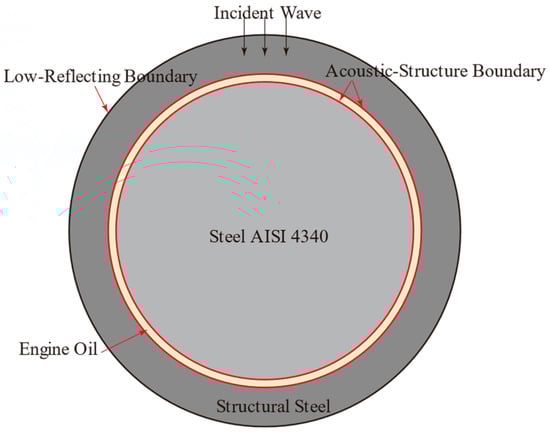
The model only analyzes the characteristics of the first echo; thus, it is necessary to eliminate the interference of multiple echoes on the measurement results. The Low-Reflecting Boundary (LRB) is commonly used to remove the interference of multiple reflected waves on the normal propagation of acoustic waves within the model. When the acoustic wave propagates to the boundary, the LRB ensures that the wave does not reflect in the time-domain or frequency-domain analysis. It acquires material data from the domain to create a perfect impedance match for pressure waves and shear waves.
When acoustic waves propagate in solids and fluids, their governing equations differ. When the acoustic wave propagates to the coupled boundary between solid and fluid, it is necessary to establish a coupling relationship to calculate the propagation of the acoustic wave at the coupled boundary. The Acoustic-Structure Boundary is used to couple pressure acoustic models with any structural component. This functionality couples with solid mechanics, elastic waves, shells, layered shells, membranes, and multibody dynamics interfaces. The coupling includes fluid loads on the structure and structural accelerations experienced by the fluid. For thin internal structures with fluid on both sides, such as shells or membranes, a slot is added in the pressure variable, and attention is paid to coupling the upper and lower sides.
Considering the need for efficient calculations while ensuring convergence during finite element computations, it is crucial to optimize computational efficiency. In finite element mesh generation, the mesh should be refined at the contact interfaces between different media based on the speed of sound in different media and the contact positions between media. Therefore, reasonable refinement of the mesh is required at various contact interface locations. When the mesh size is set between 1/6 and 1/5 of the wavelength, the relative error of the computed results is relatively small, proving that a mesh size between 1/6 and 1/5 of the wavelength is the optimal mesh density.
However, for the grids between the contact areas of different media layers, the mesh needs to be appropriately reduced, as reflections and transmissions of sound waves on the contact surface need to be calculated with high precision. The relative error approaches zero when the mesh size is less than 1/10 of the wavelength. Considering the computational time, a mesh size of 1/10 of the wavelength is chosen for these contact areas [22,30].
The model employs fully coupled transient methods, determining the wavelength of incident acoustic waves based on the mesh partition of the finite element model, ensuring convergence of the model within a certain range. By adjusting the boundary conditions of the model, convergence of the acoustic wave propagation at the boundary is ensured. Within the bearing model, there are multiple physics field couplings. The generalized α method within the implicit solver is employed for time stepping. The solver utilizes a free time step while determining the maximum step size to be . The backward Euler method is set with a safety factor of 20 for linear elements. Residuals of each physics field tend to stabilize during computation, and the convergence plot in COMSOL exhibits a smooth trend, indicating good convergence of the model and correct convergence condition settings.
4. Simulation Results Analysis
4.1. Analysis of Reflected Ultrasonic Signals at Different Temperatures
After performing Fourier transform on the reflected ultrasonic waves, the amplitude and phase of the reflected signal can be obtained. The reflection coefficient of the oil film is typically calculated using the reference signal and the reflected signal after Fourier transformation. Considering the temperature factor, the reflected ultrasonic wave at 20 °C is chosen as the reference signal, while the reflected ultrasonic waves under other temperature conditions are used as the reflected signals [31].
In ultrasonic measurement of bearing oil film thickness, there are three models involved: the spring model, the phase shift model, and the resonance model. Depending on the thickness of the oil film, the appropriate model is selected to calculate the oil film thickness. Since the effect of temperature on the signal characteristics corresponding to different oil film thicknesses is unknown, oil films with thicknesses of 20 μm and 100 μm are selected for analysis to assess the impact of temperature on the reflected acoustic wave signal. The 20 μm thick oil film exhibits characteristics of both the spring model and the phase shift model, while the 100 μm thick oil film presents characteristics of the resonance model. Therefore, the oil film with a thickness of 100 μm is chosen for the analysis and calculation of temperature interference.
Setting the oil film thickness to 20 μm, the model is configured with temperatures of 30 °C, 50 °C, 70 °C, 90 °C, and 110 °C in the solid and fluid heat transfer modules, and the computation of reflected ultrasonic waves is performed. The resulting time-domain signals are shown in Figure 3.
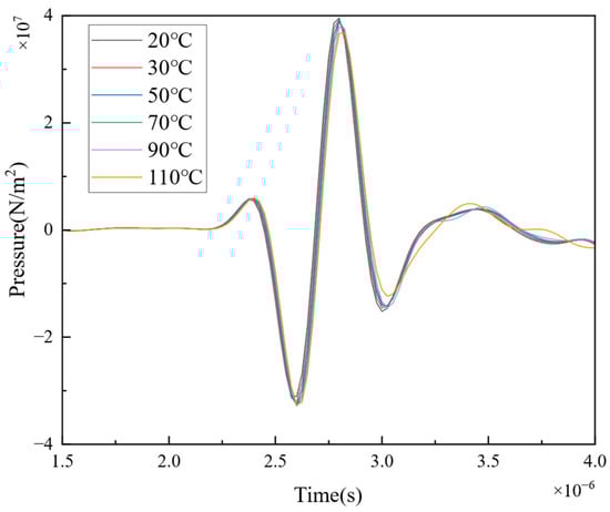
Figure 3.
The influence of temperature on acoustic signals under the condition of a 20 μm thick oil film.
According to Figure 3, it can be observed that the amplitude of the reflected ultrasonic wave remains relatively unchanged as the temperature increases. However, the phase gradually shifts to the right. Performing Fourier transform on the data yields the results shown in Figure 4a,b. The change in the amplitude of the reflected ultrasonic wave in the frequency domain follows a similar pattern to its time-domain counterpart, with minimal and localized variations that make it challenging to discern the impact of temperature on the amplitude. The phase of the reflected ultrasonic wave exhibits a regular variation in the frequency range, with the phase trend gradually shifting to the left as the temperature increases within the 6 MHz frequency range. The phase signal change is more pronounced than the amplitude signal.
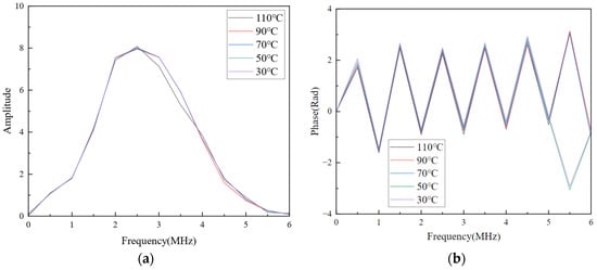
By substituting the signal information from Figure 4 into Equations (8) and (9), the amplitude and phase of the reflection coefficient in the frequency domain under the influence of temperature on the reflected ultrasonic wave for a 20 μm oil film thickness can be obtained, as shown in Figure 5. Figure 5a represents the amplitude of the reflection coefficient, where most of the reflection coefficients are entwined within the frequency range, making it challenging to analyze the impact of temperature on the reflected ultrasonic wave signal from the amplitude of the reflection coefficient. Figure 5b represents the phase of the reflection coefficient, and it can be observed that the phase of the reflection coefficient varies significantly under different temperature conditions. Moreover, the phases of the reflection coefficients are independent of each other, without entanglement or intertwining phenomena. The impact of temperature on the reflected ultrasonic wave can be more clearly reflected through the variation in the reflection coefficient phase.
Setting the oil film thickness in the finite element model to 100 μm, and keeping other conditions unchanged, the impact of temperature on the reflected ultrasonic wave is recalculated. The changes in the time-domain-reflected ultrasonic wave signals obtained from the finite element calculation are shown in Figure 6. Similar to the pattern observed with a 20 μm thick oil film, the amplitude of the reflected ultrasonic wave remains relatively unchanged when the temperature increases. However, the phase of the ultrasonic wave signal gradually shifts to the right as the temperature increases.
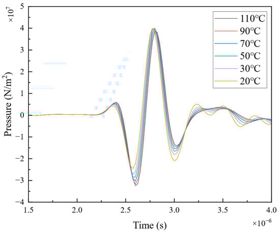
Figure 6.
The influence of temperature on acoustic signals under the condition of a 100 μm thick oil film.
After performing Fourier transform on the time-domain signals, frequency-domain signal images are obtained, as shown in Figure 7. Figure 7a represents the amplitude image of the reflected ultrasonic wave, while Figure 7b represents the phase image of the reflected ultrasonic wave.
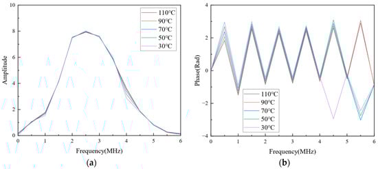
According to Figure 7, the variation in the amplitude of the reflected ultrasonic wave in the frequency domain follows a similar pattern to its time-domain counterpart. The amplitude changes are less pronounced, and the degree of amplitude variation is much smaller than that under the condition of a 20 μm oil film thickness. It is challenging to discern the impact of temperature on the reflected ultrasonic wave from the amplitude of the reflection coefficient. The phase of the reflected ultrasonic wave exhibits a regular variation in the frequency range, with the phase signal gradually shifting to the left as the temperature increases within the given range. The phase signal shows a regular and systematic change within the frequency range. Compared to the amplitude signal, the phase signal provides more compelling information, and its acquisition is relatively more straightforward, requiring less computational effort.
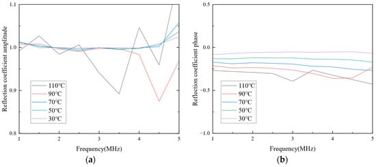
To demonstrate the influence of temperature on the phase of the ultrasonic wave, the reflection coefficient is used to characterize the relationship between the temperature and the reflected ultrasonic wave. Substituting the frequency-domain signals obtained after Fourier transform from Figure 7 into Equations (8) and (9), the amplitude and phase of the reflection coefficient in the frequency domain under the influence of temperature on the reflected ultrasonic wave for a 100 μm oil film thickness can be obtained, as shown in Figure 8.
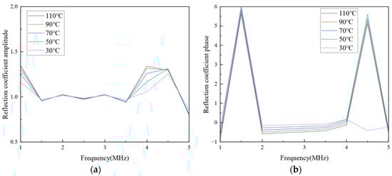
Figure 8a represents the amplitude of the reflection coefficient in the frequency domain. Compared to Figure 5a, the entanglement of this reflection coefficient amplitude is lighter. However, due to the small degree of variation in the amplitude of the reflection coefficient within the frequency range, it remains challenging to judge the impact of temperature on the reflected ultrasonic wave from the amplitude. Figure 8b represents the phase of the reflection coefficient in the frequency domain. There is a noticeable difference in the phase of the reflection coefficient under different temperature conditions. The phase of the reflection coefficient within this range can be used to establish the relationship between the reflected ultrasonic wave and temperature. In the 2–4 MHz range, the variation in the phase of the reflection coefficient is relatively regular. With the increase in temperature, the phase of the reflection coefficient gradually decreases, consistent with the trend of signal changes in the time domain. However, it provides a more straightforward way to obtain relationship information.
Through simulations under the coupling conditions of reflected ultrasonic waves and temperature fields with oil film thicknesses of 20 μm and 100 μm, it can be observed that the temperature variation has minimal impact on the amplitude of the reflected ultrasonic wave. However, it does specifically affect the phase of the reflected ultrasonic wave. With the increase in temperature, there is a trend of overall rightward shift in the reflected ultrasonic wave signal, indicating that temperature influences the phase relationship of the reflected ultrasonic wave. For the 20 μm oil film thickness condition, the spring model and phase shift model control the characteristics of the reflected ultrasonic wave. In contrast, for the 100 μm oil film thickness condition, the resonance model holds the characteristics of the reflected ultrasonic wave. The simulation results also indicate that the effect of temperature on the reflected ultrasonic wave is independent of the model containing the reflected ultrasonic wave. In other words, when analyzing the impact of temperature on the reflected ultrasonic wave, there is no need to consider the influence of oil film thickness on the reflected ultrasonic wave.
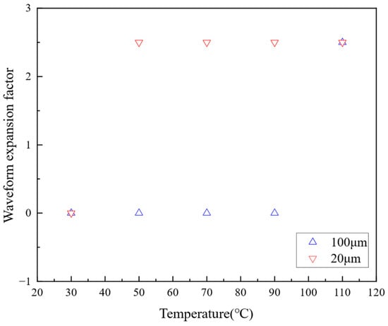
Because temperature affects the phase and amplitude of acoustic signals but does not impact the overall form of the signals, the degree of temperature influence on the signals can be analyzed through amplitude attenuation and waveform expansion factors. The amplitude attenuation factors and waveform expansion factors under the conditions of 20 μm and 100 μm oil film thickness are shown in Figure 9 and Figure 10, respectively.
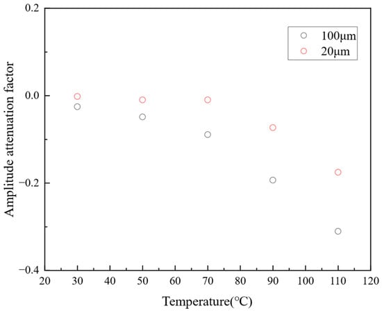
The amplitude attenuation factor is employed to analyze the trend of amplitude changes between signals, which are calculated by comparing the amplitude of the original signal with that of the transformed signal. Figure 9 shows that with the increase in temperature, the amplitude attenuation factor gradually decreases, indicating a reduction in amplitude compared to the original signal for the transformed signal.
The waveform expansion factor is utilized to analyze the trend of time difference changes between signals, calculated by determining the time difference between the peak values of the original signal and the transformed signal. Figure 10 shows that the waveform expansion factor for the 100 μm oil film thickness increases with rising temperature, reaching a plateau when the temperature exceeds 30 °C. The 20 μm oil film thickness waveform expansion factor shows no significant change below 90 °C due to the giant time step in the finite element calculation. Further refinement of the time step can yield more accurate waveform expansion factors. By analyzing the existing waveform expansion factors, it can be inferred that the peak values of the reflected acoustic signals gradually shift to the right as the temperature increases.
In the above analysis of the frequency and time domain characteristics of the signals, it has been demonstrated that temperature changes affect both the amplitude and phase of the reflected acoustic signals. The next step will involve compensating for these temperature-induced effects on the reflected acoustic signals to improve the accuracy of oil film thickness measurements.
4.2. Compensation of Reflected Acoustic Signals
The temperature variation has a significant impact on the acoustic properties of the medium. The density and speed of sound of the material jointly control acoustic properties. Compensating for the reflected acoustic signals involves adjusting the medium’s density and speed of sound. For lubricating oil compensation, Dowson and others proposed the following compensation formula.
Table 2 shows the variation function of the sound velocity and density of the medium at different temperatures. The variation in the density and sound velocity of the medium at different temperatures in COMSOL follows this functional trend. When calculating the thickness of the bearing oil film based on the acoustic reflection coefficient, it is necessary to consider the density and sound velocity of the medium. Usually, when calculating the thickness of the oil film, the influence of the bearing temperature on the reflection coefficient is not considered, and the actual density and sound velocity do not match the theoretical density and sound velocity. Correcting the medium density and sound velocity in COMSOL can compensate for the reflected acoustic signal. In practice, adjusting the incident acoustic signal can compensate for the reflected acoustic signal at different temperatures [23].
Table 2.
The density and speed of sound of the medium at different temperatures [23]. Reproduced with permission from Yaping Jia, Tonghai Wu, Pan Dou and Min Yu, Wear; published by Elsevier, 2024.
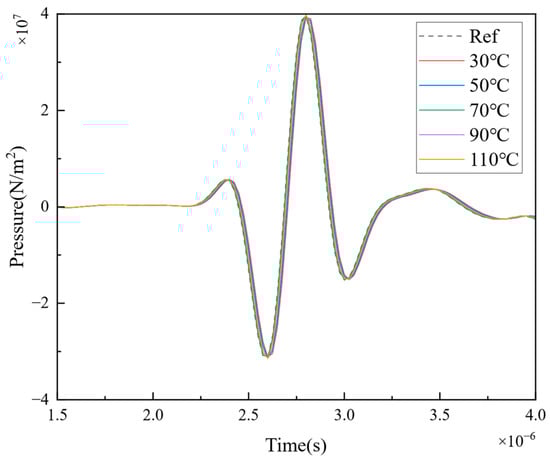
In COMSOL, the parameters of each material were adjusted according to the functions in Table 2, and finite element calculations were conducted again. The time-domain reflection acoustic signals are shown in Figure 11. In the figure, the reflected acoustic signals at various temperatures, after compensation, are nearly overlapping, demonstrating that compensating for the density and speed of sound is a practical approach to enhance measurement accuracy.
The Fourier-transformed signals after compensation are presented in Figure 12, illustrating their amplitude and phase spectra.
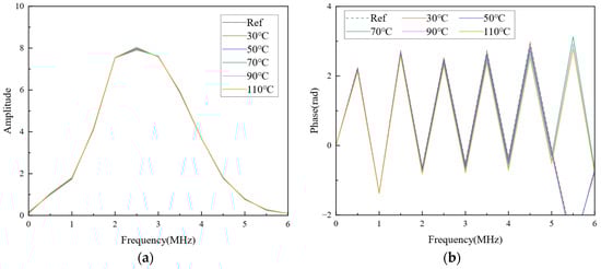
The calculated reflection coefficient amplitude and phase after compensation are shown in Figure 13. The amplitude curves of the reflection coefficient are closely aligned and indistinguishable between different temperatures. Compared to uncompensated signals, the compensated curves are numerically closer, making it nearly impossible to discern the impact of temperature on the reflection ultrasonic signals based on the reflection coefficient amplitude alone. In the compensated reflection coefficient phase, it is evident that the temperature-induced phase lag effect persists, but its magnitude is reduced. The compensated reflection coefficient phase is less than −0.25, half of the uncompensated reflection coefficient phase. This demonstrates the effectiveness of paying for density and speed of sound in the frequency domain. For practical oil film thickness measurements that do not require extremely high precision, temperature compensation for the medium’s density and speed of sound is sufficient to meet basic measurement requirements.
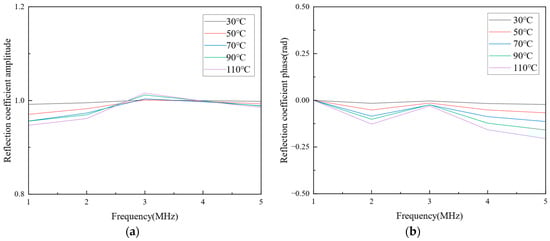
Figure 13.
The frequency domain reflection coefficient of the compensated signals: (a) amplitude, (b) phase.
In the time domain, the signals’ amplitude decay factor and waveform expansion factor are depicted in Figure 14. The maximum difference between amplitude decay factors is 0.0012, indicating that the amplitudes of the compensated signals between different temperatures remain almost unchanged. Due to the enormous time step, the waveform expansion factor of the compensated signals does not change, making it impossible to assess the correlation between waveform signals using the waveform expansion factor.
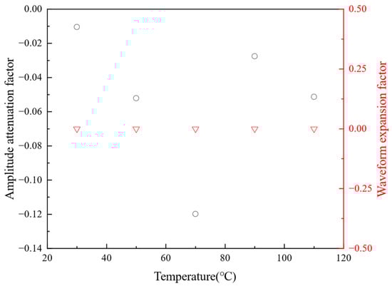
Figure 14.
The trends of amplitude decay factors and waveform expansion factors for the compensated signals.
The feasibility of improving the accuracy of oil film thickness measurement by compensating for density and speed of sound under temperature variations has been demonstrated through the characteristics of signals in both time and frequency domains. Depending on temperature changes, the relationship function between the density and speed of sound for solid media is represented by Equation (11).
The relationship function between density and speed of sound in liquid media is given by Equation (12).
Equations (11) and (12) represent functions describing the relationship between temperature and density, and temperature and speed of sound, respectively. The reflection coefficient is related to the medium’s density and speed of sound. A relationship function between the reflection coefficient and temperature is established, considering temperature as the independent variable. As the temperature changes, the medium’s density and speed of sound change synchronously in the equation to avoid computational errors arising from discrepancies between actual and theoretical densities and speeds of sound. The formula for calculating the compensated reflection coefficient is given by Equation (13).
In the time domain, compared to the reflected acoustic wave signal without temperature compensation, the compensated signal exhibits similar amplitudes, and the trend of phase shift is less noticeable. By calculating the amplitude attenuation factor and waveform expansion factor of different temperature waveforms, it is observed that the factors of the compensated signal tend to approach 0, indicating a convergence of different signals. In the frequency domain, judging the effect of temperature on the reflected acoustic wave based on the trend of amplitude change in the reflection coefficient is difficult. However, the phase of the reflection coefficient varies significantly with the temperature, with an upward shift in temperature causing a downward shift in the phase of the reflection coefficient. Through signal analysis in both the time and frequency domains, the effectiveness of temperature compensation for the reflected acoustic wave signal is demonstrated. This technique can be effectively applied to the measurement of bearing oil film thickness under various temperature conditions, thereby improving the accuracy of bearing oil film thickness measurement.
5. Compensation of Reflection Coefficients in Sliding Bearings under Multiple Temperature Conditions
During the sheet rolling process, variations in rolling force lead to different shear forces on the lubricating oil in the rolling mill bearings, resulting in varying temperatures of the bearing oil film. Under normal rolling loads, bearing temperatures typically range from 45 to 55 °C. If the bearing temperature exceeds this range, wear and scuffing may occur, and so temperatures must be maintained within the normal range to extend the working life of the bearings. A three-dimensional finite element model is established using COMSOL, incorporating modules such as Heat Transfer in Films Interface, Hydrodynamic Bearing Interface, Solid Mechanics Interface, Heat Transfer in Solids Interface, and coupling through the Multiphysics Branch with the inclusion of the Thermal Expansion module. This model simulates the bearings’ temperature and oil film thickness variations under different pressure conditions.
Different journal loads are set in the hydrodynamic bearing based on different rotational speed conditions to calculate the oil film thickness and temperature under various loads. The oil film thickness and temperature of the bearing under different loads are shown in Figure 15. It can be observed that there is a linear relationship between the bearing oil film thickness and the bearing load, with the oil film thickness decreasing as the load increases. The bearing oil film temperature shows a quadratic function relationship with the load, with the oil film temperature increasing as the load increases.
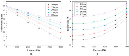
Figure 15.
Variations in oil film thickness and temperature under different rotational speeds: (a) pressure–film thickness, (b) pressure–temperature.
The fitting functions for pressure–temperature and pressure–film thickness are given by Equation (14). Based on these appropriate functions, temperatures and film thicknesses under different pressure conditions can be calculated, avoiding the inefficiency caused by multiple simulations. This demonstrates the functional relationship between pressure, temperature, and film thickness in actual bearings. When measuring bearings in a factory setting, this fitting function can be utilized to calculate and analyze oil film thickness under different conditions.
The coefficients in Equation (14) are listed in Table 3.
Considering the variations in density and sound speed induced by temperature, the reflection coefficients of the oil film under different pressure conditions are calculated based on the equation. Furthermore, the reflection coefficients after compensation for density and temperature are shown in Figure 16.
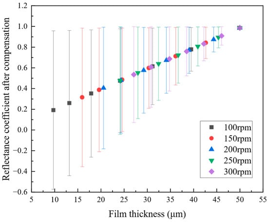
The error values between uncompensated reflection coefficients and compensated reflection coefficients are shown in Figure 17. The errors exhibit a linear trend between different oil film thicknesses, and the error gradually decreases with the increase in oil film thickness.
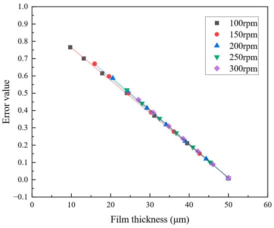
When the oil film thickness is less than 35 μm, there is a significant error between the reflection coefficients, making it impractical to calculate the oil film thickness changes using uncompensated reflection coefficients. However, when the oil film thickness exceeds 35 μm, the error between the reflection coefficients is relatively tiny. When measurement precision is not critical, uncompensated reflection coefficients can be used to calculate the oil film thickness. In cases of thin oil film, most of the acoustic waves transmit through the oil film without significant reflection at the interface with steel. Therefore, the reflection coefficient for a thin oil film is small. As the temperature increases, the density and speed of sound for the oil film and steel are significantly affected, resulting in increased reflection coefficients. This effect impacts the measurement of oil film thickness. Conversely, in the case of a thick oil film, most acoustic waves reflect at the oil film–steel interface, with only a tiny portion transmitting through. Consequently, the influence of temperature on the reflection coefficients is minimal in this scenario, resulting in a slight difference between the reflection coefficients under different temperatures. The fitted function for the reflection coefficient error in Figure 17 is given by Equation (15).
The coefficients of the fitted function are provided in Table 4.
The fitting function of the reflection coefficient error indicates that the temperature’s influence on the reflection coefficient exhibits an exponential change, i.e., the bearing pressure shows an exponential change in its effect on the reflection coefficient. Figure 18 shows the variation between bearing pressure and reflection coefficient error.
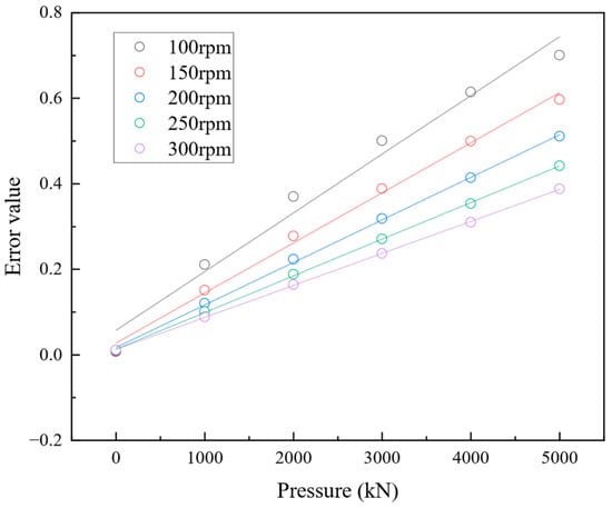
The relationship between bearing pressure and error values of the reflection coefficient is also an exponential function. Under the known conditions of bearing pressure, after measuring the reflection coefficient of the bearing oil film, the error in the reflection coefficient can be compensated using Equation (16), avoiding the calculation errors caused by unknown oil film thickness and distribution.
The coefficients of the fitting function are shown in Table 5.
According to Equation (16), the reflection coefficient error of the oil film thickness can be calculated under any bearing pressure conditions. When the bearing pressure exceeds a certain level, using this formula to calculate the reflection coefficient error becomes less significant.
The mathematical model’s goodness of fit is analyzed using the coefficient of determination , where a value approaching 1 indicates a good fit. However, is greatly influenced by the independent variables, and having a large number of independent variables may render ineffective. Therefore, the adjusted coefficient of determination, which considers the degrees of freedom, is used to characterize the fit of the mathematical model. The and adjusted of the aforementioned mathematical model are presented in Table 6. As the coefficients in Table 6 approach one, this indicates an excellent fit of the mathematical model, suggesting that it can be used to compensate for errors in the reflection coefficients under multiple temperature conditions, thereby achieving compensation in the bearing model measurement.
6. Conclusions
This paper introduces an error compensation method for measuring oil film thickness using ultrasonic waves at different temperatures. The process is applied to measure the oil film thickness of bearings at various temperatures. Conclusions are drawn through the analysis of finite element models under different temperature conditions, specifically focusing on the calculation results of the bearing oil film acoustic reflection coefficients.
- (1)
- Temperature is crucial to the measurement of the acoustic reflection coefficient in bearing oil film thickness. As the temperature increases, the phase of the reflected sound wave lags and the amplitude gradually decreases. This phenomenon is verified through analysis in the time and frequency domains. Therefore, when accurately measuring the thickness of bearing oil film, it is necessary to consider the impact of temperature on the density and sound speed of the medium and compensate for the reflection coefficient.
- (2)
- By adjusting the density and sound speed, the measurement model of the oil film reflection coefficient under multiple temperature conditions was compensated. The time-domain simulation results showed that in the compensated model, the reflected sound waves almost overlapped, with small changes in amplitude attenuation factors, but there was still a lag in phase. In the frequency domain, the reflected sound wave amplitudes under different temperatures were similar and remained stable. This presented a challenge for solving the phase lag problem.
- (3)
- Based on signal compensation under multiple temperature conditions, a model of liquid dynamic pressure bearing was established, and the changes in the oil film of the bearing under different load conditions were analyzed. As the load increases, the temperature of the oil film increases and the thickness of the oil film decreases. The simulation results show that there is an error between the thickness of the oil film and the reflection coefficient. By establishing an error model, the calculation problem of reflection coefficient error is solved, which lays a foundation for analyzing the influence of temperature on reflection coefficient error.
Based on the findings from the research above, a method for detecting the thickness of hydrodynamic-bearing oil films under multiple temperature conditions has been established. This method addresses the errors introduced by temperature variations in oil film thickness measurements, ensuring the feasibility of measuring hydrodynamic bearing oil film thickness under different temperature conditions. It improves the accuracy of oil film thickness detection that may be affected by temperature issues, providing theoretical support for industrial applications.
Author Contributions
Conceptualization, F.S. and B.S.; methodology, B.S.; software, Y.B.; validation, B.S., S.W. and Y.H.; formal analysis, W.L.; investigation, N.K.; resources, Y.B.; data curation, F.M.; writing—original draft preparation, F.S. and B.S.; writing—review and editing, Y.H. and Z.L.; visualization, W.L.; supervision, S.W.; project administration, F.S.; funding acquisition, S.W., N.K. and Y.B. All authors have read and agreed to the published version of the manuscript.
Funding
This research was funded by the Science and Technology Planning Project of Inner Mongolia Autonomous Region, grant number 2022YFSH0126 and by the Fundamental Research Funds for Inner Mongolia University of Science & Technology, grant number 2023QNJS072, and by the Natural Science Foundation of Inner Mongolia Autonomous Region, grant number 2023ZD12, and by theBasic scientific research business expenses project of universities directly under the Inner Mongolia Autonomous Region, grant number 2024YXXS058.
Data Availability Statement
Please contact the corresponding author for data.
Acknowledgments
We would like to thank the Science and Technology Planning Project of Inner Mongolia and the Fundamental Research Funds for Inner Mongolia University of Science & Technology for sponsoring this research. We also appreciate the support of the School of Mechanical Engineering at Inner Mongolia University of Science & Technology for this study. Additionally, we thank the editors and reviewers for their assistance with this paper. In this paper, a large language model was used to optimize the grammatical content of the article.
Conflicts of Interest
Author Fengchun Miao was employed by the company Inner Mongolia North Heavy Industry Group Co., Ltd. The remaining authors declare that the research was conducted in the absence of any commercial or financial relationships that could be construed as a potential conflict of interest.
Nomenclature
| Symbol | Unit | |
| m | Displacement of elastic waves. | |
| Hz | Angular frequency of incident sound wave. | |
| - | Amplitudes of the incident waves. | |
| - | Amplitudes of the reflected waves. | |
| m/s | Speed of sound. | |
| kg/(m2·s) | Acoustic impedance. . | |
| - | Acoustic reflection coefficient. | |
| kg/m3 | Density. | |
| N/m | . | |
| Pa | Stress tensor. | |
| m/s | Velocity field defined at the velocity grid nodes. | |
| J/kg·°C | Solid heat capacity under constant pressure. | |
| N | Load vector. | |
| W | Heat source. | |
| W/(m·K) | Reliable thermal conductivity. | |
| W | Pressure work. | |
| W | Thermoelastic damping. | |
| m/s | Specified velocity on the boundary. | |
| W | Viscous dissipation. | |
| - | Amplitude of the reflection coefficient. | |
| s | Signal period. | |
| - | Amplitude of the reference signal in the frequency domain. | |
| - | Amplitude of the reflected ultrasonic wave in the frequency domain. | |
| rad | Phase of the reflection coefficient. | |
| - | Reflection coefficient of the reference signal in the frequency domain, typically taken as one. | |
| rad | Phase of the reference signal in the frequency domain. | |
| rad | Phase of the reflected ultrasonic wave in the frequency domain. | |
| kg/m3 | Density at temperature . | |
| rad | Phase of the reflection coefficient of the reference signal in the frequency domain, typically taken as 0. | |
| Pa−1 | Density–pressure coefficient. | |
| kg/m3 | Density at temperature . | |
| K−1 | Density–temperature coefficient. | |
| Pa−1 | Density–pressure coefficient. | |
| m/m/K | Thermal expansion coefficient. | |
| kg/m3 | Density varying with temperature. | |
| m/s | Speed of sound running with temperature. | |
| K | Temperature. | |
| kg/(m2·s) | Temperature-compensated acoustic impedance. | |
| - | Temperature-compensated reflection coefficient. | |
| N | Pressure applied to the bearing. | |
| m | Bearing oil film thickness. | |
| - | Reflection coefficient error. | |
| m | Temperature of the bearing oil film. |
References
- Peng, H.; Zhang, H.; Shangguan, L.; Fan, Y. Review of Tribological Failure Analysis and Lubrication Technology Research of Wind Power Bearings. Polymers 2022, 14, 3041. [Google Scholar] [CrossRef]
- Marko, M.D. The Impact of Lubricant Film Thickness and Ball Bearings Failures. Lubricants 2019, 7, 48. [Google Scholar] [CrossRef]
- Xu, F.; Ding, N.; Li, N.; Liu, L.; Hou, N.; Xu, N.; Guo, W.; Tian, L.; Xu, H.; Lawrence Wu, C.; et al. A review of bearing failure Modes, mechanisms and causes. Eng. Fail. Anal. 2023, 152, 107518. [Google Scholar] [CrossRef]
- Zhu, S.; Yuan, W.; Cong, J.; Guo, Q.; Chi, B.; Yu, J. Analysis of regional wear failure of crankshaft pair of heavy duty engine. Eng. Fail. Anal. 2023, 154, 107635. [Google Scholar] [CrossRef]
- Zhang, Y.; Wang, W.; Zhang, S.; Zhao, Z. Optical analysis of ball-on-ring mode test rig for oil film thickness measurement. Friction 2016, 4, 324–334. [Google Scholar] [CrossRef]
- Mu, B.; Qu, R.; Tan, T.; Tian, Y.; Chai, Q.; Zhao, X.; Wang, S.; Liu, Y.; Zhang, J. Fiber Bragg Grating-Based Oil-Film Pressure Measurement in Journal Bearings. IEEE Trans. Instrum. Meas. 2019, 68, 1575–1581. [Google Scholar] [CrossRef]
- Deng, Y.; Zhong, S.; Lin, J.; Zhang, Q.; Nsengiyumva, W.; Cheng, S.; Huang, Y.; Chen, Z. Thickness Measurement of Self-Lubricating Fabric Liner of Inner Ring of Sliding Bearings Using Spectral-Domain Optical Coherence Tomography. Coatings 2023, 13, 708. [Google Scholar] [CrossRef]
- Xie, K.; Liu, L.; Li, X.; Zhang, H. Non-contact resistance and capacitance on-line measurement of lubrication oil film in rolling element bearing employing an electric field coupling method. Measurement 2016, 91, 606–612. [Google Scholar] [CrossRef]
- Cheng, M.H.; Chiu, G.T.C.; Franchek, M.A. Real-Time Measurement of Eccentric Motion with Low-Cost Capacitive Sensor. IEEE/ASME Trans. Mechatron. 2013, 18, 990–997. [Google Scholar] [CrossRef]
- He, Y.; Wang, J.; Gu, L.; Zhang, C.; Yu, H.; Wang, L.; Li, Z.; Mao, Y. Ultrasonic measurement for lubricant film thickness with consideration to the effect of the solid materials. Appl. Acoust. 2023, 211, 109563. [Google Scholar] [CrossRef]
- Wang, J.; He, Y.; Shu, K.; Zhang, C.; Yu, H.; Gu, L.; Wang, T.; Li, Z.; Wang, L. A sensitivity-improved amplitude method for determining film thickness based on the partial reflection waves. Tribol. Int. 2023, 189, 109010. [Google Scholar] [CrossRef]
- Zhang, K.; Wu, T.; Meng, Q.; Meng, Q. Ultrasonic measurement of oil film thickness using piezoelectric element. Int. J. Adv. Manuf. Technol. 2018, 94, 3209–3215. [Google Scholar] [CrossRef]
- Dou, P.; Wu, T.; Luo, Z. Wide Range Measurement of Lubricant Film Thickness Based on Ultrasonic Reflection Coefficient Phase Spectrum. J. Tribol. 2019, 141, 031702. [Google Scholar] [CrossRef]
- Beamish, S.; Li, X.; Brunskill, H.; Hunter, A.; Dwyer-Joyce, R. Circumferential film thickness measurement in journal bearings via the ultrasonic technique. Tribol. Int. 2020, 148, 106295. [Google Scholar] [CrossRef]
- Beamish, S.; Dwyer-Joyce, R.S. Experimental Measurements of Oil Films in a Dynamically Loaded Journal Bearing. Tribol. Trans. 2022, 65, 1022–1040. [Google Scholar] [CrossRef]
- Dou, P.; Wu, T.; Luo, Z.; Yang, P.; Peng, Z.; Yu, M.; Reddyhoff, T. A finite-element-aided ultrasonic method for measuring central oil-film thickness in a roller-raceway tribo-pair. Friction 2022, 10, 944–962. [Google Scholar] [CrossRef]
- Jia, Y.; Dou, P.; Zheng, P.; Wu, T.; Yang, P.; Yu, M.; Reddyhoff, T. High-accuracy ultrasonic method for in-situ monitoring of oil film thickness in a thrust bearing. Mech. Syst. Signal Process. 2022, 180, 109453. [Google Scholar] [CrossRef]
- Wei, S.; Wang, J.; Cui, J.; Song, S.; Li, H.; Fu, J. Online monitoring of oil film thickness of journal bearing in aviation fuel gear pump. Measurement 2022, 204, 112050. [Google Scholar] [CrossRef]
- Gray, W.A.; Dwyer-Joyce, R.S. In-situ measurement of the meniscus at the entry and exit of grease and oil lubricated rolling bearing contacts. Front. Mech. Eng. 2022, 8, 1056950. [Google Scholar] [CrossRef]
- Dou, P.; Zou, L.; Wu, T.; Yu, M.; Reddyhoff, T.; Peng, Z. Simultaneous measurement of thickness and sound velocity of porous coatings based on the ultrasonic complex reflection coefficient. NDT E Int. 2022, 131, 102683. [Google Scholar] [CrossRef]
- Dou, P.; Zheng, P.; Jia, Y.; Wu, T.; Yu, M.; Reddyhoff, T.; Liao, W.; Peng, Z. Ultrasonic measurement of oil film thickness in a four-layer structure for applications including sliding bearings with a thin coating. NDT E Int. 2022, 131, 102684. [Google Scholar] [CrossRef]
- Shang, F.; Sun, B.; Zhang, H. Measurement of Air Layer Thickness under Multi-Angle Incidence Conditions Based on Ultrasonic Resonance Reflection Theory for Flange Fasteners. Appl. Sci. 2023, 13, 6057. [Google Scholar] [CrossRef]
- Jia, Y.; Wu, T.; Dou, P.; Yu, M. Temperature compensation strategy for ultrasonic-based measurement of oil film thickness. Wear 2021, 476, 203640. [Google Scholar] [CrossRef]
- Zhang, M.; Ma, X.; Guo, N.; Xue, Y.; Li, J. Calculation and Lubrication Characteristics of Cylindrical Roller Bearing Oil Film with Consideration of Thermal Effects. Coatings 2023, 13, 56. [Google Scholar] [CrossRef]
- Mo, H.; Hu, Y.; Quan, S. Thermo-Hydrodynamic Lubrication Analysis of Slipper Pair Considering Wear Profile. Lubricants 2023, 11, 190. [Google Scholar] [CrossRef]
- Tattersall, H.G. The ultrasonic pulse-echo technique as applied to adhesion testing. J. Phys. D Appl. Phys. 1973, 6, 819–832. [Google Scholar] [CrossRef]
- Achenbach, J.D. Wave Propagation in Elastic Solids; North-Holland Pub. Co.: Amsterdam, The Netherlands, 1973; p. 425. [Google Scholar]
- Reddyhoff, T.; Dwyer-Joyce, R.; Harper, P. Ultrasonic measurement of film thickness in mechanical seals. Seal. Technol. 2006, 2006, 7–11. [Google Scholar] [CrossRef]
- Zhu, J.; Li, X.; Beamish, S.; Dwyer-Joyce, R.S. An ultrasonic method for measurement of oil films in reciprocating rubber O-ring seals. Tribol. Int. 2022, 167, 107407. [Google Scholar] [CrossRef]
- Shang, F.; Sun, B.; Li, H.; Zhang, H.; Liu, Z.; Meng, X.; Jiang, L.; Xv, G. Detection Method for Bolt Loosening and Washer Damage in Flange Assembly Structures Based on Phased Array Ultrasonics. Res. Nondestruct. Eval. 2024, 1–27. [Google Scholar] [CrossRef]
- He, Y.; Gao, T.; Guo, A.; Qiao, T.; He, C.; Wang, G.; Liu, X.; Yang, X. Lubricant Film Thickness Measurement Based on Ultrasonic Reflection Coefficient Phase Shift. Tribology 2021, 41, 1–8. [Google Scholar]
Disclaimer/Publisher’s Note: The statements, opinions and data contained in all publications are solely those of the individual author(s) and contributor(s) and not of MDPI and/or the editor(s). MDPI and/or the editor(s) disclaim responsibility for any injury to people or property resulting from any ideas, methods, instructions or products referred to in the content. |
© 2024 by the authors. Licensee MDPI, Basel, Switzerland. This article is an open access article distributed under the terms and conditions of the Creative Commons Attribution (CC BY) license (https://creativecommons.org/licenses/by/4.0/).