Machine Learning-Based Prediction of Elastic Properties Using Reduced Datasets of Accurate Calculations Results

Abstract

In this paper, the applicability of machine learning for predicting the elastic properties of binary and ternary bcc Ti and Zr disordered alloys with 34 different doping elements is explored. The original dataset contained 3 independent elastic constants, bulk moduli, shear moduli, and Young’s moduli of 1642 compositions calculated using the EMTO-CPA method and PAW-SQS calculation results for 62 compositions. The architecture of the system is made as a pipeline of a pair of predicting blocks. The first one took as the input a set of descriptors of the qualitative and quantitative compositions of alloys and approximated the EMTO-CPA data, and the second one took predictions of the first model and trained on the results of the PAW-SQS calculations. The main idea of such architecture is to achieve prediction accuracy at the PAW-SQS level, while reducing the resource intensity for obtaining the training set by a multiple of the ratio of the training subsets sizes corresponding to the two used calculation methods (EMTO-CPA/PAW-SQS). As a result, model building and testing methods accounting for the lack of accurate training data on the mechanical properties of alloys (PAW-SQS), balanced out by using predictions of inaccurate resource-effective first-principle calculations (EMTO-CPA), are demonstrated.

1. Introduction

Disordered titanium and zirconium body-centered cubic (bcc) alloys are highly demanded materials for different applications. For example, they are used in biomedical devices such as bone implants for every part of the body due to their high biocompatibility and corrosion resistance [1,2]. Although titanium-based alloys usually surpass zirconium-based ones in mechanical properties, the latter can be used, for example, for implants that provide less noise in magnetic resonance imaging procedures due to much lower magnetic susceptibility [3]. Some Ti and Zr alloys, including a Ti-Zr solid solution, demonstrate shape-memory behavior, and can be used for designing medical tools and other devices, similarly to nitinol [4]. Examples of multicomponent bcc alloys for medical applications are Ti-13Nb-13Zr, Ti-35Nb-5Ta-7Zr, Ti-29Nb-13Ta, and Ti-24Nb-4Zr-8Sn. Some titanium alloys, such as Ti-13V-11Cr-3Al, are used in the aerospace industry due to their softness in the bcc phase and the ability to subsequently strengthen during aging. β-alloys such as Ti-15V-3Sn-3Cr-3Al, Ti-10V-2Fe-3Al, and Ti-5Al-5V-5Mo-1Cr-1Fe have low flow stresses, which facilitates metal processing, while Ti-15Mo-2.7Nb-3Al-0.2Si and Ti-35V-15Cr exhibit superplastic behavior at stress rates below 10-5 s-1. Ti-5Al-5V-5Mo-3Cr-0.5Fe demonstrates high oxidation resistance and burn resistance. Ti-Mo and Ti-Nb alloys (for example, Ti with 40.5 at. % Nb) can also exhibit superelasticity. There is also a type of β-titanium alloy called gum metals, such as Ti-23Nb-0.7Ta-2Zr-1O (which may also include V and Hf), which has unique properties such as a low Young’s modulus of about 40 GPa with high tensile strength up to 2 GPa and exhibits superelasticity, or even superplasticity [5]. Available data on titanium and zirconium β-alloys show that materials based on them can have prominent properties. Considering the variety of possible alloying elements, it can be concluded that this class of materials represents a vast field of research and the search for new materials.

The elaboration of quantum-mechanical methods of computational materials science has led to the development of many implementations, including high-performance computing packages. Most calculations of the properties of disordered crystalline solids are resource-intensive tasks for computer clusters, which makes it difficult to search for new materials. Among the calculation methods within the framework of the electron density functional theory (DFT), the least resource-intensive ones can be distinguished, for example, the exact muffin-tin orbitals (EMTO) method with coherent potential approximation (CPA) [6], which is effective in modeling solid solutions. However, the electronic structure problem within this method is solved using the spherical approximation for the one-electron potential. Moreover, the EMTO-CPA is a single-site mean-field approximation. These approximations can lead to some inaccuracy. Indeed, it is well known that the bcc structure of pure titanium and zirconium is mechanically unstable at low temperatures. From the point of view of elastic properties, this should lead to strongly negative values of the elastic constant C’. However, in the EMTO-CPA method, this constant turns out to be close to zero for Ti and has a positive value for Zr. The more accurate but resource-intensive projector augmented wave method (PAW) [7] does not have such disadvantages [8,9]. However, in the case of solid solutions, it requires the use of the special quasi-random structures (SQS) method [10], which further increases the computational complexity as it involves supercells. Therefore, the reliability of the EMTO-CPA calculations must be verified in comparison with more accurate calculations. Such a comparison is demonstrated in work [11] for a set of titanium-based bcc binary alloys. Taking into account the difference in the performance and accuracy of the methods, the idea of applying supervised machine learning, which could compensate for the lack of calculated data of a more accurate method, logically arises.

Machine learning (ML) is vastly applied in the field of material science for different tasks, such as the prediction of mechanical, thermal, electrical, and other material properties including various effects and phase transitions. For these purposes, a training dataset for ML models can include crystal structure information, already-known experimental data, and data obtained via ab initio calculations and their combinations [12]. The application of machine learning in the context of first principles calculations has a distinct advantage over other applications of ML in materials science. Both theoretical calculations and machine learning are limited only by computing resources and are not limited by such factors as the availability of materials and the variety of experimental and analytical equipment. The reasonable application of machine learning to predict some properties can exponentially reduce the computational cost compared to ab initio calculations [13]. Typical features used for ML models for material science include representation of the chemical formula using a vector of elements presented in material, properties of materials such as elastic moduli, thermal expansion coefficient, electronegativity, or more complex parameters, such as Seeback or Peltier coefficients. Some features can be obtained through the statistics of the specified properties of the constituent elements, including averages, medians, maximal or minimal values, etc. [13,14], with respect to considered compositions. A set of features can be derived from the crystal structure, for example, the lattice parameter, space group, and the number of nearest neighbors.

The most accessible machine learning methods are often based on the use of training sets, which leads to an obvious data availability problem. Given this, machine learning on the results of theoretical calculations provides a significant advantage, since currently a significant amount of standardized data describing the results of ab initio calculations is available in the public domain [15,16,17,18,19]. There are many examples in the literature of using such databases for predicting properties and developing new materials. Thus, Tawfik et al. [20] used a dataset of 3112 compositions from the materials project database to predict the materials’ vibrational stability. The features used consisted of one-hot encoded symmetry groups, robust one-shot ab initio descriptors (ROSA), which describe elemental properties, and include different energy components (occupied and unoccupied energy levels, total kinetic, Fermi, exchange-correlation energies, etc.), bulk modulus, molar volume, and symmetry functions of atomic positions extracted from the results of calculations in the framework of density functional theory [21]. Paz Soldan Palma et al. [22] used calculated formation enthalpies from the materials project to determine materials stability in terms of convex hulls. Kruthika and Ravindran [23] extracted the data for 90 perovskites from materials project and ICSD databases to predict optoelectronic properties. Roy et al. [24] used data from the materials project for comparison with their results, obtained through classical molecular dynamics.

A number of examples of using machine learning to predict the elastic properties of disordered alloys are described in the literature. For example, in the work [25], artificial neural networks and support vector machine models were successfully used to predict the mixing enthalpy, Young’s modulus, and the ratio between the shear modulus and bulk modulus of Fe-Cr alloys. To describe the compositions of the training set in the feature space, the characteristics of the elements in their ground state were used, among which the atomic radii mismatch, average atomic volume, averaged valence electron concentration, total electronegativity, and ideal mixing entropy are mentioned. In the work [26], authors used the full potential Korringa–Kohn–Rostoker (FPKKR) method within the coherent potential approximation to construct a training set of 2555 high-entropy alloys for an elastic property prediction using linear regression and neural network models based on 316 descriptors. The paper by Kim et al. [27], incorporating EMTO-CPA and PAW-SQS calculations, describes the use of two separate gradient boosting models to predict the bulk and shear moduli of high-entropy alloys based on materials project data. For feature selection, the authors used the multi-objective optimized genetic algorithm proposed in [28,29]. The most important features found were descriptors based on the properties of the elements included in the resulting compositions, such as group number, cohesive energy, density, electronegativity, and atomic radius.

Notably, widely used structural descriptors [21] lose their importance to some extent when it comes to using machine learning for a set of materials limited to disordered alloys of a single type of symmetry. To predict the properties of such materials, a set of cost-efficient and universal features can be distinguished among the various methods of feature engineering, which are intended to be used in material property prediction based on the results of theoretical calculations. This group of features describes the properties related to the chemical composition of the investigated materials and includes the statistics of the properties of the elements that are part of the considered compositions, statistics of oxidation states, and many others [30].

Even with the mentioned calculated data availability, most material data used for machine learning fall under the category of small data. The PAW-SQS calculations for disordered structures are complex and time-consuming to create large databases. Thus, one of the significant problems in creating machine learning models for accurately predicting the properties of materials with a disordered structure is the lack of extensive training sets [31].

For the case of small data, there are several effective approaches mentioned in the literature. Transfer learning involves the transfer of knowledge gained from one task to improve learning on a different but related task. This strategy is particularly useful for small datasets as it allows models to benefit from pre-trained knowledge and patterns from larger datasets [32,33,34]. Another effective concept is ensemble learning, which combines multiple models to make predictions, often resulting in better performance than individual models. By aggregating predictions from diverse models, ensemble methods can mitigate the limitations of small datasets [35,36]. The active learning strategy involves iteratively selecting the most informative data points and incorporating them into the training set [37,38].

The combination of transfer and ensemble learning offers a powerful strategy to reduce the amount of resource-intensive calculations, and improve model robustness and predictive accuracy in machine learning applications for materials science. In the paper [39], the concept of transfer learning was implemented by leveraging data from the CALPHAD (calculation of phase diagrams) database to enhance the machine learning model for predicting the synthesizability of high-entropy ceramics. By combining general features with thermodynamic data from a less accurate calculation method (CALPHAD), the predictive ability of the ensemble random-forest regression model was improved, and demonstrated robustness in extrapolating outside the starting chemical space.

As noted above, ensemble methods are effective when handling tasks involving small data. Several tools can be highlighted among the available implementations: “CatBoost” [40], “XGBoost” [41], “LightGBM” [42], and “Gradient Boosting Machine” (GBM) [43], which are effective for small datasets as they can handle complex relationships in the data and prevent overfitting [31,36]. Thus, in the work [44] the described problem is solved for the case of predicting the basic d-spacing in materials for supercapacitors. By comparing XGBoost, support vector machine, and artificial neural network models, the authors demonstrated that the most effective model is gradient boosting.

Overall, the literature provides examples of solving problems of predicting the results of theoretical calculations based on reduced datasets. However, it can be noted that there is a lack of research relevant to the objectives of this work. In this work, to achieve high predictive ability at the PAW level, but at the same time using a relatively small number of results obtained by resource-intensive calculations, the basic idea of the gradient boosting algorithms, which consist of an improvement of predictions using an ensemble of weak predictors, was used. The models of this ensemble can be stage-wise arranged, where the prediction errors of one model are taken into account by the other one, allowing it to obtain more accurate predictions by learning from collective mistakes made by stacked models [45,46].

Considering the differences in the performance of the DFT calculation methods, the main task of this work was to develop a method for predicting the elastic properties of bcc alloys within both interpolation and extrapolation, i.e., when several concentration points are known, but more accurate knowledge of the values between them is required, and when completely new systems are predicted. In the case of extrapolation for these new systems, there were no fitting data used for model training.

In this work, a novel approach of augmenting the PAW-SQS reduced training data with EMTO-CPA calculations used for the stage-wise prediction is proposed. This approach aimed to enhance predictive ability in the task of predicting elastic properties, both supplementing the already-known concentration dependencies with new compositions, and predicting the properties of new bcc-alloys.

2. Materials and Methods

The selected properties of disordered alloys to predict include: three independent components of elastic tensor for the cubic crystal structure (C₁₁, C₁₂, C₄₄, C’ = (C₁₁ − C₁₂)/2), bulk modulus (B), Young’s modulus (E), and shear modulus (G). A detailed description of the methodology and results is available in the work [9,11]. All data used for the training sets were obtained as a result of ab initio calculations using two methods: EMTO-CPA [6,47] and PAW-SQS [7,10,48]. The effects of the dissolution of 3d, 4d, and 5d metals and Al, Ga, In, and Sn in the bcc Ti lattice (β-phase) were modeled within the framework of EMTO-CPA calculations. The PAW-SQS method was used to calculate the above set of properties for only a part of the bcc Ti-X alloys. For this dataset, the list of alloying elements X included 4d elements Nb, Mo, Tc, Ru, and Rh and 5d elements Ta, W, Re, Os, and Ir. The properties of binary zirconium-disordered alloys were calculated similarly in both methods. To further increase the training set, the indicated properties of Ti-X-Y ternary alloys, where X, Y = Ag, Al, Au, Co, Cr, Cu, Fe, Ga, Ge, Hf, In, Ir, Mn, Mo, Nb, Pd, Pt, Re, Rh, Ru, Sn, Ta, Tc, V, W, Zn, and Zr, were also calculated in the same manner as for binaries within the EMTO-CPA method.

In the EMTO-CPA method, the total charge density is obtained by an exact self-consistent solution of the one-electron Kohn–Sham equations for overlapping spherical muffin-tin (MT) potentials. The effective medium is constructed in such a way that the electron scattering off the effective atoms is averaged, as in the simulated disordered alloy. The self-consistent solution of a system of CPA equations was formulated in terms of the Green’s function. The disadvantages of this method are the absence of local relaxations and the use of the spherical MT potential. In the EMTO, s-, p-, d-, and f-orbitals were accounted for. The full charge density (FCD) was represented by a single-center expansion of the electron wave functions in terms of spherical harmonics with orbital angular moments l_FCD^max = 8. The integration in the irreducible part of the Brillouin zone was performed over a 29 × 29 × 29 grid of k points. The energy integration was carried out in the complex plane using a semi elliptic contour comprising 24 energy points. In order to determine the elastic constants C’ and C₄₄ within EMTO-CPA, orthorhombic (1) and monoclinic (2) volume-conserving distortions were applied, and the internal energy response to the six distortions sets (η = 0.00–0.05) [9] was calculated:

$$1+{\epsilon }_1=\left(\begin{array}{ccc}1+\eta & 0& 0\\ 0& 1-\eta & 0\\ 0& 0& \frac{1}{1-{\eta }^2}\end{array}\right)$$

(1)

$$1+{\epsilon }_2=\left(\begin{array}{ccc}1& \eta & 0\\ \eta & 1& 0\\ 0& 0& \frac{1}{1-{\eta }^2}\end{array}\right)$$

(2)

In the PAW method, exchange-correlation effects in an electron gas were taken into account within the density functional theory in the framework of the generalized gradient approximation (GGA) [49]. Short-range order parameters for the several neighboring coordination spheres of generated SQS supercells were optimized to be close to zero [10]. For bcc alloys, 4 × 4 × 4 128-atom SQS supercells were constructed. The integration of the Brillouin zone was performed over the grid of 4 × 4 × 4 k points. The number of plain waves considered was determined by cutoff energy of 450 eV. To obtain elastic constants within the PAW-SQS calculations, the following deformation matrix was used [50]:

$$1+\epsilon =\left(\begin{array}{ccc}1+\eta & \frac{\eta }{2}& 0\\ \frac{\eta }{2}& 1& 0\\ 0& 0& 1\end{array}\right)$$

(3)

The magnitude of the deformation (η) varied from −0.02 to +0.02 with a step of 0.01. Accordingly, elastic constants are determined from the following stress–strain relationships [50]:

$$C_{11}=\frac{\partial {\sigma }_{xx}}{\partial \eta }, C_{12}=\frac{\partial {\sigma }_{yy}}{\partial \eta }{, C}_{44}=\frac{\partial {\sigma }_{xy}}{\partial \eta }$$

(4)

To estimate the B and G, the Voigt–Reuss–Hill procedure was used [51]. The Young’s modulus E was derived according to the following relations [52]:

$$B=\frac{C_{11}+2C_{12}}{3}, G=\frac{1}{2}\left(\frac{5C_{44}\left(C_{11}-C_{12}\right)}{4C_{44}+3\left(C_{11}-C_{12}\right)}+\frac{C_{11}-C_{12}+3C_{44}}{5}\right)$$

(5)

$$E=\frac{9BG}{3B+G}$$

(6)

It is important to note that the calculations within the framework of the EMTO-CPA method are low-cost, while PAW-SQS requires much more computational resources. For example, calculating the elastic constant C₁₁ of one composition within the EMTO-CPA framework requires about 50 core hours, and about 1400 core hours within the PAW-SQS.

The input data for both models were represented by a set of predicted data and a composition expressed in contained elements and their atomic concentrations.

In detail, the EMTO-CPA dataset consists of information describing calculated properties for 2 pure elemental samples (Ti, Zr), 615 binaries, and 1025 ternary compositions. Base element concentrations for binaries are presented in the range from 50 to 95 with the step of 5 at. %. Dopants of binaries presented by 34 elements: 33 for Ti-based alloys and 29 for Zr-based alloys. Ternary compositions are presented by 41 Ti-based systems. Base element concentrations for ternaries are presented in the range from 50 to 90 with the step of 10 at. %, and the second and third element concentrations for ternaries are presented by the ranges from 5 to 45 with the step of 5 at. %.

The PAW-SQS dataset describes the calculated properties for pure elements (Ti, Zr) and 60 binary compositions of 10 dopants. Dopant fractions in the alloys are 0.0625, 0.25, and 0.5 (8/128, 32/128, 64/128).

To achieve adequate results, data from the PAW-SQS dataset should be used as efficiently as possible, so it becomes necessary to build a model that can not only map the data, but also be able to predict the values of the EMTO-CPA method based only on composition. The intersection of the two datasets is represented by 40 compositions, including 10 different alloying elements represented by 2 concentrations, as well as data on 2 pure elements.

Figure 1 shows the distribution of values for compositions calculated by both methods. Distribution of quantitative data plotted in the form of a box plot to facilitate comparison between the results obtained by two considered methods. The boxes are limited with the range of the upper bound of the first quartile and lower bound of the third quartile of the data distribution, while the whiskers expand to show the rest of the distribution, except for points that are defined as “outliers” based on interquartile range. The maximum whisker length was identified with a 1.5 interquartile range. The whiskers extend to the farthest data point in this range, while the more extreme points are marked as outliers. The lines in the boxes indicate the median values for the corresponding methods and properties.

It could be concluded that almost all properties calculated using PAW-SQS are shifted to the negative range, except for the bulk modulus (B), and also are not shifted for C₁₁. At the same time, a comparison of the results of calculating C’ of the same alloys in EMTO-CPA and PAW-SQS demonstrates an underestimation of negative values in the first case, which plays a significant role in assessing the mechanical stability according to the Born criterion [53].

To explain the observed dependencies, it should be noted that the considered concentration dependencies often demonstrate a nonlinear character of different shapes for each system. The problem is reduced to finding a set of universal functions expressing the dependencies of each observed elastic property on the qualitative and quantitative composition. Selected data are shown in Figure 2.

It should be noted that the comparison of the values calculated in the framework of EMTO-CPA does not always show a constant bias relative to the values obtained within the PAW-SQS method. Observed shifting requires a more careful approach and tends to be poorly described by a single linear model for all considered material properties.

To add information about the qualitative composition of the considered compositions, the information reflecting the basic physical and chemical properties of the elements was added. For this purpose, the Python-library “Pymatgen” was used [54]. The following concentration-weighted properties have been used as separate features: atomic number, electronegativity, row and group in a periodic table, atomic mass, atomic radius, molar volume, average ionic radius, and maximal and minimal oxidation state.

A significant contribution from periodic properties could be expected, but it should also be taken into account that this approach is trying to reproduce the properties of materials that are calculated by introducing into the calculation a strictly defined type of description of element atoms in the pseudopotential approach in calculations within the electron density functional theory. To take this into account, along with other features, the following concentration-weighted properties of elemental pseudopotentials for each composition for characterization were also introduced: default cutoff and number of valence electrons.

In addition, features preset from the “Matminer” Python library (“Magpie”, “WenAlloys”, and “Miedema”) [55,56,57] were used.

The distance to the convex hull is one of the most efficient well-known criteria for predicting thermodynamically stable compositions [58]. Moreover, it was assumed that information on convex hull diagrams for known materials can be used for feature engineering. The information about different forms of elements in the resulting investigated compositions from the materials project data was added. To construct features (“MP convex hull”) based on the extracted properties for each composition of n components, statistics were used, defined as:

$${\sum }_{i=1}^n{c}_i \times f(P_i),$$

(7)

where $c_i$—concentration of i-th element; $f$—min, max, mean, or median; $P_i$—properties of all structures of i-th element in terms of convex hull approach. The considered properties are total magnetization, relaxed volume per atom, total energy per atom, and density.

As a result, 197-dimensional feature vectors for each considered composition were obtained.

In this paper, gradient boosting models provided by CatBoost, an open-source library [40,59], were used. The used gradient boosting model provides faster performance with both CPU and GPU support, feature selection algorithms, calculation of feature importances, and multiple regression. The final model is represented by the pipeline of two separate gradient boosting regressors. Feature selection was implemented using the built-in method from the source Python library for the first regressor (EMTO-CPA predictor). The final set of 20 features was obtained using the hold-out set containing 20% of the full dataset [44]. Features for the second regressor for fitting PAW-SQS calculations (PAW-SQS predictor) included only predictions of the first one.

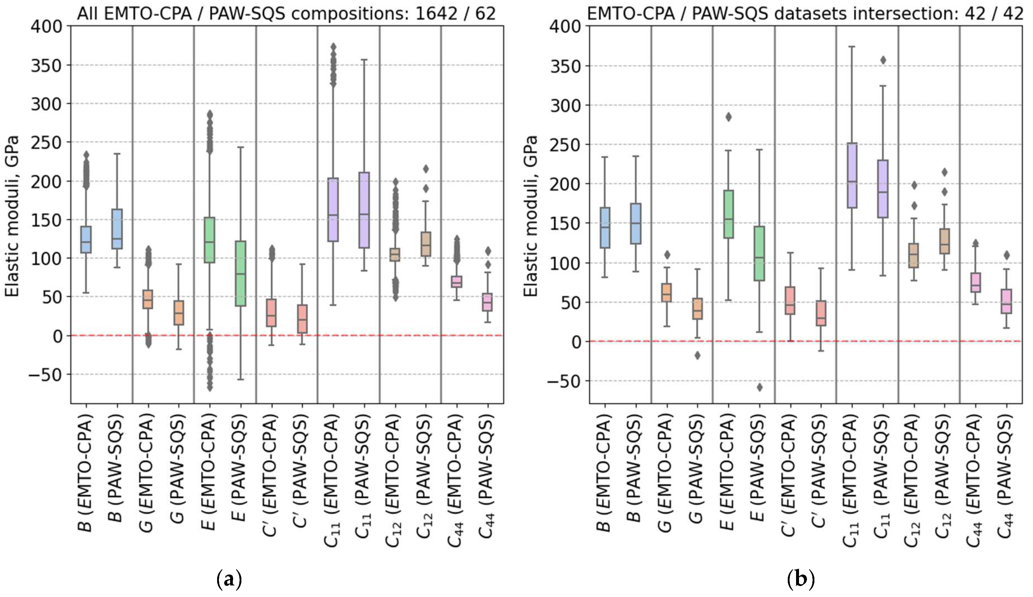
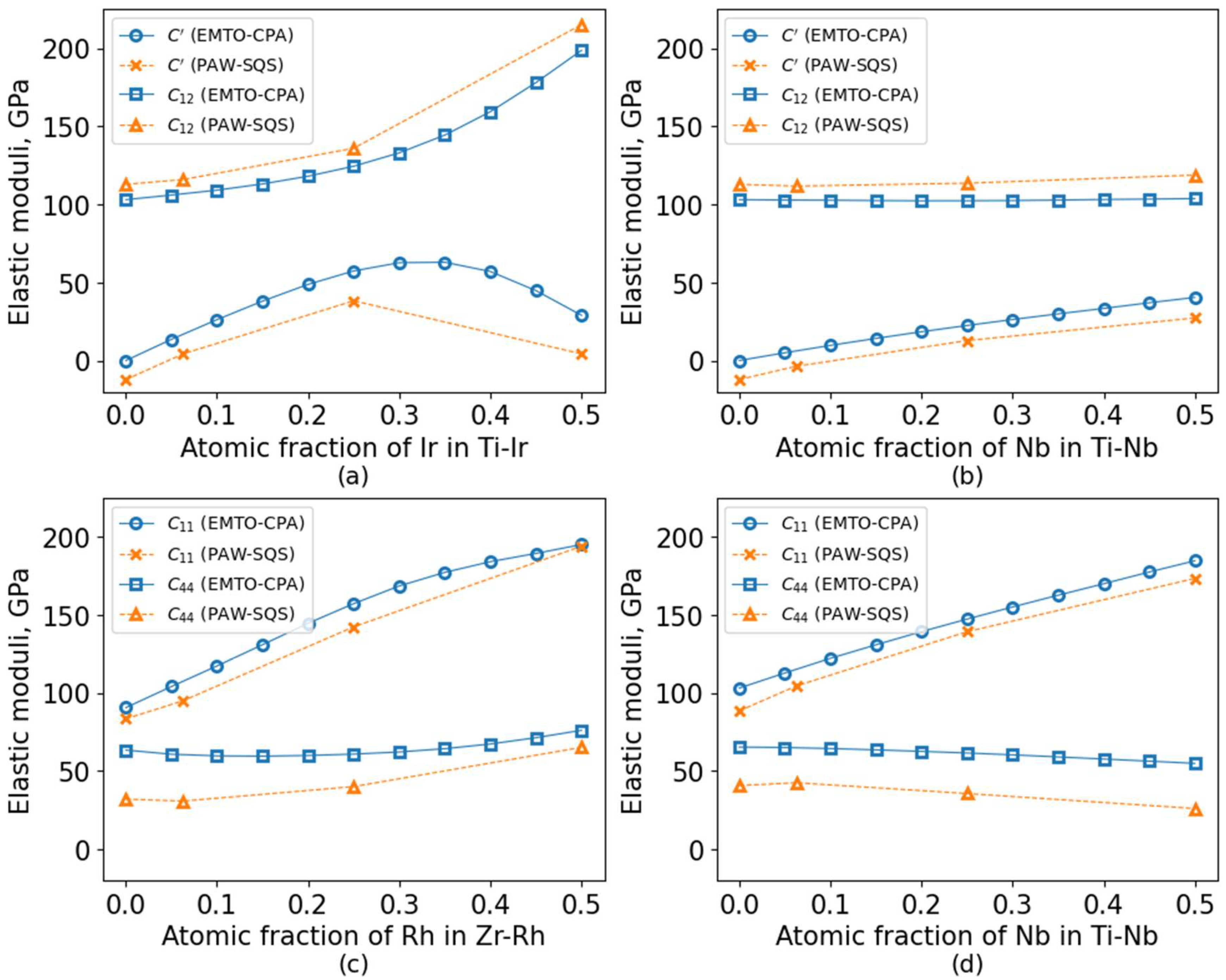
3. Results

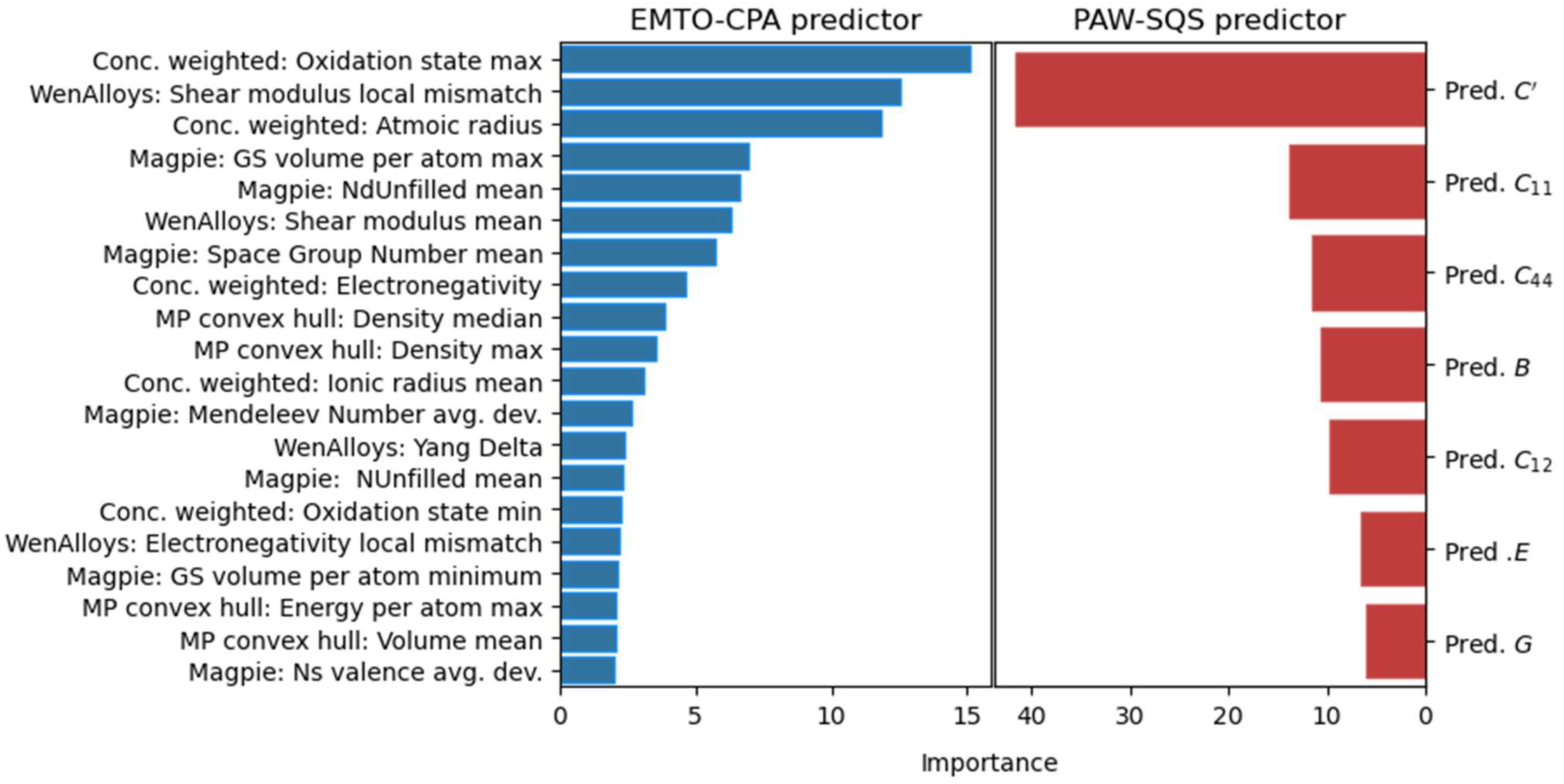
3.1. Selected Features

Feature importance analysis is shown in Figure 3. To analyze features, all feature importances, which were preserved by feature selection algorithms corresponding to the first EMTO-CPA predictor, were extracted. All selected features were represented in the following groups:

• Five features containing concentration-weighted properties of each element contained in each composition (“Conc. weighted”) with importance of 37% in total;
• Four features extracted from the “Materials Project” phase diagrams (“MP convex hull feats”) with importance of 11% in total;
• Eleven features from the “Matminer” presets (“Magpie”, “WenAlloys”) with importance of 52% in total;
• Seven features are available only for the PAW-SQS regressor predicting final values based on predictions of the first predictor (“Pred.”).

An influence of EMTO-CPA trained model predictions on PAW-SQS model predictions is shown in Figure 3.

As follows, the main contribution to the feature importance of the EMTO-CPA predictor derives from “Matminer” features, and as expected, from the concentration-weighted group. It is interesting to note that the feature importance of convex hull features that were proposed in this work confirms the assumption about their significance. All optimized model parameters are given on the GitHub page of the work.

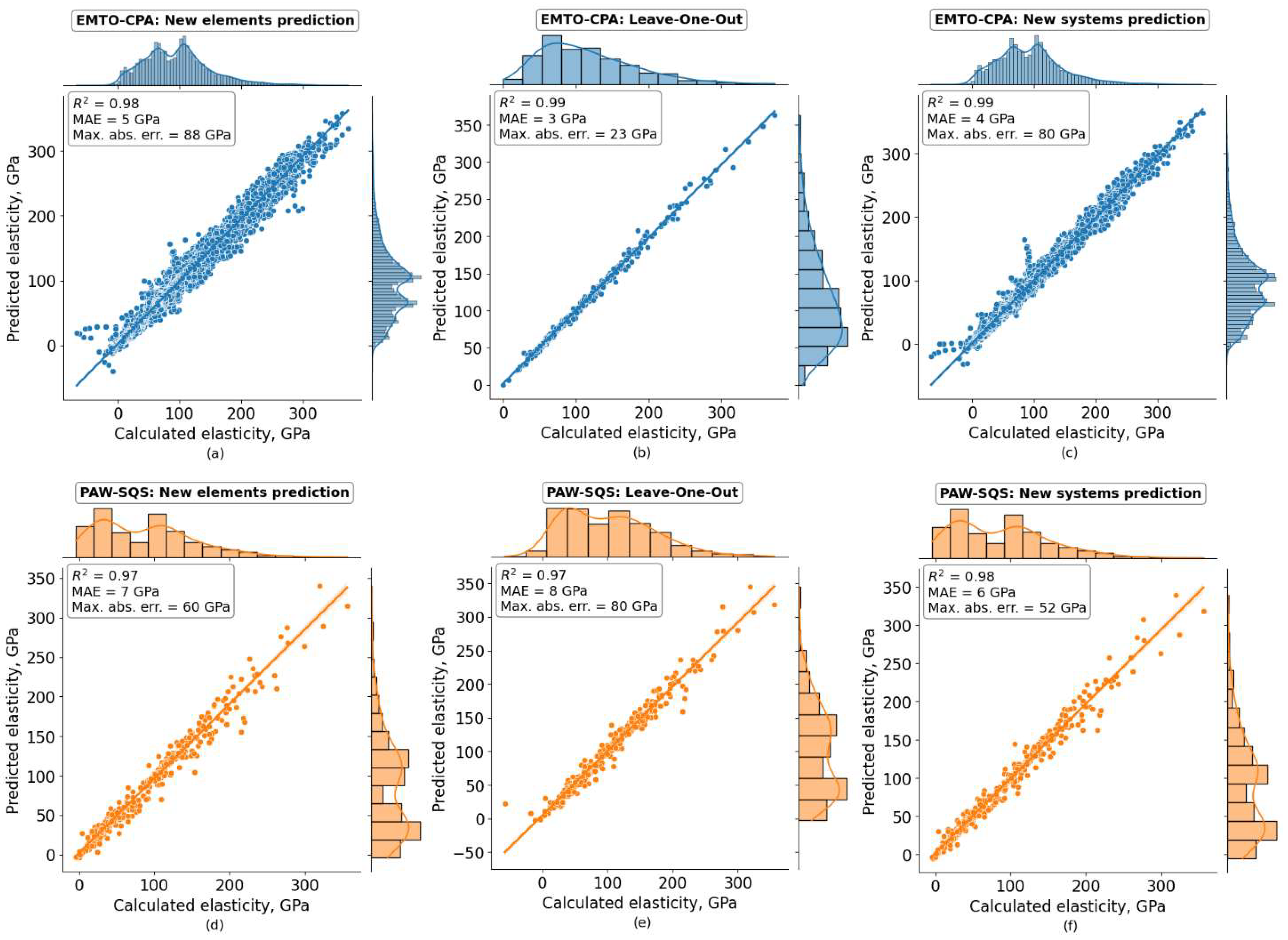
3.2. Cross-Validation Results

To assess the predictive ability of models in machine learning, data are typically randomly divided into train and test subsets step-by-step (K-fold cross-validation, K-fold CV). Thus, each defined fraction of the available data is independently included in the test dataset. However, standard CV testing does not correspond to real-use cases for datasets containing entire systems with their concentration dependencies instead of single compositions representing unique systems. Thus, for such an application, it is important, for example, to understand whether the model supplements the concentration dependencies already presented in the training set with new compositions.

In this work, cross-validation model testing in three possible use cases was performed: the prediction of properties for compositions, containing elements that were not represented in the training set (new elements prediction); the prediction of elastic properties for new concentration combinations in systems already available in the training set (leave-one-out); and the prediction of properties for systems that were not represented in the training set (new systems prediction).

In the “new elements prediction” test, compositions containing a certain alloying element from both training sets (EMTO-CPA and PAW-SQS) are sequentially excluded, which provides 34 testing folds. “Leave-one-out” testing was performed only for the intersection of two datasets, creating 42 unique folds. In the “new systems prediction” test, each chemical composition represented one of 102 test folds.

The combined results for all three types of testing (including all elastic properties E, B, G, C₁₁, C₁₂, C₄₄, and C’) are shown in Figure 4.

An assessment of overall errors demonstrates reasonable model predictions. As shown in Figure 4, the mean absolute error (MAE) of the EMTO-CPA predictor is in the range of 3–5 GPa, and the PAW-SQS predictor is in the range of 6–8 GPa. The overall result of cross-validation shows a high determination coefficient, but also high values of certain errors (max. abs. err.). Comparing the EMTO-CPA and PAW-SQS methods, it was also assumed that some deviations of the predicted values from the calculated values for the first method can be explained by the lower accuracy of the calculation of the coherent potential approximation for certain systems.

At the level of numerical data predicting, all considered elastic properties are represented with values of the same order, and a comparison of the respectively combined predicted and target values characterizes the model in general. However, it should be noted that for a more detailed description of the achieved testing metrics, prediction errors of individual properties are necessary. For example, the bulk moduli calculated within EMTO-CPA are very close to the PAW-SQS (MAE = 5.7 GPa), while for Young’s moduli, the difference is much greater (MAE = 51.2 GPa). At the same time, the concatenated data show the EMTO-CPA error in comparison with the results of the PAW-SQS calculations at the level of 21.6 GPa (MAE).

The corresponding metrics of validation tests for the separate properties are shown in

Table 1. Validation metrics.

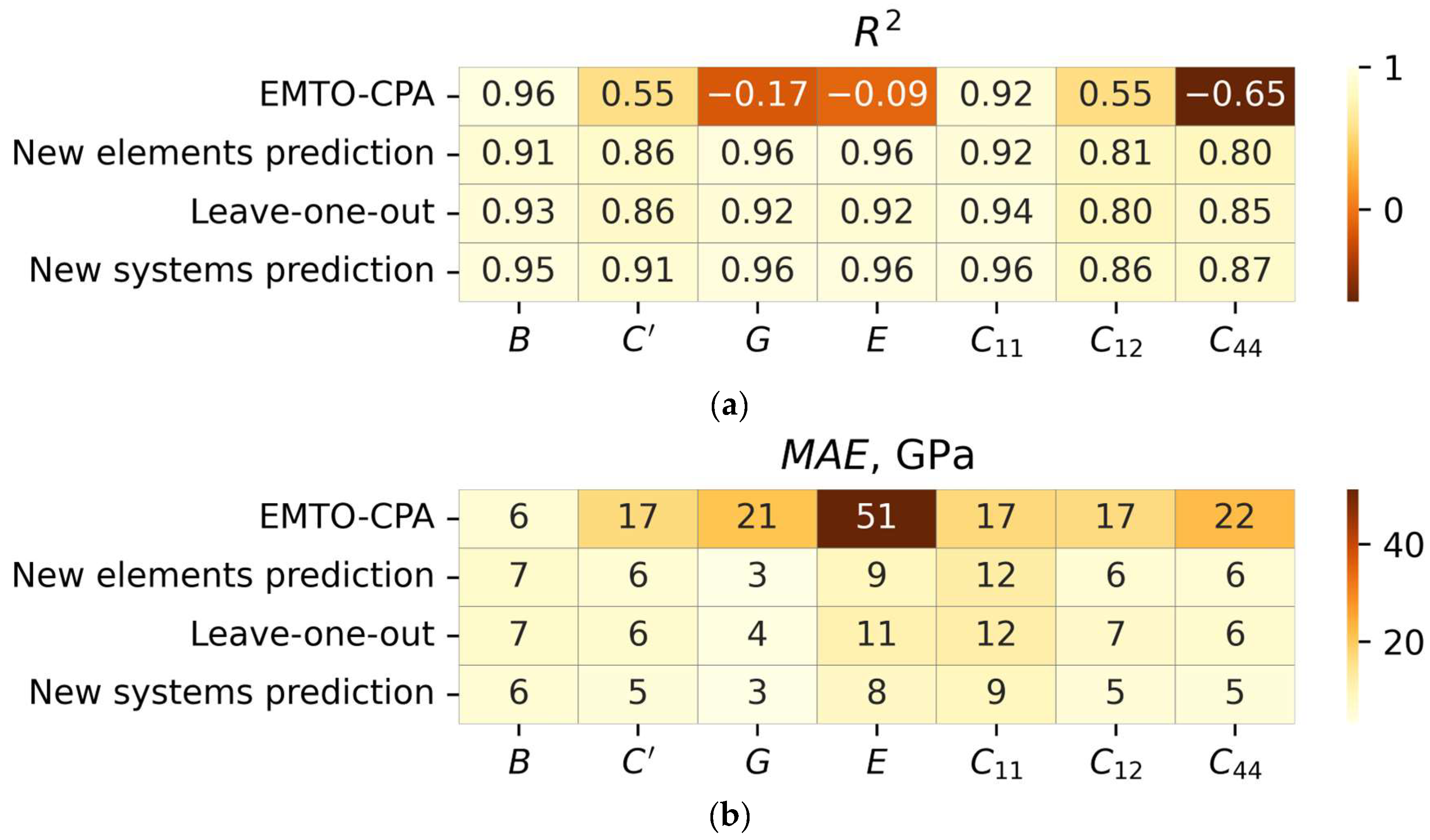
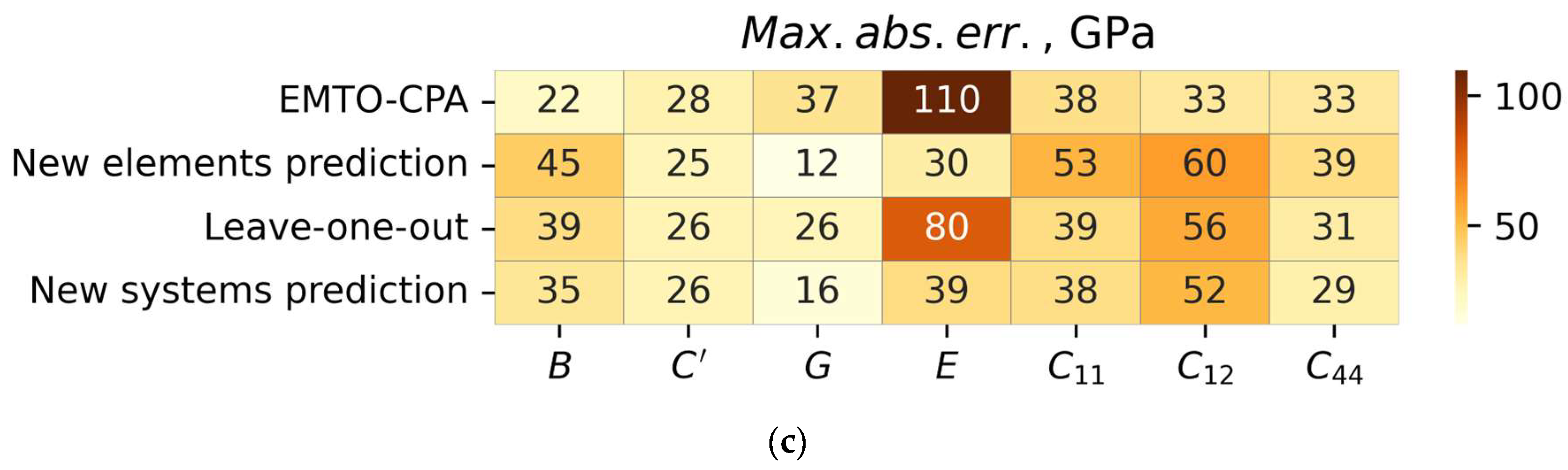
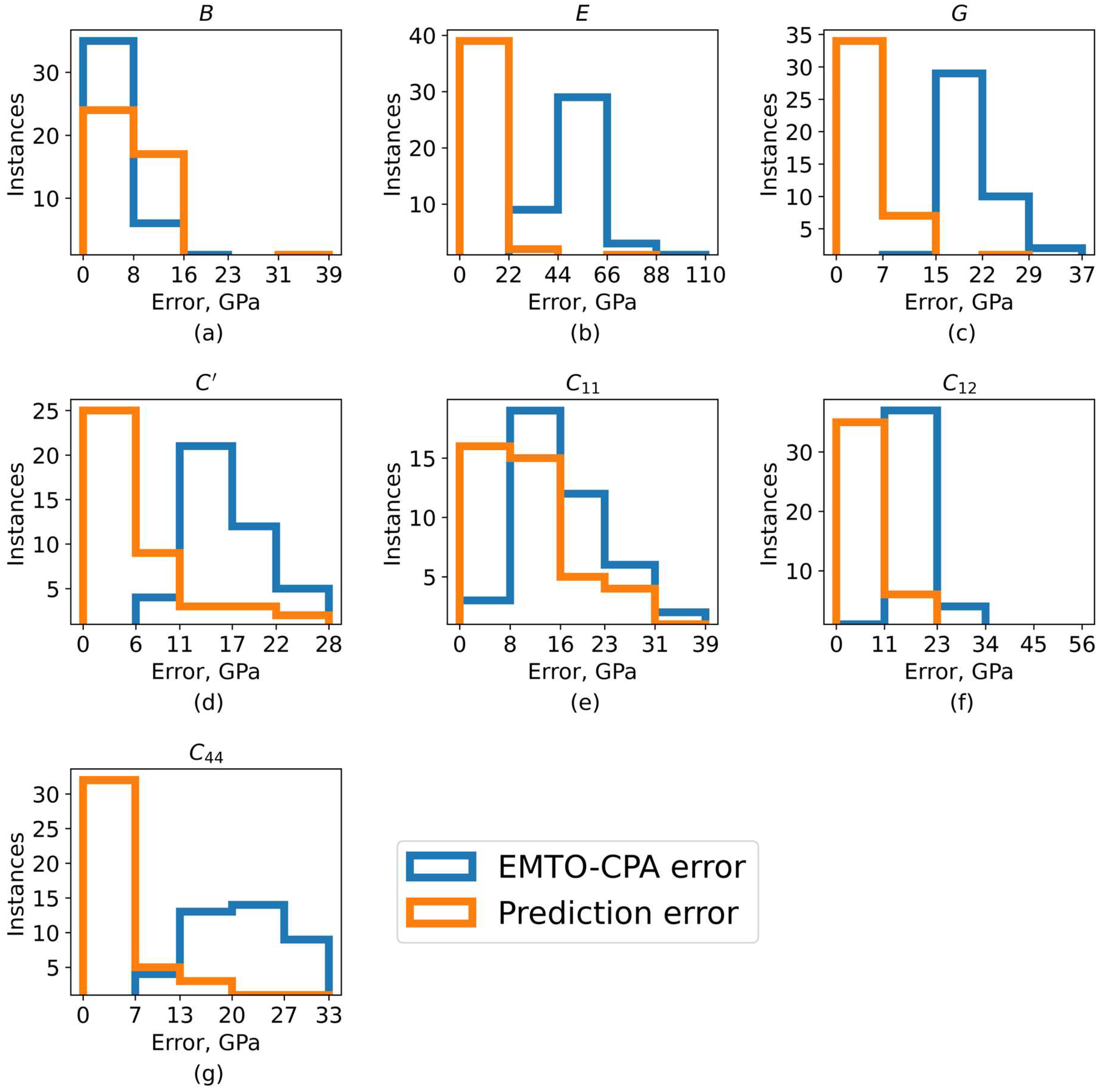
Predictor	CV Type	Property	R2	MAE, GPa	Max. Abs. Err., GPa
EMTO-CPA	New elements prediction	B	0.93	5.1	43
		C’	0.94	4.0	44
		E	0.93	8.2	86
		G	0.93	3.2	21
		C11	0.96	8.9	88
		C12	0.82	4.4	53
		C44	0.74	4.1	30
	Leave-one-out	B	0.99	3.0	11
		C’	0.98	2.8	14
		E	0.98	4.4	22
		G	0.98	1.8	9
		C11	0.99	5.5	23
		C12	0.97	2.9	16
		C44	0.97	2.2	10
	New system prediction	B	0.97	3.6	41
		C’	0.97	2.5	33
		E	0.97	5.2	53
		G	0.98	2.0	14
		C11	0.98	6.1	80
		C12	0.92	3.2	31
		C44	0.91	2.6	18
PAW-SQS	New elements prediction	B	0.91	7.2	45
		C’	0.86	6.1	25
		E	0.96	8.9	30
		G	0.96	3.4	12
		C11	0.92	12.3	53
		C12	0.81	6.1	60
		C44	0.80	6.0	39
	Leave-one-out	B	0.93	7.2	39
		C’	0.86	6.3	26
		E	0.92	10.8	80
		G	0.92	4.1	26
		C11	0.94	11.8	39
		C12	0.80	7.4	56
		C44	0.85	6.4	31
	New system prediction	B	0.95	5.7	35
		C’	0.91	4.8	26
		E	0.96	8.1	39
		G	0.96	3.1	16
		C11	0.96	9.0	38
		C12	0.86	5.2	52
		C44	0.87	5.0	29

.

The errors in the PAW-SQS correspond to the overall accuracy of the model, while based on the machine learning model-building process, it can be assumed that predictions at the level of EMTO-CPA directly influence the predictive power of the PAW-SQS predictor. This assumption is supported by the results of cross-validations. Regardless of the type of validation, both the EMTO-CPA and PAW-SQS predictors demonstrate similar general trends in MAE, showing the largest MAE in the prediction of the C₁₁ constant, and the smallest in the shear modulus (G) among other predicted properties.

The model is capable of predicting both new elements and new systems based only on the chemical composition of bcc alloys and complementing individual compositions with low levels of MAE. However, in some cases, it demonstrates rather large errors in the form of single deviations corresponding to maximum absolute errors (see Figure 4 and Table 1). To provide a general description of the contribution of these large errors to the overall distribution of prediction inaccuracies, histograms are presented in Figure 5.

To summarize Figure 5, 88% of the errors for the EMTO-CPA predictor and 79% of the errors for the PAW-SQS predictor are below 10 GPa. The most significant range of errors is between 0 and 20 GPa, since the maximum absolute error between calculations using EMTO-CPA and PAW-SQS among considered elastic properties is minimal for bulk modulus (B) and equal to 22 GPa. A quantitative assessment within this range provides an understanding of the model’s advantages over EMTO-CPA calculations.

Error distribution from Figure 5 is summarized in

Table 2. Cross-validation errors.

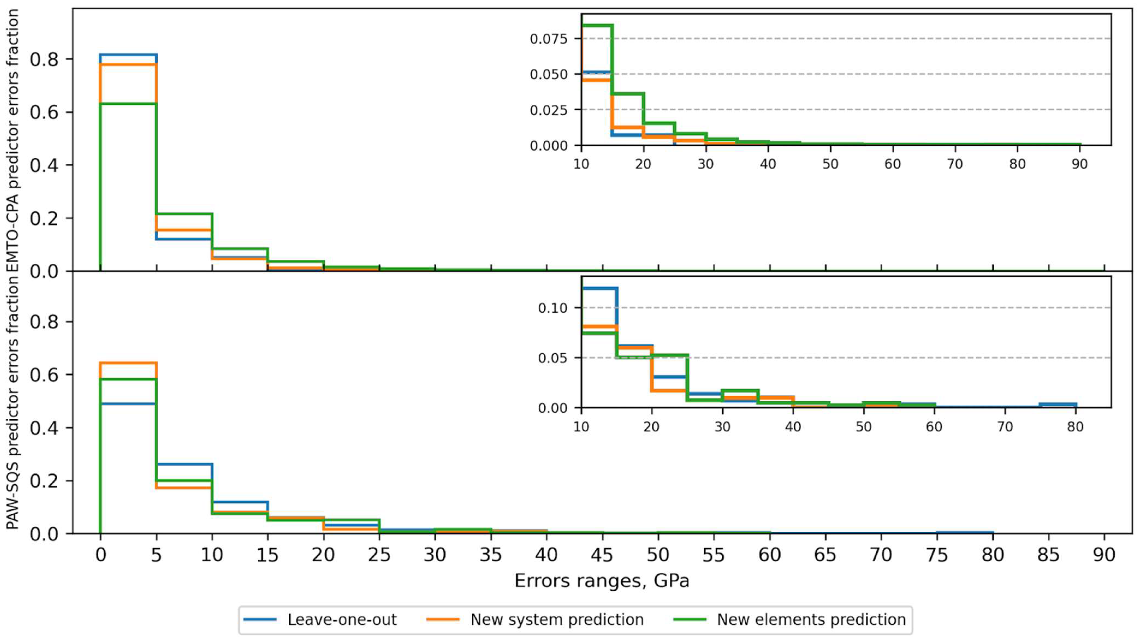
Predictor	CV Type	Errors < 5 GPa, %	Errors < 20 GPa, %
EMTO-CPA	New elements prediction	63	97
	Leave-one-out	82	99
	New system prediction	78	99
PAW-SQS	New elements prediction	58	90
	Leave-one-out	49	93
	New system prediction	64	95

for the intervals from 0 to 5 GPa and from 0 to 20 GPa.

The cross-validation error distribution demonstrates that about 70% of EMTO-CPA predictor errors and about 60% of the PAW-SQS predictor errors are between 0 and 5 GPa. Despite this, the performance of the model is assessed as sufficient because, for both predictors and validation types, more than 91% of errors are below 20 GPa. To illustrate the effectiveness of the proposed model (cross-validation results) in comparison to calculations within the EMTO-CPA framework, comparative tables of corresponding metrics for PAW-SQS calculated results are presented (Figure 6).

A comparison of all considered metrics shows that for all properties except the bulk modulus, the model outperforms EMTO-CPA calculations. The largest differences were observed for the shear (G) and Young’s moduli (E), as well as for the C₄₄ constant. The distributions of errors in EMTO-CPA calculations compared to PAW-SQS calculations and prediction errors are shown in Figure 7.

Since the PAW-SQS predictor used only the predictions of the EMTO-CPA as input features and the accuracy of the regressor used is high, it can be concluded that the PAW-SQS predictor has the potential to significantly improve the accuracy of EMTO-CPA calculations. This implies that the EMTO-CPA calculation results could be used as input for the PAW-SQS predictor directly, which could provide an additional benefit within the proposed approach.

Furthermore, a comparative analysis between the combined model and a gradient-boosting regressor trained only on the PAW-SQS dataset (reduced model) was conducted. A relevant question arises regarding the ability of a model trained only on PAW-SQS data to extrapolate to a broader test dataset beyond the original dataset, which comprises 60 compositions.

Notably, Figure 6 and Figure 7 demonstrate that the discrepancy in bulk modulus is negligible among all calculated values within the EMTO-CPA approach compared to PAW-SQS results. To evaluate the generalizability of our predictions, bulk modulus data from EMTO-CPA calculations for 1600 alloys that were not present in the intersection of the corresponding datasets as an independent validation set were used.

It is important to note that the hyperparameters and features of the reduced model were independently fine-tuned for 60 compositions and 2 pure metals for this validation test. As a result, this optimized model was directly used to predict 1600 independent data points.

In addition, to demonstrate the benefits of incorporating EMTO-CPA predictions, a 10-fold cross-validation on the combined model was performed. The results of the described tests are shown in Figure 8.

As noted above, the EMTO-CPA method demonstrates an agreement with the PAW-SQS results for bulk modulus calculation, which is shown in Figure 6, Figure 7, and Figure 8a, and observed errors exceeding 20 GPa were identified at a rate of 2% (1 out of 42 values). It has been observed that errors surpassing 20 GPa occur within a percentage of 12% (190 out of 1600 values) when using the reduced model. In contrast, errors within the corresponding range are approximately 5% (76 out of 1600 values) when utilizing a combined model.

Despite the comparable mean absolute errors of the combined model and the model trained only on the PAW-SQS dataset, the latter exhibits increased error dispersion, as evidenced by lower R² coefficients and a higher maximum absolute error. Consequently, adding the EMTO-CPA predictor to the model architecture leads to a more realistic prediction.

The effectiveness of the transfer learning principle is confirmed by testing the results of the model proposed in the work [39], where the stability of disordered face-centered cubic five-metal cation carbides was predicted using a reduced dataset. A train set of 56 samples and a test set of 7 samples was used. The less-accurate CALPHAD method calculations were used as features to improve the predictive ability of the ML model predicting the results of the more accurate PAW method. The authors show that when tested on one test set, the random forest model without additional features from CALPHAD demonstrates R² = 90.7, while adding the transfer principle leads to R² = 93.0. The predictive ability of our model can be characterized by R² values from 80 to 96 in various tests (see Table 1 and Figure 8). In another work [60], an ensemble method–random forest regressor was utilized to predict the elasticity of the ordered compounds of different symmetries based on the 1229 training samples from the materials project database. The model utilizing compositionally averaged features was tested on a 10% randomly selected hold-out set that indicated R² = 0.78 and MAE = 24 GPa for C_ij prediction. Different tests in our work demonstrated R² = 0.80–0.96, and MAE = 5–12.3 GPa for C₁₁, C₁₂ and C₄₄. In addition, for bulk modulus prediction, R² = 0.98 and MAE = 7 GPa are noted in [60]. Correspondingly, in this work R² = 0.91–0.95 and MAE = 5.7–7.2 GPa. Another work [61] shows the use of a crystal graph convolutional neural network (CGCNN) based on transferring knowledge on 8000 ordered structures represented by different structural groups to predict bulk and shear moduli of disordered alloys. The test on accurately calculated properties of relaxed disordered nitrides demonstrated MAE = 5.3–15.8 GPa for bulk modulus, whereas in this work, MAE = 5.7–7.2 GPa. In addition, the work [61] shows MAE = 7.9–23.9 GPa for shear modulus, while in this work MAE = 3.1–4.1 GPa. In general, metrics achieved by the model proposed in this work during extensive comprehensive testing are comparable to metrics shown in partially randomized tests in the literature. It can also be noted that this work proposes a model that is universal for a wide variety of doping elements of bcc-disordered alloys and is also computationally efficient enough to quickly perform large-scale predictions.

4. Conclusions

This research reveals the potential for using the computationally efficient exact muffin-tin orbital method within coherent potential approximation (EMTO-CPA) to extend the training dataset acquired through the resource-intensive projector-augmented wave method performed on special quasi-random structures (PAW-SQS) computations to build an advanced model capable of accurately predicting the elastic properties (C₁₁, C₁₂, C₄₄, C’ = (C₁₁ − C₁₂)/2, bulk modulus (B), Young’s modulus (E), and shear modulus (G)) of bcc alloys. Comparing the resource intensity of EMTO-CPA and PAW-SQS calculations for 1000 alloy compositions, the total calculation time is about 300,000 core hours for the EMTO-CPA method and about 10 million core hours for PAW-SQS.

It was demonstrated that the developed model is able to supplement the known concentration dependencies with the new compositions with high accuracy. Furthermore, a computationally efficient comprehensive approach to the development of machine learning models able to predict the properties of new bcc alloys over a wide range of concentrations and a variety of alloying elements was demonstrated.

This work further demonstrates that augmenting the training data with EMTO-CPA calculations enhances predictive ability compared to utilizing only a reduced PAW-SQS dataset. In addition, the proposed model can be used to improve the calculation results within the framework of the EMTO-CPA method.

The proposed model can be used to select promising alloys, which will then be verified by accurate calculation methods and finally be used in experimental testing. This approach reduces the time required to find the most interesting alloys for experiments, which can be expensive.

In this work, bcc-disordered alloys were considered, but it is expected that the findings of the work can be generalized for any crystal structure. The proposed method is suitable for those families of materials in which PAW-SQS calculations are time-consuming and EMTO-CPA is much more efficient, for example, high-entropy materials (carbides, oxides, borides, etc.) or Hume–Rothery alloys. Notably, it is not necessary to use two different calculation methods. The creation of both training subsets is possible within the same method, for example, only within the framework of PAW-SQS, but using different computational parameters that affect the cost of the calculation. In addition, if PAW-SQS is the only framework used, then this method can be applied to a wider class of systems.

The proposed method presumably has sufficient universality, and an accurate computational and experimental verification for other types of materials and their properties is intended to confirm the full relevance of the proposed approach. It is assumed that the prediction accuracy could be refined using an active learning framework, which would select new compositions for further calculations and add the results to the training dataset based on the greatest contribution to improve the predictive ability of the model.

References

- Biesiekierski, A.; Wang, J.; Gepreel, M.A.-H.; Wen, C. A New Look at Biomedical Ti-Based Shape Memory Alloys. Acta Biomater. 2012, 8, 1661–1669. [Google Scholar] [CrossRef]
- Mantripragada, V.P.; Lecka-Czernik, B.; Ebraheim, N.A.; Jayasuriya, A.C. An Overview of Recent Advances in Designing Orthopedic and Craniofacial Implants. J. Biomed. Mater. Res. A 2013, 101, 3349–3364. [Google Scholar] [CrossRef]
- Niinomi, M. Metals for Biomedical Devices, 2nd ed.; Woodhead Publishing: Cambridge, UK, 2019; ISBN 9780081026663. [Google Scholar]
- Li, Y.; Cui, Y.; Zhang, F.; Xu, H. Shape Memory Behavior in Ti–Zr Alloys. Scr. Mater. 2011, 64, 584–587. [Google Scholar] [CrossRef]
- Polmear, I.; StJohn, D.; Nie, J.-F.; Qian, M. Titanium Alloys. In Light Alloys; Elsevier: Amsterdam, The Netherlands, 2017; pp. 369–460. ISBN 9780080994314. [Google Scholar]
- Vitos, L. Computational Quantum Mechanics for Materials Engineers: The EMTO Method and Applications; Springer Science & Business Media: Berlin/Heidelberg, Germany, 2007; ISBN 9781846289514. [Google Scholar]
- Blöchl, P.E. Projector Augmented-Wave Method. Phys. Rev. B Condens. Matter 1994, 50, 17953–17979. [Google Scholar] [CrossRef]
- Skripnyak, N.V.; Tasnádi, F.; Simak, S.I.; Ponomareva, A.V.; Löfstrand, J.; Berastegui, P.; Jansson, U.; Abrikosov, I.A. Achieving Low Elastic Moduli of Bcc Ti–V Alloys in Vicinity of Mechanical Instability. AIP Adv. 2020, 10, 105322. [Google Scholar] [CrossRef]
- Skripnyak, N.V.; Ponomareva, A.V.; Belov, M.P.; Abrikosov, I.A. Ab Initio Calculations of Elastic Properties of Alloys with Mechanical Instability: Application to BCC Ti-V Alloys. Mater. Des. 2018, 140, 357–365. [Google Scholar] [CrossRef]
- Zunger, A.; Wei, S.; Ferreira, L.G.; Bernard, J.E. Special Quasirandom Structures. Phys. Rev. Lett. 1990, 65, 353–356. [Google Scholar] [CrossRef]
- Smirnova, E.A.; Ponomareva, A.V.; Syzdykova, A.B.; Belov, M.P. Ab Initio Systematic Description of Thermodynamic and Mechanical Properties of Binary Bcc Ti-Based Alloys. Mater. Today Commun. 2022, 31, 103583. [Google Scholar] [CrossRef]
- Hart, G.L.W.; Mueller, T.; Toher, C.; Curtarolo, S. Machine Learning for Alloys. Nat. Rev. Mater. 2021, 6, 730–755. [Google Scholar] [CrossRef]
- Wei, J.; Chu, X.; Sun, X.-Y.; Xu, K.; Deng, H.-X.; Chen, J.; Wei, Z.; Lei, M. Machine Learning in Materials Science. InfoMat 2019, 1, 338–358. [Google Scholar] [CrossRef]
- Choudhary, K.; DeCost, B.; Chen, C.; Jain, A.; Tavazza, F.; Cohn, R.; Park, C.W.; Choudhary, A.; Agrawal, A.; Billinge, S.J.L.; et al. Recent Advances and Applications of Deep Learning Methods in Materials Science. NPJ Comput. Mater. 2022, 8, 1–26. [Google Scholar] [CrossRef]
- Jain, A.; Ong, S.P.; Hautier, G.; Chen, W.; Richards, W.D.; Dacek, S.; Cholia, S.; Gunter, D.; Skinner, D.; Ceder, G.; et al. Commentary: The Materials Project: A Materials Genome Approach to Accelerating Materials Innovation. APL Mater. 2013, 1, 011002. [Google Scholar] [CrossRef]
- Haastrup, S.; Strange, M.; Pandey, M.; Deilmann, T.; Schmidt, P.S.; Hinsche, N.F.; Gjerding, M.N.; Torelli, D.; Larsen, P.M.; Riis-Jensen, A.C.; et al. The Computational 2D Materials Database: High-Throughput Modeling and Discovery of Atomically Thin Crystals. 2D Mater. 2018, 5, 042002. [Google Scholar] [CrossRef]
- Curtarolo, S.; Setyawan, W.; Wang, S.; Xue, J.; Yang, K.; Taylor, R.H.; Nelson, L.J.; Hart, G.L.W.; Sanvito, S.; Buongiorno-Nardelli, M.; et al. AFLOWLIB.ORG: A Distributed Materials Properties Repository from High-Throughput Ab Initio Calculations. Comput. Mater. Sci. 2012, 58, 227–235. [Google Scholar] [CrossRef]
- Saal, J.E.; Kirklin, S.; Aykol, M.; Meredig, B.; Wolverton, C. Materials Design and Discovery with High-Throughput Density Functional Theory: The Open Quantum Materials Database (OQMD). JOM 2013, 65, 1501–1509. [Google Scholar] [CrossRef]
- Draxl, C.; Scheffler, M. The NOMAD Laboratory: From Data Sharing to Artificial Intelligence. J. Phys. Mater. 2019, 2, 036001. [Google Scholar] [CrossRef]
- Tawfik, S.A.; Rashid, M.; Gupta, S.; Russo, S.P.; Walsh, T.R.; Venkatesh, S. Machine Learning-Based Discovery of Vibrationally Stable Materials. NPJ Comput. Mater. 2023, 9, 1–6. [Google Scholar] [CrossRef]
- Tawfik, S.A.; Russo, S.P. Naturally-Meaningful and Efficient Descriptors: Machine Learning of Material Properties Based on Robust One-Shot Ab Initio Descriptors. J. Cheminform. 2022, 14, 78. [Google Scholar] [CrossRef]
- Paz Soldan Palma, J.; Chong, X.; Wang, Y.; Shang, S.-L.; Liu, Z.-K. Thermodynamic Re-Modeling of the Yb-Sb System Aided by First-Principles Calculations. Calphad 2023, 81, 102541. [Google Scholar] [CrossRef]
- Kruthika, G.; Ravindran, P. Discerning the Crystal Structure and Engineering the Optoelectronic Properties through Substitution of Divalent Cations (M= Zn, N = Ge) in C3H3MNI3 for Solar Cell Applications. Mater. Sci. Semicond. Process. 2023, 160, 107449. [Google Scholar] [CrossRef]
- Roy, A.; Senor, D.J.; Casella, A.M.; Devanathan, R. Molecular Dynamics Simulations of Radiation Response of LiAlO2 and LiAl5O8. J. Nucl. Mater. 2023, 576, 154280. [Google Scholar] [CrossRef]
- Mukhamedov, B.O.; Karavaev, K.V.; Abrikosov, I.A. Machine Learning Prediction of Thermodynamic and Mechanical Properties of Multicomponent Fe-Cr-Based Alloys. Phys. Rev. Mater. 2021, 5, 104407. [Google Scholar] [CrossRef]
- Hayashi, G.; Suzuki, K.; Terai, T.; Fujii, H.; Ogura, M.; Sato, K. Prediction Model of Elastic Constants of BCC High-Entropy Alloys Based on First-Principles Calculations and Machine Learning Techniques. Sci. Technol. Adv. Mater. Methods 2022, 2, 381–391. [Google Scholar] [CrossRef]
- Kim, G.; Diao, H.; Lee, C.; Samaei, A.T.; Phan, T.; de Jong, M.; An, K.; Ma, D.; Liaw, P.K.; Chen, W. First-Principles and Machine Learning Predictions of Elasticity in Severely Lattice-Distorted High-Entropy Alloys with Experimental Validation. Acta Mater. 2019, 181, 124–138. [Google Scholar] [CrossRef]
- Frohlich, H.; Chapelle, O.; Scholkopf, B. Feature Selection for Support Vector Machines by Means of Genetic Algorithm. In Proceedings of the 15th IEEE International Conference on Tools with Artificial Intelligence, Sacramento, CA, USA, 5 November 2003; IEEE Computer Society: New York, NY, USA, 2004. [Google Scholar]
- Deb, K.; Pratap, A.; Agarwal, S.; Meyarivan, T. A Fast and Elitist Multiobjective Genetic Algorithm: NSGA-II. IEEE Trans. Evol. Comput. 2002, 6, 182–197. [Google Scholar] [CrossRef]
- Ward, L.; Dunn, A.; Faghaninia, A.; Zimmermann, N.E.R.; Bajaj, S.; Wang, Q.; Montoya, J.; Chen, J.; Bystrom, K.; Dylla, M.; et al. Matminer: An Open Source Toolkit for Materials Data Mining. Comput. Mater. Sci. 2018, 152, 60–69. [Google Scholar] [CrossRef]
- Xu, P.; Ji, X.; Li, M.; Lu, W. Small Data Machine Learning in Materials Science. NPJ Comput. Mater. 2023, 9, 1–15. [Google Scholar] [CrossRef]
- Ranaweera, M.; Mahmoud, Q.H. Virtual to Real-World Transfer Learning: A Systematic Review. Electronics 2021, 10, 1491. [Google Scholar] [CrossRef]
- Zhuang, F.; Qi, Z.; Duan, K.; Xi, D.; Zhu, Y.; Zhu, H.; Xiong, H.; He, Q. A Comprehensive Survey on Transfer Learning. Proc. IEEE Inst. Electr. Electron. Eng. 2021, 109, 43–76. [Google Scholar] [CrossRef]
- Lee, J.; Asahi, R. Transfer Learning for Materials Informatics Using Crystal Graph Convolutional Neural Network. Comput. Mater. Sci. 2021, 190, 110314. [Google Scholar] [CrossRef]
- Chen, H.; Shang, Z.; Lu, W.; Li, M.; Tan, F. A Property-Driven Stepwise Design Strategy for Multiple Low-Melting Alloys via Machine Learning. Adv. Eng. Mater. 2021, 23, 2100612. [Google Scholar] [CrossRef]
- Lu, T.; Li, H.; Li, M.; Wang, S.; Lu, W. Inverse Design of Hybrid Organic–Inorganic Perovskites with Suitable Bandgaps via Proactive Searching Progress. ACS Omega 2022, 7, 21583–21594. [Google Scholar] [CrossRef]
- Xin, R.; Siriwardane, E.M.D.; Song, Y.; Zhao, Y.; Louis, S.-Y.; Nasiri, A.; Hu, J. Active-Learning-Based Generative Design for the Discovery of Wide-Band-Gap Materials. J. Phys. Chem. C 2021, 125, 16118–16128. [Google Scholar] [CrossRef]
- Wanchen, Z.; Chen, Z.; Bin, X.; Xing, L.; Lu, L.; Tongxin, Y.; Yanjie, L.; Ziqiang, D.; Yi, L.; Ce, Z.; et al. Composition Refinement of 6061 Aluminum Alloy Using Active Machine Learning Model Based on Bayesian Optimization Sampling. Acta Metall. Sinica 2020, 57, 797–810. [Google Scholar]
- Kaufmann, K.; Maryanovsky, D.; Mellor, W.M.; Zhu, C.; Rosengarten, A.S.; Harrington, T.J.; Oses, C.; Toher, C.; Curtarolo, S.; Vecchio, K.S. Discovery of High-Entropy Ceramics via Machine Learning. NPJ Comput. Mater. 2020, 6, 1–9. [Google Scholar] [CrossRef]
- CatBoost—State-of-the-Art Open-Source Gradient Boosting Library with Categorical Features Support. Available online: https://catboost.ai (accessed on 20 February 2024).
- Duan, J.; Asteris, P.G.; Nguyen, H.; Bui, X.-N.; Moayedi, H. A Novel Artificial Intelligence Technique to Predict Compressive Strength of Recycled Aggregate Concrete Using ICA-XGBoost Model. Eng. Comput. 2020, 37, 3329–3346. [Google Scholar] [CrossRef]
- Ke, G.; Meng, Q.; Finley, T.; Wang, T.; Chen, W.; Ma, W.; Ye, Q.; Liu, T.-Y. LightGBM: A highly efficient gradient boosting decision tree. In Proceedings of the 31st International Conference on Neural Information Processing Systems, Long Beach, CA, USA, 4–9 December 2017; NIPS’17. pp. 3148–3157. [Google Scholar]
- Friedman, J.H. Greedy Function Approximation: A Gradient Boosting Machine. Ann. Stat. 2001, 29, 1189–1232. [Google Scholar] [CrossRef]
- Kailiang, L.; Dongping, C.; Xiaobo, J.; Minjie, L.; Wencong, L. Machine Learning Aided Discovery of the Layered Double Hydroxides with the Largest Basal Spacing for Super-Capacitors. Int. J. Electrochem. Sci. 2021, 16, 211146. [Google Scholar]
- Natekin, A.; Knoll, A. Gradient Boosting Machines, a Tutorial. Front. Neurorobot. 2013, 7, 21. [Google Scholar] [CrossRef]
- Friedman, J.H. Stochastic Gradient Boosting. Comput. Stat. Data Anal. 2002, 38, 367–378. [Google Scholar] [CrossRef]
- Vitos, L.; Abrikosov, I.A.; Johansson, B. Anisotropic Lattice Distortions in Random Alloys from First-Principles Theory. Phys. Rev. Lett. 2001, 87, 156401. [Google Scholar] [CrossRef] [PubMed]
- Kresse, G.; Joubert, D. From Ultrasoft Pseudopotentials to the Projector Augmented-Wave Method. Phys. Rev. B Condens. Matter 1999, 59, 1758. [Google Scholar] [CrossRef]
- Perdew, J.P.; Burke, K.; Ernzerhof, M. Generalized Gradient Approximation Made Simple. Phys. Rev. Lett. 1996, 77, 3865. [Google Scholar] [CrossRef] [PubMed]
- Steneteg, P.; Hellman, O.; Vekilova, O.Y.; Shulumba, N.; Tasnádi, F.; Abrikosov, I.A. Temperature Dependence of TiN Elastic Constants from ab Initio Molecular Dynamics Simulations. Phys. Rev. B Condens. Matter 2013, 87, 094114. [Google Scholar] [CrossRef]
- Hill, R. The Elastic Behaviour of a Crystalline Aggregate. Proc. Phys. Soc. A 1952, 65, 349. [Google Scholar] [CrossRef]
- Grimvall, G. Thermophysical Properties of Materials, 1st ed.; Elsevier Science: Amsterdam, The Netherlands, 1999; Enlarged and revised edition; p. 52. ISBN 0444827943. [Google Scholar]
- Mouhat, F.; Coudert, F.-X. Necessary and Sufficient Elastic Stability Conditions in Various Crystal Systems. Phys. Rev. B Condens. Matter 2014, 90, 224104. [Google Scholar] [CrossRef]
- Ong, S.P.; Richards, W.D.; Jain, A.; Hautier, G.; Kocher, M.; Cholia, S.; Gunter, D.; Chevrier, V.L.; Persson, K.A.; Ceder, G. Python Materials Genomics (pymatgen): A Robust, Open-Source Python Library for Materials Analysis. Comput. Mater. Sci. 2013, 68, 314–319. [Google Scholar] [CrossRef]
- Ward, L.; Agrawal, A.; Choudhary, A.; Wolverton, C. A General-Purpose Machine Learning Framework for Predicting Properties of Inorganic Materials. NPJ Comput. Mater. 2016, 2, 16028. [Google Scholar] [CrossRef]
- Wen, C.; Zhang, Y.; Wang, C.; Xue, D.; Bai, Y.; Antonov, S.; Dai, L.; Lookman, T.; Su, Y. Machine Learning Assisted Design of High Entropy Alloys with Desired Property. Acta Mater. 2019, 170, 109–117. [Google Scholar] [CrossRef]
- Zhang, R.F.; Zhang, S.H.; He, Z.J.; Jing, J.; Sheng, S.H. Miedema Calculator: A Thermodynamic Platform for Predicting Formation Enthalpies of Alloys within Framework of Miedema’s Theory. Comput. Phys. Commun. 2016, 209, 58–69. [Google Scholar] [CrossRef]
- Schmidt, J.; Pettersson, L.; Verdozzi, C.; Botti, S.; Marques, M.A.L. Crystal Graph Attention Networks for the Prediction of Stable Materials. Sci. Adv. 2021, 7, 7948. [Google Scholar] [CrossRef] [PubMed]
- Prokhorenkova, L.; Gusev, G.; Vorobev, A.; Dorogush, A.V.; Gulin, A. CatBoost: Unbiased boosting with categorical features. In Proceedings of the 32nd International Conference on Neural Information Processing Systems (NIPS’18), Montréal, QB, Canada, 3–8 December 2018; Curran Associates Inc.: Red Hook, NY, USA, 2018; pp. 6639–6649. Available online: https://dl.acm.org/doi/10.5555/3327757.3327770 (accessed on 16 February 2024).
- Rajan, K. Machine Learning Elastic Constants of Multi-Component Alloys. Comput. Mater. Sci. 2021, 198, 110671. [Google Scholar]
- Levämäki, H.; Tasnádi, F.; Sangiovanni, D.G.; Johnson, L.J.S.; Armiento, R.; Abrikosov, I.A. Predicting Elastic Properties of Hard-Coating Alloys Using Ab-Initio and Machine Learning Methods. NPJ Comput. Mater. 2022, 8, 2–10. [Google Scholar] [CrossRef]