Simulation Models in a Fluidity Test of the Al-Si Alloy

Abstract

The goal of the fluidity test is to evaluate the ability of the melt to fill the cavity of the mold, which is one of the factors affecting the final quality of the castings. It is a technological test that is basically not standardized, therefore it is realized in different forms, for example using “horizontal” and “vertical” molds. The “horizontal” mold makes it easier to fulfill the condition of repeatability, therefore it was used to calculate the capability of the test by the Measurement Systems Analysis (MSA) method. The results of the tests in both molds were used to calculate regression equations that allow the fluidity to be determined with strong reliability based on variables such as melt temperature, casting speed, and mold temperature. In addition, the effects of input data variability (uncertainty) on the resulting fluidity value were analyzed using regression equations and the Monte Carlo simulation. The contribution of the article is the analysis of the capability of the measurement process of the fluidity and a prediction of the results of its tests using the Monte Carlo simulation method.

1. Introduction

In the context of ensuring the metrological quality assurance of products, it is crucial to monitor all measurement processes involved in their development, production, commissioning, and maintenance. A measurement process encompasses a series of related resources, operations, and factors that result in a measurement outcome. This process should be treated like any other process requiring management. It initiates by linking the measuring devices to the standard values, followed by metrological confirmation, and culminates in the actual measurement conducted by specific individuals, all while considering various influencing factors. The management of measurement processes is based on the routine monitoring and analysis of measurement data, as highlighted in the references [1,2].

The EN ISO 9000 standard [3,4] describes quality as how well a set of inherent characteristics meets requirements. In this context, the quality—the capability of the being analyzed—is assessed based on the statistical properties of a large number of measurements from a measurement system under stable conditions [5]. If a measurement system exhibits high variability, it may be inadequate for process analysis because the system’s variability could obscure the process’s own variability [6,7].

The measurement process occurs within a specific system that includes, at a minimum, the measuring device, the methodology, the operator (the objects being measured (parts, samples)), and the surrounding environmental conditions. Evaluating the capability of the measurement system provides a practical assessment and measure of the quality of the measurement process implemented. Adopting relevant standards, such as ISO 9000, ISO 10012 [8], and ISO/IEC 17025, significantly enhances the measurement process’s quality [9,10].

The fluidity test stands out as a critical assessment in foundry operations, where fluidity refers to the capacity of molten metal to completely fill a mold cavity and accurately replicate its shape. However, due to the lack of established standards for measuring fluidity, assessing the effectiveness of the process through uncertainty analyses remains challenging.

According to ISO 10017:2021 [11], simulation encompasses a range of techniques in which a system is digitally modeled using computer software to address a specific question. This approach is particularly valuable in theoretical science, where it serves as a tool in the absence of a comprehensive theoretical framework for problem solving, or where direct solutions are impractically expensive or computationally demanding. Specifically, the Monte Carlo method, a form of simulation, is used when direct computation of problem solutions is either not feasible or too resource intensive.

Fluidity is determined by pouring molten metal into a standardized mold to produce a thin, elongated casting, typically in the form of a spiral or rod. The length of this spiral or rod is then used as an indicator of the fluidity of the metal [12,13].

Unlike physical properties such as surface tension or liquidity, which describe the state of the liquid metal, fluidity is a technological property that is influenced by a number of factors that affect how the mold is filled. Key factors include the following [7,14]:

• Alloy properties, including viscosity, surface tension, density, and thermal conductivity.
• The metal’s temperature at the time of casting.
• The design of the inlet system through which the metal enters the mold.
• Mold properties, such as thermal conductivity, density, and the coefficient of friction between the melted metal and the mold walls.
• The configuration of the casting as it solidifies.
• Environmental conditions, including ambient temperature, pressure, and geoclimatic factors.

Various technological tests are used to assess fluidity, of which only the fluidity test for cast steel is standardized [15].

It is important to note that the results of these tests can only be reliably compared if they are performed under identical conditions, using the same molds and casting techniques. Small variations in casting temperature can have a significant effect on the results, often outweighing the impact of other factors. For a fluidity test to be considered effective, it must be both sensitive and reproducible. The Measurement Systems Analysis (MSA) provides insights into the capability of the fluidity test by evaluating its precision [6,16].

In addition, alternative test methods such as variable cross-section tests (e.g., V-belts or the Spassky ball point test) are used to measure the capacity of the melt to fill very fine sections. These tests are particularly valuable for alloys that tend to form an oxidation layer on the surface [12,15,17].

Aluminum alloys with a silicon content of between 7 and 18 wt.% exhibit superior fluidity. However, the presence of iron has a contrasting effect. Wang [18] highlighted the impact of iron on brazing processes, in particular the problem of adhesion between the iron mold and the aluminum casting. As the article uses iron molds for device testing, monitoring the iron content becomes critical. Iron in concentrations of 0.3 wt.% to 0.5 wt.%, can reduce sticking and improve the casting’s strength, hardness, fluidity, and mechanical properties at elevated temperatures. Conversely, iron levels above 0.5 wt.% lead to the formation of brittle FeSiAl₅ (β phase) needles. These needles, when penetrating the aluminum matrix and eutectic cells, increase the risk of premature casting failure due to notching caused at higher iron concentrations.

The fluidity test, a key technological assessment, is conducted using different methods tailored to specific conditions such as the alloys used, temperature, and casting requirements. The authors selected two fluidity measurement methods and analyzed them through the lens of the MSA quality. The data collected were used to develop regression equations, providing a method for estimating fluidity without the need for costly practical experiments that consume significant material, time, and energy. Simulations were carried out to ensure the sustainability of the research, taking into account its considerable time and energy requirements. In addition, the regression equation facilitates the prediction of production quality, for example using the Monte Carlo method mentioned above. This predictive capability is crucial for sustaining research activities in the future, as it helps to avoid activities that significantly inflate research costs.

The aim of this study is to determine the relationships between the values of fluidity obtained by experimental tests in the “horizontal” three-channel mold, designed according to the method of measurement systems analysis (MSA) [6]. The mold’s design is particularly effective for assessing the measurement process’s capability to accurately measure fluidity, primarily by facilitating tests under repeatable conditions. The MSA approach is endorsed in automotive reference manuals and supports compliance with the IATF ISO/TS 16949:2016 standards [19].

2. Materials and Methods

The main objective of the experiment was to determine the influence of various factors (operator—the founder, the temperature of the melted alloy, pouring velocity/casting speed, and the temperature of mold pre-heating) on flow behavior with a “vertical” and “horizontal” mold.

The alloy AlSi10 (DIN 1725) with 10.54% of silicon was used as the test material. Iron (up to 0.15%) was the polluting element. The charge was melted in a chamotte–graphite crucible in an electric resistance furnace.

The reported casting temperatures, their expanded uncertainties U_c, pouring velocities, and the actual temperature of the ready-to-cast molds for the two operators (A, B) who carried out the casting and both the molds are given in

Table 1. The selected pouring temperature, its combined extended uncertainty, pouring velocity, and temperature of the molds for both operators (A, B) and both molds.

Temperature of the melt (°C)		operator	600	650	670	680	700	720	750	760	780	830
Uncertainty Uc (°C)		A	3.00	3.00	3.13	2.93	3.00	3.43	3.09	3.31	3.31	3.11
		B	3.14	3.02	3.43	2.94	3.54	3.29	4.17	3.09	3.25	3.11
Pouring velocity (g s−1)	“horizontal” mold	A	102	93	93	98	101	101	91	93	99	98
		B	111	98	98	123	108	96	92	121	109	108
	“vertical” mold	A	89	91	91	98	90	96	91	93	99	98
		B	111	121	121	123	129	96	92	121	131	108
Temperature of the mold (°C)	“horizontal” mold	A	121	122	121	118	118	120	120	122	125	129
		B	111	122	121	118	121	118	118	120	120	129
	“vertical” mold	A	120	120	112	121	120	120	120	122	125	129
		B	112	122	121	125	127	130	130	129	128	129

. The pouring velocity given in the article is an average value, i.e., the ratio between the weight of the melt poured into the mold and the time of pouring. The Grubbs test was used (two-sided with a significance level of α = 0.05). No outliers were found for pouring velocity or mold preheating.

The temperature of the molten alloy was measured three times with a chromel–alumel (K) submerged thermocouple in a protective ceramic housing using a calibrated TESTO term 9010 digital meter. When the set point specified in the first row of Table 1 was reached, the crucible with the melt was removed from the furnace. The surface of the melt was cleaned from the oxidized layer (dross). Cleaning was carried out mechanically with a rake until a clean surface was achieved. This cleaning did not affect the temperature of the molten alloy. Additives such as eutectic silicon modifiers, grain refiners, and degassing salts were not used. The treated molten alloy was then poured into the “horizontal” mold and after, into the “vertical” mold. The temperature drop of the melt was negligible when poured into both molds.

To calculate the uncertainty of the melt temperature, it was measured three times at a temperature close to the intended casting temperature. The combined uncertainty of the melt temperature U_c shown in Table 1 was calculated according to Equation (1) from the results of the calibration (standard uncertainty u_B) and the standard deviation (SD) of the repeated temperature measurements (standard uncertainty u_A), with the coverage factor k = 2.

$$U_c=k·\sqrt{u_A^2+u_B^2}$$

(1)

The “horizontal” mold made it possible to calculate the capacity of the flow test in relative terms. The three-channel system, described below, allows conditions for repeatability to be created for the measurement system analysis (MSA) [6]. This arrangement allows the number of tests to be reduced. The results, supplemented by a computer simulation (software Novaflow&Solid Version 6.5) have been published in [20,21].

Theoretically, this is also possible with a “vertical” mold; however, it requires more time-consuming tests. Further research will also focus on this direction.

The “horizontal” bar-type three-channel mold (Figure 1 and Figure 2, mold marked as A) was designed as a demountable mold with parts screwed together. The steel core (channels and bottom) was connected to an aluminum alloy base plate to avoid possible distortion. The steel mold, with a height of 255 mm and a channel diameter of 20 mm, was used as a sprue. The height of all three “horizontal” channels was 10 mm and the width was 5 mm (the cross-section was 50 mm²). The melt was poured into the square area—the gate below the sprue eliminates the negative effects of sharp angles. The mold was preheated to 120 °C ± 10 °C before casting. Once the casting had solidified and the screws had been loosened, the casting was released. The temperature of the mold was measured with thermocouples at four points. Table 1 shows the average temperatures of these four points just before the melt was poured into the mold. The value of fluidity L [mm] is the average distance of the melt flow in all three channels.

The “vertical” mold with the cavity in the shape of a harp (or lyre) was used for the multi-bar “vertical” test, (Figure 2, mold marked B). It was milled from a solid block of steel. It was also preheated to 120 ± 10 °C before casting. The temperature of the mold was measured at two points with a thermocouple. Table 1 shows the average temperatures at these two points just before the molten metal was poured into the mold. The mold had a row of 6 bars (risers, vertical channels) with diameters D₁ = 4.5 mm, D₂ = 6.5 mm, D₃ = 8.5 mm, D₄ = 10.5 mm, D₅ = 12 mm, and D₆ = 14 mm.

The value (coefficient) of the fluidity [mm] is calculated by Equation (2).

$$Y_z=\frac{S_1}{L_1}+\frac{S_2}{L_2}+\frac{S_3}{L_3}+\frac{S_4}{L_4}+\frac{S_5}{L_5}+\frac{S_6}{L_6}$$

(2)

L is the height of the alloy column in the bar/riser [mm], and S is the cross-section of the given bar [mm²].

The pouring velocity/casting speed (g.s⁻¹) was measured by placing the molds on a scale and recording the weight gain as a function of time. The average value was taken into account.

The casting process was carried out by two operators (A, B), both with the same skill and experience. The selected pouring temperature and the order of the operators were determined randomly (by drawing lots). The values of fluidity coefficients are given in

Table 2. Values of fluidity coefficients L for “horizontal” and Yz for “vertical” molds.

Operators	T (°C)	600	650	670	680	700	720	750	760	780	830
A	L (mm)	25.2	47.3	54.7	93.1	73.0	147.0	152.7	155.3	165.0	174.7
	Yz (mm)	3.4	4.52	3.78	6.08	5.87	9.09	9.92	9.92	10.56	10.65
B	L (mm)	44.5	76.0	75.3	77.0	112.0	93.7	130.0	145.7	131.3	258.0
	Yz (mm)	3.96	6.42	6.37	7.15	10.39	8.79	9.99	9.99	10.95	6.62

.

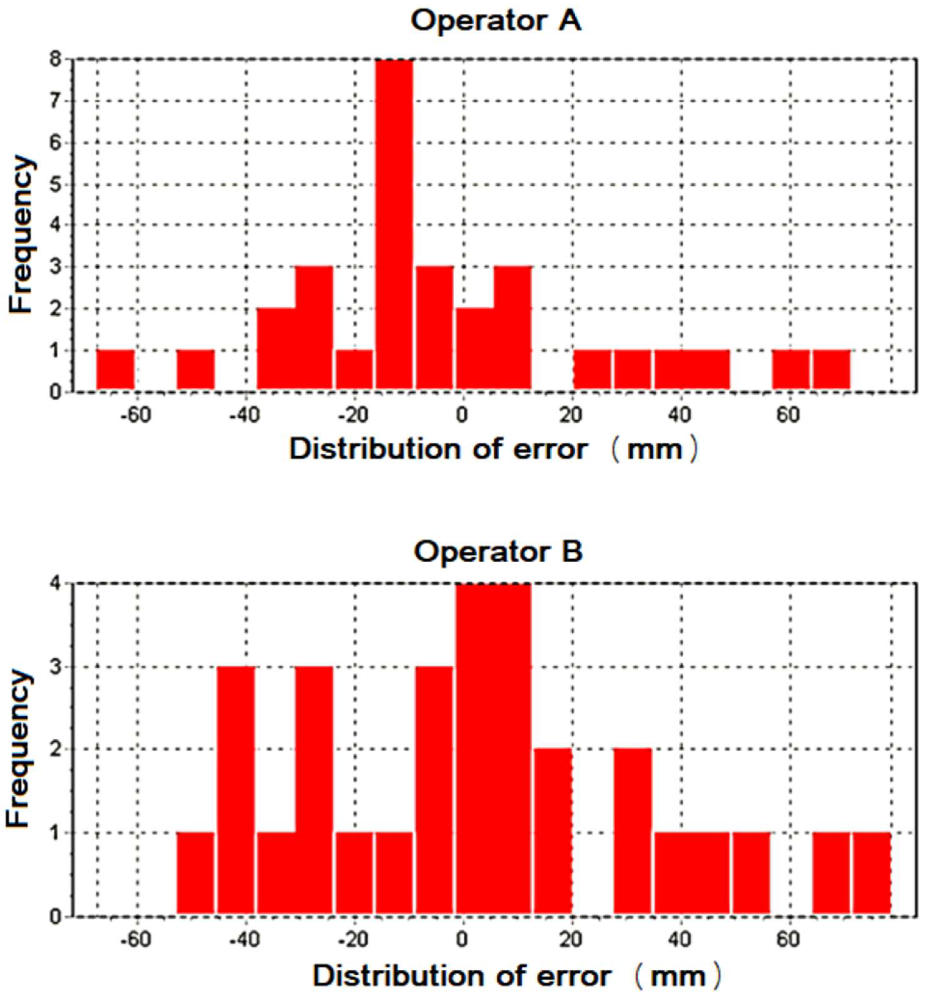
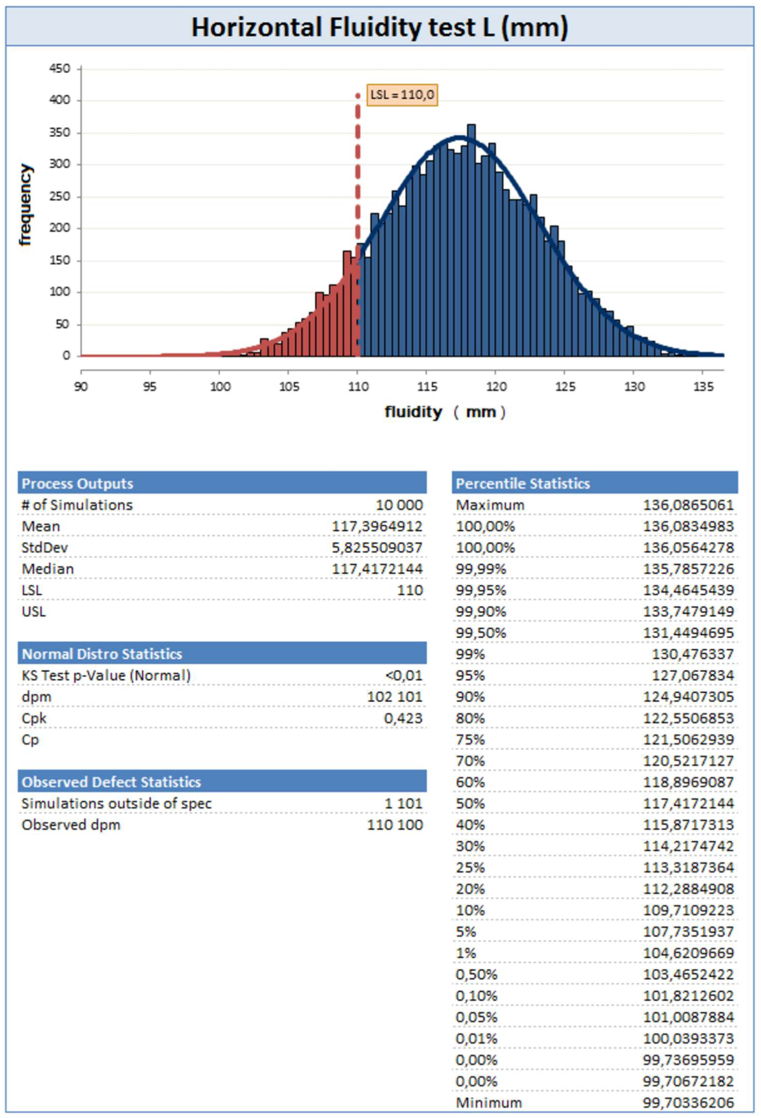
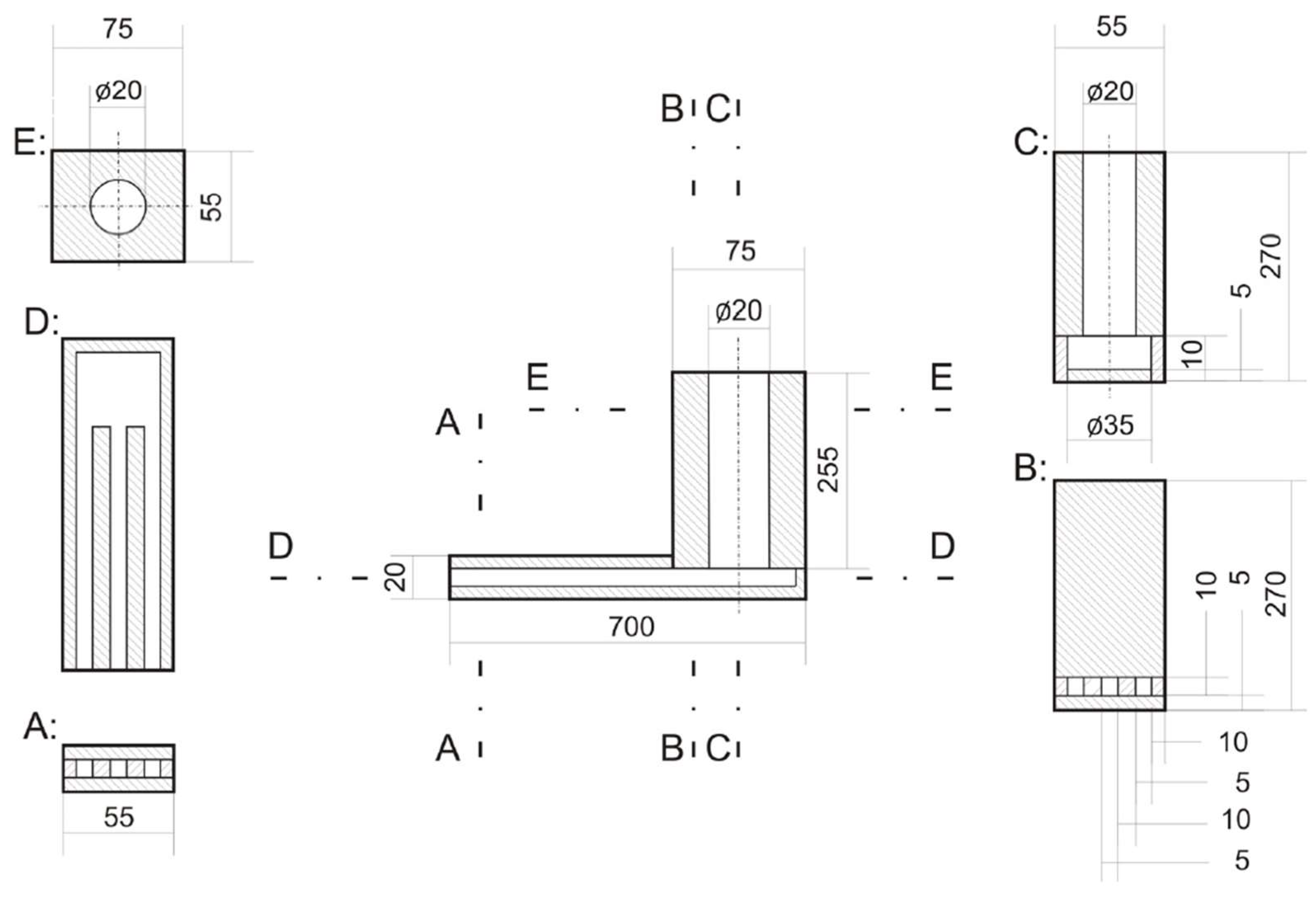
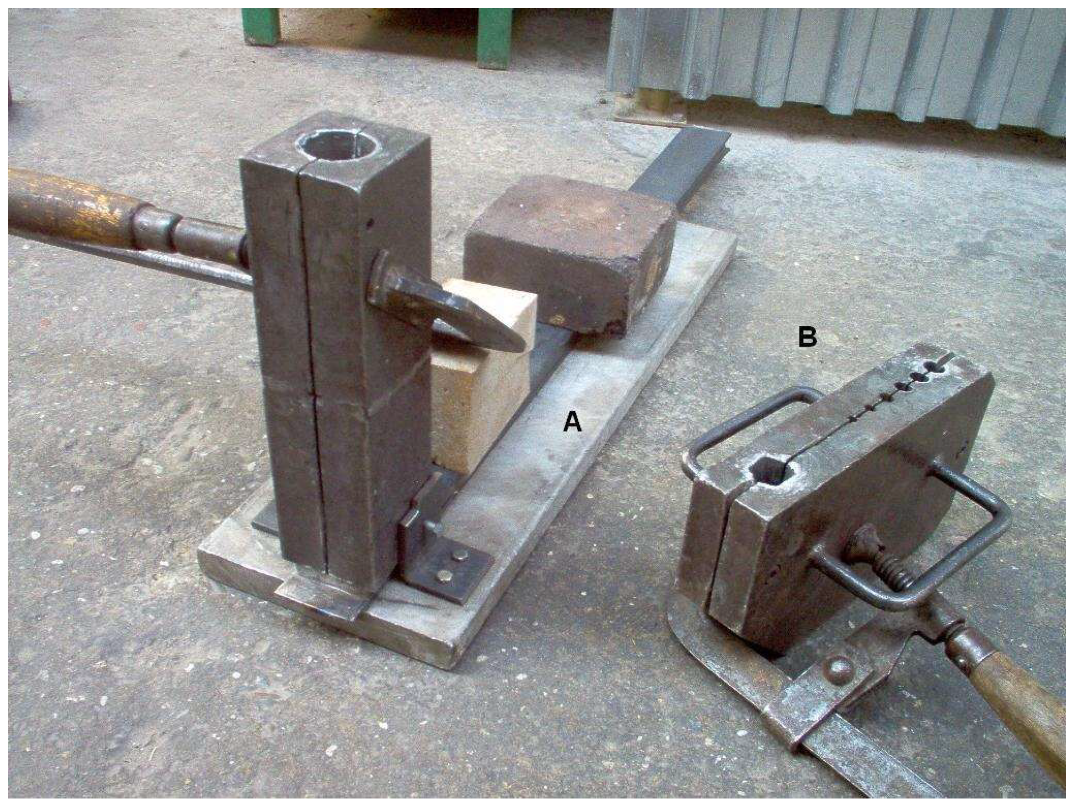
The Evaluation of the Capability of Measurement by the “Horizontal” Mold

The capability of the Al-Si fluidity test in a “horizontal” form was estimated by a measurement systems analysis (MSA) [4]. The experiment was performed with 2 operators, 10 levels of pouring temperature (10 “parts”), and 3 trials (length of flow in each channel).

A measuring device with a sufficient resolution should be selected for the measurement. As a general rule, it should be able to subtract at least one-tenth of the expected variability of the character being tested. The height of the metal penetration in the rods was measured with a caliper with an accuracy of 0.1 mm.

The standard deviation (SD) of all the fluidities measured (three channels, 10 temperature levels, two operators) was 60.63 mm, and the condition of sufficient resolution of the measuring device was fulfilled.

Outlier fluidity values were determined using the Grubbs test at a significance level of α = 0.05% and were not detected. Normality was determined by using the Anderson–Darling test. The values measured by operator A had a normal distribution (p = 0.292384), but the values measured by operator B had an irregular distribution (p = 0.00426). A normal distribution requires standard methods for analyzing measurement systems. If the system does not have a normal distribution, the MSA method can overestimate the system error. This means that a capability is presented that is worse than it is.

The analysis of the capability of the measurement system is not yet standardized. The absence of a standard is currently covered by company standards, which are mainly used in the automotive industry. The Measurement Systems Analysis (MSA) manual was developed on the basis of these standards. The manual is a supplementary document to the standard (technical specification) STN ISO/TS 16 949:2002 [22]. The following applies: if the measurement process is implemented in a qualified system that includes operators, measuring equipment, environmental conditions, parts, etc., it is assumed that the process itself is also capable. The measurement system can be analyzed based on the determination of repeatability and reproducibility (mean and range methods—GRR) or using an analysis of variance (ANOVA). An analysis of variance allows more information to be obtained from experimental data but requires more complex calculations and a certain degree of statistical knowledge to interpret the results [6].

The GRR method used Is a combined estimate of the repeatability and reproducibility of the measurement system at a significance level of 99% with a coverage interval of 99% (5.15 α). It enables the variability to be broken down into two separate components, but, unlike ANOVA, does not express their interaction. Software from Palstat (https://www.palstat.cz/en/ (11 December 2023)), p.r.o. was used for routine calculations.

The number of parts or samples (the number of samples corresponds to the number of selected pouring temperatures, i.e., 10) and repeated measurements (in our case, this was the repeated measurement of the melt flow in each channel during casting by one operator at the selected pouring temperature, i.e., the number of repetitions (n = 3)) depends on the importance of the measured characteristic and the confidence level (significance level) required to estimate the variability of the measurement system. As with most statistical methods, the larger the sample size, the smaller the variability of the selection and the lower the resulting risk.

Among the MSA options, the repeatability and reproducibility analysis GRR was used next.

The first step in evaluating the GRR is to assess whether the measurement process is statistically controlled in terms of the variability of repeated measurements made by individual operators. For this evaluation, it is necessary to create a control chart for the values of the range of variation (the difference between the maximum and minimum value of the melt flow in the channel). The level of the central line of the control chart corresponds to the average variation range for all casting temperatures and operators.

The control chart of the variation range (Figure 3) shows that the measurement process is not statistically controlled with respect to the variability of the repeated measurements, since all values of the variation range are within the control lines, which are a function of the average range of the measured values and coefficients depending on the number of measurement repetitions. After the statistical control of the process, the repeatability is calculated (EV—Equipment Variation, Repeatability) by Equation (3):

$$EV=5.15\ast \frac{\stackrel{̿}{R}}{d_2^{*}}$$

(3)

The coefficient d₂^* in Equation (3) depends on the number of measurement repetitions (3), the levels of pouring temperature (10), and the number of operators (2). The multiple of the standard deviation 5.15 σ corresponds to the width of the range in which 99% of all values lie, assuming a normal distribution of the measured characteristic.

The next procedure focuses on the evaluation of the reproducibility of the measurement, which characterizes the variability between the operators. In the first approach, the values of the arithmetic diameters of the currents determined by the individual operators are determined. Based on the specified variation, range value (4) can be calculated as the reproducibility (AV—operator variation) of the measurement (5):

$$R_0={\overline{x}}_{i max}-{\overline{x}}_{i min}$$

(4)

$$AV=\sqrt{{(5.15\ast \frac{R_0}{d_2^{*}})}^2-\frac{{EV}^2}{n\ast r}}$$

(5)

r = the number of levels of the pouring temperature (10), n = the number of repeated measurements (”flows” of the melt in three channels—3), and d₂^* in Equation (5) depends on the number of operators (2).

The repeatability and reproducibility are calculated by Equation (6):

$$GRR=\sqrt{{EV}^2+{AV}^2}$$

(6)

The variation range of the arithmetic diameter of “flow” of the melt at individual casting temperature levels is determined by Equation (7):

$$R_p={\overline{x}}_{\max j}-{\overline{x}}_{\min j}$$

(7)

Equation (8) applies to the determination of the variability between individual casting temperatures—the part variability (PV):

$$PV=5.15\ast \frac{R_p}{d_2^{*}}$$

(8)

Index d₂^* in Equation (8) depends on the number of pouring temperature levels (10).

The suitability of the measuring system for assessing the variation between runs at each temperature level can be assessed using the diameter control chart (X—bar control chart), seen in Figure 4. The central line of the control chart corresponds to the arithmetic mean of all measured values of the runs.

The system is considered suitable for evaluating the variability of the casting temperatures when most of the ranges lie outside of the control lines. In the system tested, 65% of the elevated values were between the control limits.

The total variability of TV measurement (Total Variation) is applied by Equation (9):

$$TV=\sqrt{{EV}^2+{AV}^2+{PV}^2}$$

(9)

3. Results

The index %EV (10) represents the cumulative effect of the measuring device, the method used, and the measurement conditions on the variability. Under stable measurement conditions, its high value indicates the inappropriateness of the measuring device and method used.

$$\%EV=\frac{EV}{TV}\ast 100\%=46.4\%$$

(10)

The index %AV (11) expresses the influence of operators on the variability, e.g., their approach or skills. The investigated method was not very sensitive to the influence of the operator, in contrast to the “vertical” test where %AV = 69.6% [23]. A low dependence on the operator increases the universality of the test method.

$$\%AV=\frac{AV}{TV}\ast 100\%=69.6\%$$

(11)

The index %PV (12) is a function of the variation range of the arithmetic averages of all measurements at individual casting temperatures. Its value indirectly characterizes the sensitivity of the measuring device (method) to the casting temperature. Overly accurate (unnecessarily sensitive) measuring devices have a %PV value of over 99%, appropriately selected ones of over 90%, acceptable ones of over 70%, and inaccurate of ones over 50%. Lower values indicate unsuitable measuring devices [24].

$$\%PV=\frac{PV}{TV}\ast 100\%=88.6\%$$

(12)

The “ndc” parameter (13) represents the number of distinguishable categories (Wheeler’s classification ratio), refers to the question of the discriminatory ability of the measuring device, and indicates the number of different categories that can be reliably distinguished by the measuring system. It is the number of non-overlapping 97% confidence intervals covering the range of the expected product variability. The number “ndc” is expressed as a whole number and should be equal to at least five.

$$ndc=\frac{PV}{GRR}\ast 1.414=2.694$$

(13)

The index %GRR (14) represents the proportion of the influence of the measuring device on the variability. Its value practically expresses the capability of the process. If its value does not exceed 10%, the measurement system is considered acceptable, and a range of 10–30% is conditionally acceptable (depending on the importance of the application). If the value is above 30%, the measurement system is considered unacceptable. The examined measurement system and the measurement process implemented in it are unacceptable/unsuitable, which is also confirmed by the above-mentioned value of the “ndc” index. The calculated unsuitability of the measurement system is of course only valid for the examined case, i.e., alloy, temperature, operators, test method, mold shape, and casting conditions. Equations (2)–(14), which are used to calculate the capability, correspond to the GRR method according to [6].

$$\%GRR=\frac{GRR}{TV}\ast 100\%=46.4\%$$

(14)

The histogram of standardized values (normalized histogram) shown in Figure 5 is a diagram that shows the distribution of the frequency of measurement errors of the individual operators. It provides quick visual information of how the error, i.e., the difference between the observed value and the standardized value, is distributed. The width of the histogram is proportional to the dispersion of the measured values. The ideal is a narrow histogram with a maximum centered at zero, which is approximated by operator B.

The simultaneous influence of four factors (operator, temperature of the melt, pouring velocity, and temperature of the mold) on the fluidity value was solved using a multiple linear regression analysis (multiple regression, program EXCEL → LINEST). The value of the coefficient of determination R² = 0.8549 indicates a strong relationship between the considered input factors and fluidity [25,26].

Equation (15) is the result of the regression analysis for the “horizontal” mold with R² = 0.8549, which was used in the Monte Carlo method.

L (mm) = −620.1010 + 0.7284 × pouring temperature (°C) + 0.4354 × pouring
velocity (g·s⁻¹) + 1.3862 × temperature of pre-heated mold (°C)

(15)

Equation (16) is the result of the regression analysis for the “vertical” mold with R² = 0.8291, which was used in the Monte Carlo method.

Yz (mm) = −28.0736 + 0.0276 × pouring temperature (°C) + 0.0290 × pouring
velocity (g·s⁻¹) + 0.1125 × temperature of pre-heated mold (°C)

(16)

As can be seen from the two values of the coefficients R², the relationship between the regression model and the measured results of convergence can be described as “strong”. In addition to the determination of the coefficient of determination R², the significance of the coefficients in Equations (15) and (16) was also determined using a t-test. All meet the requirement of statistical significance. Equations (15) and (16) allow extrapolation to be used in the range and convergence to be determined without the need for costly and time-consuming practical tests. An example of the use of Equation (15) is the graph of the dependence of fluidity on the melt temperature and pouring velocity in a “horizontal” mold preheated to 120 °C, as seen in Figure 6.

With the development of science and technology, simulation and modeling techniques are becoming more and more mature and stable [26]. The Monte Carlo method was used to evaluate the stability of the model used, i.e., how will the value of fluidity, calculated with Equations (15) and (16), change when the input data are given in the form of intervals and the experiment is repeated several times. This method is characterized by higher efficiency, faster time, and lower costs than other experimental measurements [26].

Sienkowski [27] describes the Monte Carlo method or probability simulation as a technique used to understand the effects of risks and uncertainties in forecasting models. The main feature of a Monte Carlo simulation is that, depending on how one specifies the ranges of estimates, it can tell how likely the resulting outcomes are. In a Monte Carlo simulation, the calculation is repeated thousands of times using different randomly selected values for each calculation.

The Monte Carlo simulation uses a statistical method to simulate the process [28]. The Monte Carlo method or probability simulation is a way of statistically evaluating mathematical functions using random samples. The basic idea of the method is very simple: we want to find the median of the parameter, i.e., the result of a random action. A computer model of this action is created and after a sufficient number of overflow simulations, we can process the data using classical statistical methods to determine, for example, the median and standard deviation [29,30,31].

We have used the Monte Carlo method to model the effect of scattering on the value of the rules described by Equation (15). We considered the melt temperature of 720 °C (and its dispersion given by the maximum and minimum values—we chose a triangular distribution), the average pouring velocity of 101.65 g.s⁻¹ (and its dispersion given by the maximum and minimum values—we chose a triangular distribution), and the average temperature of the mold of 120.66 °C (and its dispersion given by the maximum and minimum values—we chose a triangular distribution). The fluidity was not standardized, but the manufacturer requires a minimum of 120 mm based on experience. This value was chosen as the USL (Upper Standard Limit). The determination of the LSL (Lower Standard Limit) is not important in this context. A total of 10,000 simulations were selected. Of the 10,000 fluidity tests with these input conditions, 1101 tests would not comply with the limit value (USL), i.e., 11.01%, Figure 7.

The simulation of abrasion in the “vertical” mold was similar but instead used Equation (16). The pouring temperature was chosen as the same as in the previous case—720 °C. The USL value was 9 mm. The number of simulations was the same—10,000. Of the 10,000 fluidity tests of these input conditions, this would not be the limit (USL) of 7687 tests, i.e., 76.87%, Figure 8.

4. Discussion

In a 1999 survey, the American Foundrymen Society found that more than 1200 foundries worldwide were using numerical simulations to study and optimize their processes. Ravi [32] stated that CAD/CAM and simulation reduced the average time to produce the first good sample by 30%, from 10 to 7 weeks, and halved the average scrap rate.

Despite the above-mentioned importance of simulation in foundry, it was hard to find articles in the technical literature dedicated to the topic of flow simulation. It was the significant lack of research in the field of flow simulation in foundry technology that led us to focus our research on this area of foundry technology.

Campbell and Harding [33] concluded that determining fluidity by practical tests alone (trial and error method, full design with all factors and levels) is time-consuming and expensive. Therefore, it seems advantageous to replace experience with a computer simulation as a first approximation.

This opinion was confirmed by Futáš et al. [20,21] who evaluated the relationship between computer-simulated and experimental fluidity tests without statistically significant differences in the results.

An example of a comparison between simulation and experimental methods is the work of Sabatino et al. [34], who determined fluidity by using the “horizontal” method—a spiral test by simulation using the MAGMA software (https://www.magmasoft.com/en/company/about-magma/, 9 April 2024).

Bang et al. [35] determined the fluidity of the A356 aluminum alloy experimentally by a series of suction fluidity tests. Quartz and stainless-steel tubes were used as the fluidity channels. To predict the fluidity, a mathematical model was developed based on heat and mass transfer equations coupled with thermodynamic calculations using ChemApp software (https://gtt-technologies.de/software/chemapp/, 9 April 2024). The simulation results show good agreement with the fluidity length obtained in the present study.

The squeeze casting process for an AlSi9Mg aluminum alloy flywheel housing component was numerically simulated using the ProCAST software (https://www.esi-group.com/products/procast, 9 April 2024), and orthogonal simulation tests were designed according to the L16 (4) five orthogonal test tables [36]. Similar procedures have been also applied with good results in other metallurgical processes, e.g., during rolling [10].

The composition of the Al-Si alloy used had a significant effect on the fluidity values. Often forgotten is the iron content, which is often increased in secondary (recycled) raw materials. The “lower” level of the fluidity simulation is represented by a combination of “pilot” practical tests, which determine the fluidity at “node” points. Based on this, a regression equation was calculated which can be used to calculate the overlap values in the areas between the “nodal” points. It is suitable for smaller foundries. The use of the Monte Carlo method makes it possible to incorporate the variability of the input data into the simulation and calculate the proportion of products/castings that meet the required parameters. This level requires appropriate software and experience with statistical methods. At the “Higher” level, the computer simulation of flow tests requires a professional approach, suitable hardware, and, of course, software. Its use is questionable for small foundries.

5. Conclusions

The “horizontal” flow measurement system is not capable for the given alloy and casting temperature ranges. The measuring device used has a significantly higher influence on the capability than the operators.

There is a strong correlation (Pearson coefficient r = 0.8199) between the fluidity values obtained by the “horizontal” and “vertical” tests.

The “horizontal” test is less sensitive to the operator than the “vertical” test.

The fluidity values obtained experimentally and those calculated by the equation were compared and the differences are not statistically significant.

Using linear regression, it was possible to calculate the appropriate equations, the results of which were in close agreement with the experimental fluidity values. By using and applying the appropriate equations, a certain part of the practical tests could be omitted, thus saving material, time, and financial resources. The published equations can be useful for preliminary fluidity calculations in small foundries with manual casting of a small series of castings, which is also another plan for the future. The Monte Carlo method makes it possible to determine the proportion of tests that meet the requirements for the dispersion of the input values. This will allow the output of regression equations to be more practical.

The subject of further research will be the evaluation of the capability of the measurement systems in a “vertical” mold, which is more demanding in terms of time and material.

References

1. Mikulecký, I.; Nemečková, A.; Palenčár, R. Základný Kurz Metrológie, 1st ed.; Úřad pro Technickou Normalizaci, Metrologii a Státní Zkušebnictví (ÚNMZ) ve Spolupráci s Českým Metrologickým Institutem, Českou Metrologickou Společností a Českým Kalibračním Sdružením: Bratislava, Slovakia, 1998; p. 20. (In Slovak) [Google Scholar]
2. Puškár, M.; Bigoš, P.; Kelemen, M.; Markulik, Š.; Puškárová, P. Method for accurate measurement of output ignition curves for combustion engines. Measurement 2013, 46, 1379–1384. [Google Scholar] [CrossRef]
3. Zuo, H.; Li, J.; Zhu, L.; Cheng, D.; Chang, D. Identification Fluidity Method to Determine Suitability of Weathered and River Sand for Constructions Purposes. Coatings 2023, 13, 327. [Google Scholar] [CrossRef]
4. ISO 9000:2015; Quality Management Systems—Fundamentals and Vocabulary. International Organization for Standardization ISO: Geneva, Switzerland, 2015.
5. Kotus, M.; Holota, T.; Pauliček, T.; Petrík, M.; Sklenár, M. Quality and Reliability of Manufacturing Process in Automation of Die-Casting. Adv. Mater. Res. 2013, 801, 103–107. [Google Scholar] [CrossRef]
6. Automotive Industry Action Group. Measurement Systems Analysis: Reference Manual, 4th ed.; Chrysler Group: Auburn Hills, MI, USA, 2010; ISBN 978-1-60534-211-5. [Google Scholar]
7. Betteley, G. Using Statistics in Industry: Quality Improvement through Total Process Control; The Manufacturing Practitioner Series; Prentice Hall: New York, NY, USA, 1994; ISBN 978-0-13-457862-0. [Google Scholar]
8. ISO 10012; Measurement Management Systems—Requirements for Measurement Processes and Measuring Equipment. ISO: Geneva, Switzerland, 2003.
9. Blaško, P.; Šolc, M.; Petrík, J.; Girmanová, L.; Blašková, A. Application of the FMEA Tool in an Accredited Testing Laboratory in the Context of the ISO/IEC 17025:2017 Standard. Standards 2023, 3, 57–69. [Google Scholar] [CrossRef]
10. Markulik, S.; Nagyova, A.; Turisova, R.; Villinsky, T. Improving Quality in the Process of Hot Rolling of Steel Sheets. Appl. Sci. 2021, 11, 5451. [Google Scholar] [CrossRef]
11. ISO 10017:2021; Quality Management—Guidance on Statistical Techniques for ISO 9001:2015. International Organization for Standardization ISO: Geneva, Switzerland, 2015.
12. Vilčko, J.; Slovák, S. Zlievárenská Technológia, 1st ed.; Alfa: Bratislava, Slovakia; SNTL: Prague, Czech Republic, 1987; pp. 24–28. (In Slovak) [Google Scholar]
13. Heine, R.W.; Loper, C.R.; Rosenthal, P.C. Principles of Metal Casting; Indian Edition; McGraw-Hill Education: New Delhi, India, 2017; ISBN 978-0-07-099348-8. [Google Scholar]
14. Elbel, T.; Havlíček, F. Hospodárné konstruování odlitků. Slévárenství 2007, 4, 1–8. (In Czech) [Google Scholar]
15. STN 42 0483; Skúška Zabiehavosti Ocele na Odliatky. SUTN: Bratislava, Slovakia, 1965. (In Slovak)
16. Malkovský, J. Slévárenství Neželezných Kovů, 1st ed.; Alfa: Bratislava, Slovakia, 1970. (In Czech) [Google Scholar]
17. Grigerová, T.; Lukáč, I.; Kořený, R. Zlievarenstvo Neželezných Kovov, 1st ed.; Alfa: Bratislava, Slovakia; SNTL: Prague, Czech Republic, 1988; p. 421. (In Slovak) [Google Scholar]
18. Wang, L.; Makhlouf, M.; Apelian, D. Aluminium Die Casting Alloys: Alloy Composition, Microstructure and Properties-Performance Relationships. Int. Mater. Rev. 1995, 40, 221–238. [Google Scholar] [CrossRef]
19. IATF 16949; Quality Management System Requirements for Automotive Production and Relevant Service Parts Organizations. International Organization for Standardization ISO: Geneva, Switzerland, 2016.
20. Futáš, P.; Petrík, J.; Pribulová, A. The Analysis of AL-SI Alloys Fluidity Test In Computer Simulation. In Proceedings of the 14th SGEM GeoConference on Informatics, Geoinformatics and Remote Sensing, Albena, Bulgaria, 17–26 June 2014. [Google Scholar] [CrossRef]
21. Futáš, P.; Petrík, J.; Pribulová, A.; Bartošová, M. Fluidity Test of Al-Si Alloy Using by Computer Simulation. KEM 2014, 635, 45–50. [Google Scholar] [CrossRef]
22. STN ISO/TS 16 949:2002; Quality management systems—Particular requirements for the application of ISO 9001:2000 for automotive production and relevant service part organizations. ISO: Geneva, Switzerland, 2002.
23. Meloun, M.; Militký, J. Kompendium Statistického Zpracování Dat: Metody a Řešené Úlohy Včetně CD; Vyd. 1; Academia: Prague, Czech Republic, 2002; ISBN 978-80-200-1008-7. (In Czech) [Google Scholar]
24. Aakre, A. Statistical Functions and Tools in Microsoft Excel. Trondheim, 2004.
25. McDonald, J.H. Handbook of Biological Statistics, 3rd ed.; Sparky House Publishing: Baltimore, MD, USA, 2014; p. 1. [Google Scholar]
26. Qi, X.; Ma, Y.; Liu, S.; Nie, X.; Zhang, T.; Wu, Y.; Peng, W.; Hu, G. Modelling the Impact of Graphene Coating of Different Thicknesses on Polyimide Substrate on the Secondary Electron Yield. Coatings 2024, 14, 13. [Google Scholar] [CrossRef]
27. Sienkowski, S. Estimation of Random Variable Distribution Parameters by the Monte Carlo Method. Metrol. Meas. Syst. 2013, 20, 249–262. [Google Scholar] [CrossRef]
28. Li, Z.; Wang, C.; Ju, H.; Li, X.; Qu, Y.; Yu, J. Prediction Model of Aluminized Coating Thicknesses Based on Monte Carlo Simulation by X-ray Fluorescence. Coatings 2022, 12, 764. [Google Scholar] [CrossRef]
29. Raychaudhuri, S. Introduction to Monte Carlo Simulation. Available online: http://www.informs-sim.org/wsc08papers/012.pdf (accessed on 26 March 2023).
30. Baršič, Z.; Runje, B.; Alar, V.; Baršič, G. Confirmation of the measurement uncertainty estimation. In Proceedings of the 18th IMEKO World Congres—Metrology for a Sustainable Development, Rio de Janeiro, Brazil, 17–22 September 2006. [Google Scholar]
31. Knežo, D. O Metóde Monte Carlo a Možnostiach jej Aplikácií. Transf. Inovácií 2012, 24, 178–181. Available online: https://www.sjf.tuke.sk/transferinovacii/pages/archiv/transfer/24-2012/pdf/178-181.pdf (accessed on 22 July 2021). (In Slovak).
32. Ravi, B. Casting Simulation and Optimalisation: Benefits, Bottlenecks, and Best Practices. Indian Foundry J. 2008, 54, 1–12. [Google Scholar]
33. Campbell, R.A.; Dan Harding, J. The Fluidity of Molten Metals, Training in Aluminium Application Technologies. Fluidity Molten Met. Train. Alum. Appl. Technol. 1994, 3205, 2–4. [Google Scholar]
34. Di Sabatino, M.; Arnberg, L.; Bonollo, F. Simulation of fluidity in Al-Si alloys. Metall. Sci. Technol. 2005, 23, 3–10. [Google Scholar]
35. Bang, H.-S.; Kwon, H.-I.; Chung, S.-B.; Kim, D.-U.; Kim, M.-S. Experimental Investigation and Numerical Simulation of the Fluidity of A356 Aluminum Alloy. Metals 2022, 12, 1986. [Google Scholar] [CrossRef]
36. Jiang, J.; Yan, J.; Liu, Y.; Hu, G.; Wang, Y.; Ding, C.; Zou, D. Numerical Simulation and Experimental Validation of Squeeze Casting of AlSi9Mg Aluminum Alloy Component with a Large Size. Materials 2022, 15, 4334. [Google Scholar] [CrossRef] [PubMed]
Figure 1. Drawing of the “horizontal” mold (the dimensions are in mm). Axes of the cut from different views (A–E).
Metals 14 00456 g001
Figure 2. In a general view of the molds, the “horizontal” mold is marked as A and the “vertical” mold is marked as B.
Metals 14 00456 g002
Figure 3. Range control chart.
Metals 14 00456 g003
Figure 4. X–bar control chart; operators A and B; UCL (upper standard limit) and LSL (lower standard limit).
Metals 14 00456 g004
Figure 5. Histogram of standardized values.
Metals 14 00456 g005
Figure 6. “Horizontal” mold pre-heated to 120 °C; dependence of fluidity on the temperature of the mold and pouring velocity.
Metals 14 00456 g006
Figure 7. Monte Carlo method for the “horizontal” mold.
Metals 14 00456 g007
Figure 8. Monte Carlo method for the “vertical” mold. Blue color—data within satisfactory tolerance limits. Red color—data within unsatisfactory tolerance limits.
Metals 14 00456 g008