Article

Probabilistic Life Prediction of Tunnel Boring Machine under Wearing Conditions with Incomplete Information

1
School of Civil and Environmental Engineering, Nanyang Technological University, 50 Nanyang Avenue, Singapore 639798, Singapore
2
Hubei Jianke Technology Group, Wuhan 430223, China
3
School of Civil Engineering and Mechanics, Huazhong University of Science and Technology, Wuhan 430074, China
*
Author to whom correspondence should be addressed.
Buildings 2022, 12(11), 1959; https://doi.org/10.3390/buildings12111959
Submission received: 26 August 2022 / Revised: 18 October 2022 / Accepted: 3 November 2022 / Published: 11 November 2022

Abstract

:
This paper developed a data analysis approach to estimate the probabilistic life of an earth pressure balance (EPB) tunnel boring machine (TBM) under wearing conditions with incomplete information. The marginal reliability function of each system component of TBM is derived based on data collected from the site. The structure of the failure framework was determined based on the evaluation of influencing factors, including the wearing of the cutter head panel and screw conveyor. The joint distribution model was built by utilizing the best-fit copula function and the remaining reliable mining distance can be predicted from this model. Real data of the remaining thickness of the wearing resistance structure of the cutter head panel and screw conveyor from an earth pressure balance (EPB) TBM were captured. A realistic metro tunneling project in China was utilized to examine the applicability and effectiveness of the developed approach. The results indicate that: (1) With the selection of normal distribution and Gumbel copula as the best-fit marginal distribution function and copula function, the reliable mining distance was predicted as 4.0834 km when the reliability equaled 0.2. (2) The copula function was necessary to be considered to assess the joint distribution of the reliability function, as the predicted mining distance reduces significantly to 3.9970 km if assumed independent. (3) It enables the user to identify the weak component in the machinery and significantly improve the reliable mining distance to 4.5075 km by increasing the initial thickness of the screw conveyor by 0.5 mm. This approach can be implemented to minimize the risk of unintended TBM breakdown and improve the tunneling efficiency by reducing unnecessary cutter head intervention during the mining process.

Graphical Abstract

1. Introduction

With rapid urban development, the underground rail transit system has been largely applied as a transport system in the city [1]. Tunnel boring machines (TBM) have been widely used during tunnel construction for their high stability and safety control, fast and consistent excavation speed, and less disturbance to nearby structures [2]. However, due to complex underground soil conditions and huge loadings applied, some key components in TBMs, including the cutter head panel and the screw conveyor, are worn or damaged during the underground tunneling process [3,4]. Failures of the key components of TBM cause the machine to break down [5], which could induce significant cost overrun and progress delay [6]. To control construction risk, the industry normally conducts periodic cutter head interventions (CHI) for visual inspection to check the wearing condition of these key components [7]. However, such practice inevitably causes an elongated project duration with a reduced profit margin. Moreover, additional safety risks are introduced when humans are under pressurized conditions during the inspection [8]. Therefore, an accurate estimation of TBM reliability and the remaining service life under wearing conditions is essential for project success.
The service life prediction and analysis of TBM reliability under wearing conditions could be at a high level of complexity. A large number of parameters may affect the final result, including soil parameters, underground water conditions, the existence of rocks or other hard materials, the depth and rate of excavation, the type and structural strength of steel material used in TBM, etc. [9]. Therefore, it is difficult to identify the key influencing parameters and determine their influence on a TBM’s service life. To assess this problem, existing research has mainly focused on exploring the failure mechanism of the TBM components. For the cutter head, Huo et al. [10] studied the mechanism of stress-strain transition in the cutter head disc based on small time-scale fatigue and a crack growth model. Barzegari et al. [11] predicted the lifetime of TBM components from a soil perspective by calculating the soil abrasivity from their proposed soil abrasion test. Ling et al. [12] studied structural fatigue mechanisms and predicted the TBM cutter head lifetime by proposing a method of fatigue crack propagation. However, the study on the cutter head itself was insufficient to precisely predict the service life for a TBM, as it may be affected by other factors. Some studies explored the performance of the screw conveyor. For instance, Talebi et al. [13] utilized computational fluid dynamics to predict the performance of the screw conveyor by simulating the soil movement inside. Wang et al. [14] developed a performance prediction model for a screw conveyor based on particle movement simulation by the discrete element method. However, two main research gaps were identified. Firstly, research on the tool wear of screw conveyors is very limited. Secondly, to the best of our knowledge, the joint effect from both components has not been investigated. In summary, there is insufficient research focused on the service life prediction of TBM by considering the dependency between the affected components.
Copula has proved to be a strong tool to model the relationship between the marginal probability distribution of the factors and the joint probability distribution of the related factors [15,16]. It has been largely applied in various fields, including financial modeling, risk analysis, hydrology, and others [17,18,19,20,21]. The copula theory has been applied in underground studies. For instance, Pan et al. [22] studied the face reliability of TBM by developing a bivariate model considering the supporting pressure and ground settlement. Tang et al. [23] evaluated the slope stability under incomplete information with copula functions. Pan et al. [24] modeled the structural health in an operational subway system in Wuhan, China, with a copula-Bayesian approach. Since the service life of a TBM could be affected by key components, including the cutter head and the screw conveyor, which are subjected to wear during excavation, this paper intended to explore the possibility of adopting the copula theory to consider the dependency between TBM components and to achieve service life predictions in an accurate and reliable manner.
The main research questions are: (1) How to model the structure with incomplete information that can predict the service life of TBM? (2) How would the initial data affect the prediction result? (3) What is the minimum requirement for the data collection to achieve a reliable prediction? To address these questions, a data-driven copula approach was proposed to estimate the service life of a TBM with respect to tunneling mining distance. This research contributes to the state of practice in developing a novel approach that predicts TBM service life based on limited data collected on-site. The proposed approach could serve as an effective decision-making tool for the engineers since TBM’s reliability can be estimated without laboratory tests or developing complex numerical modeling. The construction safety and overall efficiency during the tunnel operation could be improved based on the service life estimation. It also helps to identify the less strong component in the system so that the system performance can significantly improve by strengthening the bottleneck components.
The rest of the paper is organized as follows. Section 2 reviews the existing approaches to TBM wearing tools’ service life prediction. The proposed approach with detailed step-by-step procedures is presented in Section 3. A realistic case study in China was used to verify the feasibility of the method developed in Section 4. Section 5 discusses the impacts of the system structure and marginal distributions on the overall result of TBM service life. Section 6 draws up conclusions and provides recommendations for future studies.

2. Related Studies

Predicting the service life of TBM is critical for improving the safety of the tunneling process [25]. Tool wear is one of the major factors that impact the efficiency and security of TBM [26]. A large number of research efforts have been made to address this problem with various approaches, which can be categorized as empirical, experimental, numerical, and intelligent methods.
(1)
Empirical methods: Empirical methods aim to predict the service life based on empirical formulas. Numerous attempts have been developed over the past decades. In the early years, the Colorado School of Mines (CSM) model, the Norwegian Institute of Technology (NTNU) model, and the Gehring model [27,28,29] were proposed as common models used for cutter tool wear prediction. Apart from that, Nelson et al. [30] developed an empirical formula based on TBM field performance data from various geological conditions and TBM parameters. Bieniawski et al. [31] established the relation between rock mass excavatability and the Cerchar abrasivity index based on cutter consumption. Recent research on empirical methods has been more diversified into different types of geological conditions and cutter tools. For example, Liu et al. [32] proposed a new empirical model that focused on predicting the wearing of cutter discs of large size. Hassanpour et al. [33] introduced a new empirical model to predict the cutter wear specifically for strong pyroclastic and mafic igneous rock.
(2)
Experimental methods: Experimental methods predict the service life based on laboratory soil abrasivity tests [11,34]. A large number of lab tests were developed in the early studies, including the Cerchar abrasivity test [35], the Laboratoire Central des Ponts et Chausées (LCPC) abrasimeter test [36], and the NTNU soil abrasion test [37]. In recent years, Salazar et al. [34] proposed a new test device that could produce a reliable result in a short period of time. Cardu et al. [38] developed an intermediate linear cutting machine to study the TBM behavior with a reduced scale of detail. Jakobsen et al. [39] explored the influence of numerous parameters that could affect soil abrasivity based on the developed soft ground abrasion tester (SGAT) device. Major conventional abrasivity tests are summarized in Table 1.
(3)
Numerical methods: Numerical methods simulate site conditions based on the computer model. Common numerical methods include the finite element method and the discrete element method. For instance, Ren et al. [40] analyzed the disc cutting failure based on a 3D circular cutting analysis and numerical simulations. Li et al. [41] established a finite element model to study the characteristics of the interaction between TBM cutting tools and rock and soil during excavation. Owen and Cleary [42] used the discrete element method to predict the performance of the screw conveyor. However, numerical methods usually require a long period to establish the model and obtain results. Moreover, Geng et al. [43] criticized the numerical method on its accuracy due to various assumptions. A better approach should be proposed to predict the service life with high accuracy and the ease of model construction.
(4)
Intelligent methods: Intelligent methods utilize various mathematical and data processing methods to analyze the data collected from the site [44]. These methods have been largely applied in reliability studies due to their capabilities and high adaptability to resolve complex problems [45]. Crk et al. [46] conducted a degradation analysis to predict the reliable service time for highly reliable components. For TBMs, Zhao et al. [47] predicted the wearing condition of the cutting tools by developing a prediction model with a support vector machine incorporated. Zhang et al. [48] proposed a hybrid simulation approach to analyze the TBM performance and reliability by integrating dynamic fault trees and Bayesian networks. Gouarir et al. [49] presented a tool wear prediction system that used convolutional neural networks and force analysis. Indeed, there are insufficient studies on TBM service time predictions that are based on their reliability and the degradation of the wearing components.
In this study, there was a large number of influencing factors that may affect the wearing condition of the TBM, including complex underground soil conditions and various dynamic TBM operational parameters [50]. In the traditional methods (empirical, experimental, and numerical methods), there are always assumptions involved in order to simplify the problem that inevitably compromise the accuracy of the prediction. Moreover, the adaptability of the traditional methods is limited, as the proposed models are only suitable for specific soil conditions. Motivated by high capability and adaptability, the intelligent methods could overcome the problem of comprehensive parameters involved by directly modeling the relationship between TBM service life and data collected on-site. Therefore, this paper proposes an intelligent method to predict the TBM service life based on the available degradation data generated during the operational period of the TBM.

3. Methodology

To analyze the relationship between the overall TBM reliability and its key wear-resistance components with respect to the mining distance, a data analysis approach with a copula function was proposed to model this problem. A flowchart of the developed approach is illustrated in Figure 1. There were three main stages incorporated, which are elaborated in Section 3.1, Section 3.2 and Section 3.3, respectively.

3.1. Data Fitting for Marginal Distributions under Incomplete Information

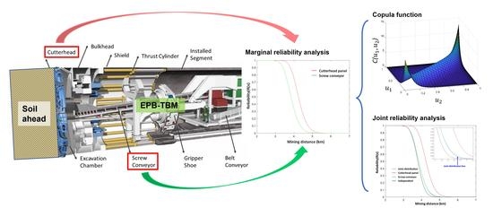
The data used in this research mainly include the remaining thickness for the wear-resistant material on the TBM’s key components, namely the cutter head panel and screw conveyor. In particular, the remaining thickness of the wear-resistance strip welded on the different sides of the cutter head panel was measured prior to and during tunnel excavation. The cutter head panel was evenly divided into several zones, with a few locations measured for each zone. To avoid data bias, the average value for each zone was calculated to represent the zone. Similarly, the screw conveyor was divided into several zones and the remaining thickness of the wear-resistance strips was measured at the same location as the cutter head panels. The collected data were used to analyze the service life of single components as well as the joint distribution of the overall service life prediction.
The marginal distribution functions describe the reliability of TBM components with respect to mining distance. To establish the copula model on the TBM lifetime prediction, it was critical to derive the marginal distribution function for all key components involved. However, the data obtained from the site were incomplete due to the limited site measurements available. To overcome this problem, a marginal distribution function with incomplete information was constructed by the following steps.
Figure 1. Flowchart of the developed approach for reliability assessment in complex systems.
Buildings 12 01959 g001
Step 1: We defined the remaining thickness of wear-resistance structures in the cutter head panel and screw conveyor over the mining distance x following a function y i ( x ) . In this function, i indicates the type of components (i = 1 for cutter head panel, i = 2 for screw conveyor). In this research, we assumed that the relationship between the mining distance and the remaining thickness for the cutter head panel or the screw conveyor was linear. This assumption was purely based on the observation of the data, and it might not be applicable to other cases. A different function can be proposed based on the nature of the collected data or estimated by means of the maximum likelihood methods [51]. In this study, the function was proposed as follows.
y i ( x ) = α i + β i x
where α indicates the initial thickness, β is the rate of wearing, and x is the mining distance. The normal distribution, Weibull distribution, Gumbel distribution, and logistics distribution were selected as candidate marginal distributions to describe the relationship between the remaining distance of the wear-resistance structure and the mining distance.
Step 2: For the normal distribution, i.e., α ~ N ( μ α i , σ α i 2 ) , β ~ N ( μ β i , σ β i 2 ) , y i ( x ) follows Equation (1). As α and β are independent, the mean and variance for function y i ( x ) can be expressed as follows:
μ ˜ i ( x ) = E { y i ( x ) } = μ α i + μ β i x
σ ˜ i ( x ) = V a r { y i ( x ) } = σ α i 2 + σ β i 2 x
where parameters from Equations (2) and (3) can be derived by finding out the best-fitting distribution based on TBM mining data.
Step 3: The function F i ( x ) was defined as the probability of the component malfunction, and the malfunction value for the cutter head panel and screw conveyor was set as H 1 and H 2 . If the thickness of the wear-resistance structure for these two components falls below the malfunction value, y 1 < H 1   o r   y 2 < H 2 , then the TBM is considered unreliable for work. Therefore, the function F i ( x ) is the cumulative density function (CDF) of y i < H i , and it is expressed as follows:
F i ( x ) = P ( y i ( x ) < H i ) = Φ ( H i μ ˜ i ( x ) σ ˜ i ( x ) ) = 1 2 π t ¯ e t 2 2 d t
where t ¯ = H i μ ˜ i ( x ) σ ˜ i ( x ) and Φ denote the expression in the bracket that follows the CDF of standard normal distribution.
Step 4: The function R i ( x ) was defined as the probability of component functions reliability. The probability for the component is 1 when the tunneling work just starts and gradually reduces with the increment of mining distance. That is, R i ( x ) reduces and F i ( x ) increases as the mining distance x increases. However, the total probability of component reliability and malfunction is always constant. Therefore, F i ( x ) + R i ( x ) = 1 , and R i ( x ) is expressed as
R i ( x ) = 1 F i ( x ) = P ( y i ( x ) H i ) = 1 Φ ( H i μ ˜ i ( x ) σ ˜ i ( x ) ) = 1 1 2 π t ¯ e t 2 2 d t
Step 5: The same procedure is repeated in steps 2–4 for the Weibull distribution and/or Gumbel distribution. However, the mean μ ˜ i ( x ) and variance σ ˜ i ( x ) for the normal distribution is replaced by the location parameter μ ˜ i ( x ) and scale parameter b ˜ i ( x ) for the Gumbel distribution, the shape parameter k i ˜ ( x ) and scale parameter λ ˜ i ( x ) for the Weibull distribution, and the location parameter μ ˜ i ( x ) and scale parameter s ˜ i ( x ) for logistic distribution. The reliability function for the Gumbel distribution, Weibull distribution, and logistic distribution can be expressed in Equations (6)–(8), respectively:
R i ( x ) = P ( y i ( x ) H i ) = e e ( x μ ˜ i ( x ) ) / b ˜ i ( x )
R i ( x ) = P ( y i ( x ) H i ) = e ( H i λ ˜ i ( x ) ) k ˜ i ( x )
R i ( x ) = P ( y i ( x ) H i ) = 1 1 + e ( H i μ ˜ i ( x ) ) / s ˜ i ( x )
where the location parameter μ ˜ i ( x ) = μ α i + μ β i x   and scale parameter b ˜ i ( x ) = b α i + b β i x   for the Gumbel distribution, shape factor k i ˜ ( x ) = k α i + k β i x , the scale parameter λ ˜ i ( x ) = λ α i exp ( λ β i ) + λ γ i for the Weibull distribution, and location parameter μ ˜ i ( x ) = μ α i + μ β i x   and scale parameter s ˜ i ( x ) = s α i + s β i x for the logistics distribution.
Step 6: The goodness of fit for candidate distributions should be estimated to determine the best fitting type of marginal distribution. Akaike Information Criteria (AIC) [52] and Bayesian Information Criteria (BIC) [53] are the two common measures for checking data fitness. AIC and BIC are estimators that can estimate the quality of each model, which is the best-fitting marginal distribution function. AIC and BIC values can be calculated based on the formulas below:
A I C = 2 i = 1 N l n f ( x ; μ , σ ) + 2 k
B I C = 2 i = 1 N l n f ( x ; μ , σ ) + k l n N
where k is the number of correlation parameters in the model, N is the number of data, and f ( x ; μ , σ ) is the maximum value of the likelihood function of the model. As Equations (9) and (10) suggest, the difference between AIC and BIC is that BIC gives more penalty when a greater number of correlation parameters are involved in the model under relatively big data size. However, as the parameters in candidate models are the same in this case, AIC and BIC values should be consistent. Therefore, the model should be selected when AIC and BIC values are the lowest among the candidate models.

3.2. Structural Learning for System Failure Models

The structure of the failure mode is critical for reliability analysis. The failure structure of the system is determined according to the mechanism and the relation between the components. Generally, serial, parallel, and mixed are the three essential relationships between the components in an engineering system [54]. If the components are in serial, the system will fail if any of its components fail. For a parallel system, the system will succeed if any of its components succeed. The mixed system is a more complicated system that contains both serial and parallel systems [55]. One of the useful tools to describe the relationship between the components and the overall system is the reliability block diagram (RBD) method. In this approach, the influential components are represented by blocks, and their relationships are denoted by the links in between. Given components 1, 2, …, i, and their marginal failure probability functions F 1 ( x ) , F 2 ( x ) , …, F i ( x ) , the joint failure probability is different if the components are constructed in different structures.
For a system that consists of two components, their relationship would be either serial or parallel. Figure 2 summarizes the RBD for a system with two components. The system follows failure mode (a) if the two components are in parallel and mode (b) if the two components are in serial. Apart from different failure modes, the dependency between each component affects the joint probability as well. For example, if the given system follows mode (a) and the two sub-systems are independent of each other, the reliability can be calculated as R ( x ) = ( 1 F 1 ( x ) ) ( 1 F 2 ( x ) ) = 1 F 1 ( x ) F 2 ( x ) + F 1 ( x ) F 2 ( x ) . However, if the two sub-systems are dependent, the reliability is calculated as R ( x ) = 1 C ( F 1 ( x ) , F 2 ( x ) ; θ 1 ) , where C denotes the copula function, and θ is the correlation parameter between the two marginal variables. Similarly, the general formula of the reliability function R i ( x ) under different failure mode structures and different dependency conditions (dependent or independent) can be calculated, respectively, and the results are shown in Table 2.
For the system that consists of three components, the relationship can be serial, parallel, or mixed. Figure 3 summarizes the RBD for a system with three components. Similar to the two component case, mode (a) and (b) describe the failure scenarios for the three component system, where mode (a) is for all components in parallel and mode (b) is for all in serial. However, there are three other possible failure modes described in (c), (d), and (e), where the components are in a mixed system. Different RBDs are formed based on the different critical paths of the components. Mode (c) is followed when two components ( F 1 ( x )   and   F 2 ( x ) ) are replaceable with each other while any of them can form a critical path with the other one ( F 3 ( x ) ). However, if there are two possible critical paths between the two components ( F 1 ( x )   and   F 2 ( x ) ) or F 3 ( x ) , mode (d) is followed. If the system can properly function when any two out of three components are working well, mode (e) describes such a situation. The reliability functions R i ( x ) for three components under different failure modes and dependencies are also summarized in Table 2. For instance, if a system has three components, then a failure of all causes the system to break down. In this case, these three components are in parallel and failure mode (a) in Table 2 is followed. As a result, the reliability function follows R ( x ) = 1 C ( F 1 ( x ) , F 2 ( x ) , F 1 ( x ) ; θ 1 θ 2 θ 3 ) .

3.3. Copula Enabled Data-Driven Prediction

Copulas are functions that describe the dependency between the n-dimensional multivariate joint distribution and 1-dimensional marginal functions, given that the probability distribution of these variables is uniform [56]. Derived by Sklar [57], given a d-dimensional CDF, F ( x 1 ,   x 2 ,   ,   x d   ) , with marginal functions F 1 ,   F 2 ,   ,   F d , a copula C exists, as shown below:
F ( x 1 ,   x 2 ,   ,   x d   ) = C ( F 1 ( x 1 ) ,   F 2 ( x 2 ) ,   ,   F d ( x d ) )
where all x i ϵ [ , ] and i = 1 ,   2 ,   ,   d . The copula function is unique if F i is continuous for all i = 1 ,   2 ,   ,   d . For the case of two variables, the formula can be rewritten as follows.
F ( x 1 , x 2 ) = C [ F 1 ( x 1 ) , F 2 ( x 2 ) ] = C ( u 1 , u 2 ; θ )
where C denotes the copula function, θ is the correlation parameter between the two marginal variables, and u 1 , u 2 refer to the marginal distribution functions for F 1 ,   F 2 , respectively. Therefore, the copula function is utilized to develop the reliability function model that includes dependent marginal variables.
There are three types of copula functions largely applied in engineering studies, namely Archimedean copulas, Elliptical copulas, and Vine copulas. Archimedean copulas are by far the most popular copulas due to their relatively simple structure, ease of calculation, and high adaptability and flexibility in engineering problems [58]. Therefore, Archimedean copulas were tested in this paper to find the most suitable copula type for the TBM service life prediction model. The selected candidate copulas are shown in Table 3 below.
Before the confirmation of the copula function, it is vital to analyze the dependence structure of copulas. There are three principles used to measure the dependence: Pearson correlation, rank correlation, and coefficient of tail dependence. Pearson correlation mainly measures the linear relationship between variables, while it is not suitable for non-linear conditions. Spearman’s rho and Kendall’s tau are the key values for rank correlation measures, and they are very useful in calibrating copula functions. Tail dependence was not necessary to be measured in this case. Therefore, Kendall’s tau was utilized to measure the dependence and correlation parameter θ. For two random variables X 1 and X 2 , Kendall’s tau ρ T is defined as
ρ T = ( N 2 ) 1 i < j s i g n [ ( x 1 i x 1 j ) ( x 2 i x 2 j ) ]
where s i g n ( · ) is defined as
s i g n = { 1   ( x 1 i x 1 j ) ( x 2 i x 2 j ) > 0 1   ( x 1 i x 1 j ) ( x 2 i x 2 j ) < 0   i , j = 1 ,   2 , ,   N
Based on the copula theory, the correlation parameter of copula θ can be calculated based on the following equation:
ρ T = 4 0 1 0 1 C ( μ 1 , μ 2 ; θ ) d C ( μ 1 , μ 2 ; θ ) 1
AIC and BIC are used to determine the best-fitting candidate copula models. AIC and BIC values for the copula model can be calculated based on the formula below.
A I C = 2 i = 1 N l n f ( μ 1 i , μ 2 i ; θ ) + 2 k
B I C = 2 i = 1 N l n f ( μ 1 i , μ 2 i ; θ ) + k l n N
where f ( u 1 i , u 2 i ; θ ) denotes the likelihood function and can be regarded as the density of the respective copula function, where f ( u 1 i , u 2 i ; θ ) = C ( u 1 , u 2 ; θ ) u 1 u 2 [59,60]. AIC and BIC values are calculated for each candidate copula function, and the one with the minimum AIC and BIC values is the best-fit model among the candidate copula models.
From Section 3.1, the remaining lifetime function for a single component is R i ( x ) = P ( y i ( x ) H i ) . Therefore, with the copula model developed in Section 3.2, the remaining lifetime function of the whole TBM can be expressed as below.
R ( x ) = P ( y 1 ( x ) H 1 ,   y 2 ( x ) H 2 ) = 1 P ( y 1 ( x ) < H 1 ) P (   y 2 ( x ) < H 2 ) + P ( y 1 ( x ) H 1 ,   y 2 ( x ) H 2 ) = 1 F 1 ( x ) F 2 ( x ) + C ( u 1 , u 2 ; θ )
where F 1 ( x ) , F 2 ( x ) are the marginal distribution function for the remaining lifetime of the wear-resistance structure in the cutter head panel and screw conveyor, respectively. C ( u 1 , u 2 ; θ ) is the copula function that indicates the probability of both components.

4. Case Study

In order to justify the applicability and effectiveness of the developed approach, real data from open literature were utilized for an example illustration. The data were collected in one of the EPB-TBM projects in the Chengdu metro system, China.

4.1. Case Background

There are various types of TBMs available on the market, including open mode TBM, slurry TBM, mix shield TBM, and EPB TBM. EPB TBM is widely used in tunnel construction under soft cohesive soil or mixed ground conditions [61,62]. The basic principle for EPB TBM is to use the excavated soil to counter-balance the earth’s pressure, which is achieved by filling the soil inside its working chamber [63]. During the mining process, the soil is crushed and excavated by the cutter head and is transported into the pressurized working chamber. The screw conveyor then transports the soil from the working chamber to the belt conveyor or muck buckets, and the ladder transports the excavated soil to the disposal point [64]. While excavating the soil, the jacking system supplies pressure and thrust force to push the whole TBM moving forward. A detailed illustration of EPB-TBM, including the key components and photos of the cutter head panel and the screw conveyor, is shown in Figure 4a–c, respectively. As both the cutter head and screw conveyor can be worn during the mining process, the probability of failure is increased when the excavation distance increases. Therefore, the reliability of TBM is the joint probability distribution developed based on the marginal distribution of the two components.
The data used in this study follow the literature [65], which was collected from the Chengdu metro system tunneling project. Two sets of data were collected regarding the remaining thickness of the wear resistance structure for the cutter head panel and screw conveyor. For the cutter head panel, the wear-resistance structure refers to the wear-resistance strip welded on the front, rear, and sides of the cutter head panel. These strips were under the same working environment and loading conditions. Moreover, strips at different locations had the same initial thickness and material properties. To avoid data insufficiency, cutter head panels were evenly divided into 12 zones, in which each zone had 30 degrees of area. For each zone, a few data points were captured, while the average value was taken with extreme data eliminated to represent the actual remaining thickness for this zone. For the screw conveyor, the wear-resistance strips were also welded on the screw conveyor as a wear-resistance structure to protect the conveyor. For this EPB-TBM, there were nine rounds of spiral in the screw conveyor, and each round of spiral was equally divided into 18 zones. Similar to the data collection process for the cutter head panel, the average value for each zone was calculated from the remaining thickness measured on each round of the spiral to represent the actual condition. The remaining thickness was measured at a mining distance of 0 km, 0.614 km, 1.546 km, and 2.762 km. Details of the collected data for both cutter head panel and screw conveyor are shown in Table 4 and Table 5 below.

4.2. Model Development

Based on the data shown in the table above, the respective parameters under different candidate marginal distributions discussed in Section 3 could be calculated by fitting the data into the respective distribution. With the derived parameters, the probability of failure at each mining distance can be calculated. The predicted mining distance can then be determined at the preferred reliability.
To further illustrate the procedure, the normal distribution was utilized as an example. From the original data from the cutter head panel and screw conveyor, the mean and variance at each mining distance were calculated as shown in Table 6. With the calculated mean and variance, the best-fitting regression line was derived and plotted in Figure 5a,b for the mean and variance, respectively. In particular, the dots in Figure 5a represent the original data collected for each zone of the cutter head panel and the screw conveyor, and the dots in Figure 5b are the variance of these data at different mining distances. Since the linear fitting line achieved a high coefficient of determination ( R 2 ) with the data (greater than 0.95 for both cutterhead and screw conveyor), it justifies that our assumption was reasonable based on the collected data. The respective parameters are shown in Table 7, where α and β denote the initial thickness and wearing rate for the wear-resistance strips.
Since the mean and variance at all mining distances are known, the cumulative probability of failure can be calculated based on Equations (4) and (5) are derived in Section 3.1. For example, at a mining distance of 4 km, the mean and variance for the cutter head were 1.37 mm and 0.54 mm, respectively. The reliability was calculated to be 0.75. Similarly, the reliability at all mining distances were calculated and plotted in Figure 6a. Similar to the normal distribution, data fit parameters for other candidate distributions are shown in Table 8, Table 9 and Table 10. Following Equations (6)~(8) derived in Section 3.1, the reliability curves for both the cutter head panel and screw conveyor under these distributions are plotted in Figure 6b–d, respectively.
Following the procedures mentioned in Section 3.1, AIC and BIC values were calculated to determine the best-fitting distribution for the data, and the results are shown in Table 11. In Table 11, the normal distribution has the smallest AIC and BIC values for both the cutter head panel and screw conveyor (bold font). Hence, the normal distribution was selected as the candidate marginal distribution for this case study. Considering a threshold value of H 1 = 1   mm , which is the minimum allowable thickness for the wear-resistance strips on both the cutter head panel and screw conveyor, the target reliability can be set at R ( x ) = 0.2 . That is to say, there is a high chance that the wear-resistance strips are less than 1 mm, which is unsafe if continues. However, the TBM itself is still safe at this point. From Figure 6, it is shown that the reliable mining distance for the cutter head and the screw conveyor under this setting is around 4.59 km and 4.18 km, respectively.
However, during the mining process, the soil is excavated by a cutter head and mixed with slurry. The slurry is then transported by a screw conveyor. The reliability and remaining thickness of the cutter head panel and screw conveyor are affected by some mutual parameters, such as the face pressure, thrust force, and soil excavation rate. Therefore, these two components are dependent, and the failure probability for TBM is the joint distribution depending on both marginal distributions of reliability. In this case, as two components are in serial, failure mode type (b), developed in Section 3.2, was followed. Moreover, the copula function was adopted to describe the dependency between the two marginal distributions. With the procedures described in Section 3.3, AIC and BIC values were calculated as shown in Table 12. With the AIC and BIC results, the Gumbel copula was considered the best-fitting candidate copula, as it possessed the smallest AIC and BIC values among these four candidate copula functions (bold font). Hence, the joint reliability function distribution was derived based on the Gumbel copula. The 3D plots of the probability density function (PDF) for different copulas are shown in Figure 7, where the surface of the figures indicates the probability of the copula function under the domain of [0,1].

4.3. Analysis of the Results

The joint distribution functions based on the Gumbel copula and other candidate copulas are plotted in Figure 8a–d, respectively. The line colored in blue is the joint distribution, and the lines colored in red and green are the marginal distributions for the cutter head panel and screw conveyors, respectively. However, the blue and red lines in Figure 8a,b are close to each other because the joint distribution and the screw conveyor’s marginal distribution are similar under the Gumbel and Gaussian copulas. The predicted mining distances at the reliability of 0.1, 0.2, and 0.3 for different copula models are shown in Table 13. The results indicate that the recommended reliable mining distance in this case study is 4.1652 km based on the reliability of 0.2. The predicted results are analyzed in detail below.
(1)
The results indicate that it is essential to consider the dependency between the wearing of the cutter head panel and the screw conveyor. It was shown that there is a strong positive correlation between the measured data of the two components. The predicted mining distance will not be accurate if the failure probability between the two components is assumed to be independent. From the results shown in this case study, the predicted mining distance would only be 3.9970 km if assuming independent. Compared with the result that incorporated the Gumbel copula function, the prediction is overly conservative and creates additional unnecessary costs due to CHI and cutting tool replacement. Therefore, the dependency between components was considered, and copula functions are the strong tool that could characterize the dependent structure. As shown in the case study, the predicted mining distance calculated based on candidate copula models vary from 4.0803 km to 4.0834 km, which is 2.08% and 2.16% higher than the independent assumption.
(2)
The developed reliability function curve is consistent with the data obtained from the site. From the data collected at a mining distance of 2.762 km, the remaining thickness of the wear resistance structure for both the cutter head panel and the screw conveyor were at an average of 3.15 mm and 2.36 mm, respectively. As all data collected at 2.762 km were much greater than 1 mm (mal-function value), these components were in good condition with 100% confidence. When reflecting on the reliability function curve, the reliability for both marginal distributions and joint distribution was 1. The remaining thickness kept dropping when the mining process persisted, the reliability curve started drop at 2.75 km and 3.25 km for screw conveyors and cutter head panels, and it reached 0 at a mining distance of 5 km and 5.5 km, respectively. This indicates that some wearing tools could have dropped to below 1 km between these mining distances and all would be below 1 mm at a distance of 5 km and 5.5 km. To keep a sufficient safety buffer, as well as to prevent being over-conservative, the reliability of 0.2 was selected for the mining distance prediction.
(3)
The screw conveyor is the key component that imposes a major contribution to the service life of TBM. This finding is based on the comparison between the two marginal distributions and the comparison with the joint distribution. Considering the two marginal distribution curves, it was shown that the cutter head panel was more reliable than the screw conveyor at the same mining distance. By comparing the marginal distribution curve and joint distribution curve, the joint distribution function line was the same as the reliability function of the screw conveyor when reliability was higher than 0.05. This shows that the screw conveyor could be the key component affecting the reliability of the whole TBM. However, when the mining distance was more than 4.5 km, the joint distribution curve moved away from the marginal distribution curve of the screw conveyor. This could be due to the dependency between the cutter head panel and the screw conveyor. In addition, although the joint reliability function was governed by the marginal reliability function of the screw conveyor, this does not mean that the screw conveyor is more important than the cutter head in terms of the tunnel excavation. Instead, the result generally indicates that the screw conveyor could be the bottleneck component in the system, and the overall performance of the TBM could be largely improved if a stronger screw conveyor is provided. A more detailed discussion on bottleneck detection is presented in Section 5.2.
(4)
Prediction results varied with different copulas selected. As shown in Figure 5, the types of copula functions affected the distribution of the joint PDF curve, which then resulted in different values at the same reliability. As reflected in Table 11, the values of the predicted mining distance varied from a minimum of 4.0803 km (Clayton copula) to a maximum value of 4.0834 km (Gumbel copula). As there is only a 0.76% difference between the maximum value to the minimum value, the selection of the copula function did affect the result significantly for this case study. The result could be because the joint reliability function of TBM is highly governed by the performance of the screw conveyor. Therefore, the observation from this case study may not be applicable to other cases. Hence, it is still recommended to select the most suitable copula function based on the AIC and BIC values calculated.

5. Discussions

Two significant factors affect the reliability of the predicted results, namely the structure of the failure mode and the marginal distribution of the components. For the failure mode structure, the prediction results vary largely if these components are in parallel instead of in serial. For marginal distribution, one component is the key influencing factor if the rate of wearing is huge. The system is optimized only if both components are equally reliable. Detailed discussions are presented below.

5.1. Influence of the System Structure

The failure mode structure can significantly affect the prediction result. As discussed in Section 3.2, a system with two components could be either in serial or parallel. The prediction result of 4.165 km was obtained based on the assumption that the components were in serial. However, the results were different if they were in parallel. The reliability R ( x ) was calculated as R ( x ) = 1 C ( F 1 ( x ) , F 2 ( x ) ; θ 1 ) in this case.
Figure 9 plots the reliability function with different failure mode structures (serial and parallel). Compared with serial failure mode, the prediction result for parallel was 4.576 km at the reliability level R ( x ) = 0.2 , with a 9.87% difference in prediction result. Therefore, it is critical to determine the failure mode before performing the calculation of the service life prediction or reliability. In this case study, the structure was clear and was easily determined, as only two components were involved in the study. However, for a complex system with a large number of components involved, the failure mode must be determined prior to the calculation. As discussed in Section 3.2, the user identifies the critical path for the components in the system and develops the RBD for the system. For example, for a system that consists of three components, the user needs to determine whether mode (e), (f), or (g) should be followed and decide which component is F 1 ( x ) , F 2 ( x ) , or F 3 ( x ) in the diagram. For a complex system, the user also determines the components that are dependent or independent of each other. A copula function should only be applied to those that are dependent on each other. The reliability function of the machinery could then be developed based on the RBD and dependency conditions between the components.

5.2. Influence of the Marginal Distribution

For the case study in Section 4, it can be seen that the joint distribution function was very close to the marginal distribution for the screw conveyor. The results indicate that the wear resistance structure in the screw conveyor could be the key factor that affects the service life of the entire TBM. Therefore, a further test is needed to justify the hypothesis of how the marginal distribution could affect the final prediction result. In this study, the initial thickness of the screw conveyor and cutter head panel increased by 0.5 mm, respectively, to test their contribution to the improvement of the overall reliability. Figure 10 shows the marginal distribution and joint distribution with the improved cutter head panel and screw conveyor.
In Figure 10, the plot reliability function curve indicates that the predicted mining distance increased significantly from 4.1652 km to 4.5075 km (8.22% increment) if the screw conveyor improved. However, there was no improvement in the TBM if the cutter head improved. Therefore, it can be concluded that the screw conveyor is the “bottleneck” of the system. Although an increment of 0.5 mm in thickness on the wear-resistance strips seems very negligible, the result was reasonable considering the scale of the original data. In specific, the wear-resistance strips of the screw conveyor had an average mean thickness of 5.83 mm before excavation and reduced to around 2.36 mm after excavation for around 2.76 km. Refer to Figure 5 for the data fit line; the wearing of the screw conveyor was around 1.26 mm/km. Therefore, by increasing the initial thickness of 0.5 km, the increment of the reliable excavating distance of around 0.35 km (from 4.1652 km to 4.5075 km) was reasonable. Instead of increasing the initial thickness, the predicted mining distance also increased significantly to 4.4875 km (7.74% increment) if the wear resistance material in a screw conveyor was replaced with stronger material ( u β i reduced to 1.1638 instead of 1.2638). Therefore, it is recommended to improve the performance of the screw conveyor in this case study, which could be achieved by either increasing the initial thickness or using a better wear-resistance material. In general, this model can help the user to identify the weakness of the components in the TBM.

6. Conclusions and Future Works

This research provides a data analysis approach to predict the mining distance of a TBM by assessing the reliability of each component and deriving the joint distribution with a copula function. The developed approach provides a recommended mining distance for the user to conduct the inspection and replace the unreliable components. It could help to eliminate the risk of sudden breakdown and prevent redundant cutter head intervention, which could further help to reduce the operational cost and improve the efficiency of tunneling works. The developed approach consists of 3 main steps, including (1) marginal distribution determination, (2) structural learning, and (3) adaptive prediction based on data analysis.
Real data from Chengdu metro system tunneling project were utilized to examine the feasibility and effectiveness of the developed approach, where the wear resistance structure in the cutter head panel and screw conveyor were identified as the key components that may cause the malfunction of a TBM. The results from this case study indicate that: (1) With the developed approach, normal distribution and Gumbel copula function were selected as the best fitting marginal distribution and copula function. The predicted reliable mining distance was 4.1652 km at the reliability equals 0.2. (2) The copula function is critical to be considered, as the predicted result was only 4.0521 km if assumed independent, which is over-conservative. (3) The wear resistance structure in the screw conveyor is the key factor that influenced the mining distance of the TBM in this case study. With an improvement in either initial structure thickness or the capability of wearing resistance, the reliable mining distance can increase to 4.5075 km instead of 4.0834 km. Therefore, the developed method could help the user to identify the “bottleneck” in the system and to improve the overall performance by eliminating the bottleneck with the least resources required.
However, there are several limitations in this study for continuous research and improvement. For one thing, the soil condition in this study was assumed to be homogeneous, and the influence of TBM operational parameters was not considered. The estimation will be inaccurate if there is a large variation in the geological condition or the key TBM operating parameters (e.g., huge change in cutterhead torque or thrust force, etc.) during the tunnel excavation, as the rate of wearing on the structure varies in such conditions. Therefore, future study is recommended to consider these factors and quantify the contribution of different factors such that the model will be more robust under complex condition. For another, it is also very important to evaluate and mitigate the TBM damages during excavation, and our future study will focus on optimizing TBM operational parameters using advanced multi-objective optimization algorithms [66,67] for enhanced safety and efficiency of TBM operations, particularly in complex geological conditions.

Author Contributions

Conceptualization, X.F. and L.Z.; methodology, X.F. and L.Z.; validation, L.Z.; formal analysis, X.F. and L.Z.; data curation, X.F. and L.Z.; writing—original draft preparation, X.F.; writing—review and editing, X.F., L.Z. and M.W.; visualization, X.F., L.Z. and M.W.; supervision, L.Z.; project administration, L.Z.; funding acquisition, L.Z. All authors have read and agreed to the published version of the manuscript.

Funding

This work is supported in part by the National Natural Science Foundation of China (Grant No. 72271101) and the Start-Up Grant at Huazhong University of Science and Technology (Grant No. 3004242122).

Data Availability Statement

The data involved in this study are presented in Table 4 and Table 5 of this paper.

Conflicts of Interest

The authors declare no conflict of interest.

References

  1. Zhang, L.; Zhang, Y.; Li, H.X.; Lei, Z. Estimating long-term impacts of tunnel infrastructure development on urban sustainability using granular computing. Appl. Soft Comput. 2021, 113, 107932. [Google Scholar] [CrossRef]
  2. Deng, M. Challenges and Thoughts on Risk Management and Control for the Group Construction of a Super-Long Tunnel by TBM. Engineering 2018, 4, 112–122. [Google Scholar] [CrossRef]
  3. Li, J.; Zhang, Z.; Meng, Z.; Huo, J.; Xu, Z.; Chen, J. Tunnel boring machine cutterhead crack propagation life prediction with time integration method. Adv. Mech. Eng. 2019, 11. [Google Scholar] [CrossRef] [Green Version]
  4. Wang, J.; Mohammed, A.S.; Macioszek, E.; Ali, M.; Ulrikh, D.V.; Fang, Q. A Novel Combination of PCA and Machine Learning Techniques to Select the Most Important Factors for Predicting Tunnel Construction Performance. Buildings 2022, 12, 919. [Google Scholar] [CrossRef]
  5. Elbaz, K.; Shen, S.-L.; Zhou, A.; Yin, Z.-Y.; Lyu, H.-M. Prediction of Disc Cutter Life During Shield Tunneling with AI via the Incorporation of a Genetic Algorithm into a GMDH-Type Neural Network. Engineering 2021, 7, 238–251. [Google Scholar] [CrossRef]
  6. Zhang, L.; Chettupuzha, A.A.; Chen, H.; Wu, X.; AbouRizk, S.M. Fuzzy cognitive maps enabled root cause analysis in complex projects. Appl. Soft Comput. 2017, 57, 235–249. [Google Scholar] [CrossRef]
  7. Li, X.; Yuan, D. Creating a working space for modifying and maintaining the cutterhead of a large-diameter slurry shield: A case study of Beijing railway tunnel construction. Tunn. Undergr. Space Technol. 2018, 72, 73–83. [Google Scholar] [CrossRef]
  8. Alavi Gharahbagh, E.; Mooney, M.A.; Frank, G.; Walter, B.; DiPonio, M.A. Periodic inspection of gauge cutter wear on EPB TBMs using cone penetration testing. Tunn. Undergr. Space Technol. 2013, 38, 279–286. [Google Scholar] [CrossRef]
  9. Amoun, S.; Sharifzadeh, M.; Shahriar, K.; Rostami, J.; Tarigh Azali, S. Evaluation of tool wear in EPB tunneling of Tehran Metro, Line 7 Expansion. Tunn. Undergr. Space Technol. 2017, 61, 233–246. [Google Scholar] [CrossRef]
  10. Huo, J.; Zhu, D.; Hou, N.; Sun, W.; Dong, J. Application of a small-timescale fatigue, crack-growth model to the plane stress/strain transition in predicting the lifetime of a tunnel-boring-machine cutter head. Eng. Fail. Anal. 2017, 71, 11–30. [Google Scholar] [CrossRef]
  11. Barzegari, G.; Uromeihy, A.; Zhao, J. Parametric study of soil abrasivity for predicting wear issue in TBM tunneling projects. Tunn. Undergr. Space Technol. 2015, 48, 43–57. [Google Scholar] [CrossRef]
  12. Ling, J.; Sun, W.; Huo, J.; Guo, L. Study of TBM cutterhead fatigue crack propagation life based on multi-degree of freedom coupling system dynamics. Comput. Ind. Eng. 2015, 83, 1–14. [Google Scholar] [CrossRef]
  13. Talebi, K.; Memarian, H.; Rostami, J.; Alavi Gharahbagh, E. Modeling of soil movement in the screw conveyor of the earth pressure balance machines (EPBM) using computational fluid dynamics. Tunn. Undergr. Space Technol. 2015, 47, 136–142. [Google Scholar] [CrossRef]
  14. Wang, S.; Li, H.; Tian, R.; Wang, R.; Wang, X.; Sun, Q.; Fan, J. Numerical simulation of particle flow behavior in a screw conveyor using the discrete element method. Particuology 2019, 43, 137–148. [Google Scholar] [CrossRef]
  15. Nelsen, R.B. An Introduction to Copulas, 2nd ed.; Springer Science+Business Media, Inc.: New York, NY, USA, 2006. [Google Scholar]
  16. Liu, X.-d.; Pan, F.; Cai, W.-l.; Peng, R. Correlation and risk measurement modeling: A Markov-switching mixed Clayton copula approach. Reliab. Eng. Syst. Saf. 2020, 197, 106808. [Google Scholar] [CrossRef]
  17. Favre, A.C.; El Adlouni, S.; Perreault, L.; Thiémonge, N.; Bobée, B. Multivariate hydrological frequency analysis using copulas. Water Resour. Res. 2004, 40, W01101. [Google Scholar] [CrossRef] [Green Version]
  18. Kole, E.; Koedijk, K.; Verbeek, M. Selecting copulas for risk management. J. Bank. Financ. 2007, 31, 2405–2423. [Google Scholar] [CrossRef] [Green Version]
  19. Fang, G.; Pan, R.; Hong, Y. Copula-based reliability analysis of degrading systems with dependent failures. Reliab. Eng. Syst. Saf. 2020, 193, 106618. [Google Scholar] [CrossRef]
  20. Qian, B.; Li, Z.-c.; Hu, R. A copula-based hybrid estimation of distribution algorithm for m-machine reentrant permutation flow-shop scheduling problem. Appl. Soft Comput. 2017, 61, 921–934. [Google Scholar] [CrossRef]
  21. Jin, R.; Wang, F.; Liu, D. Dynamic probabilistic analysis of accidents in construction projects by combining precursor data and expert judgments. Adv. Eng. Inform. 2020, 44, 101062. [Google Scholar] [CrossRef]
  22. Pan, Y.; Zhang, L.; Wu, X.; Qin, W.; Skibniewski, M.J. Modeling face reliability in tunneling: A copula approach. Comput. Geotech. 2019, 109, 272–286. [Google Scholar] [CrossRef]
  23. Tang, X.-S.; Li, D.-Q.; Zhou, C.-B.; Phoon, K.-K. Copula-based approaches for evaluating slope reliability under incomplete probability information. Struct. Saf. 2015, 52, 90–99. [Google Scholar] [CrossRef]
  24. Pan, Y.; Ou, S.; Zhang, L.; Zhang, W.; Wu, X.; Li, H. Modeling risks in dependent systems: A Copula-Bayesian approach. Reliab. Eng. Syst. Saf. 2019, 188, 416–431. [Google Scholar] [CrossRef]
  25. Lv, J.; Lin, D.; Wu, W.; Huang, J.; Li, Z.; Fu, H.; Li, H. Mechanical Responses of Slurry Shield Underpassing Existing Bridge Piles in Upper-Soft and Lower-Hard Composite Strata. Buildings 2022, 12, 1000. [Google Scholar] [CrossRef]
  26. Wang, L.; Kang, Y.; Zhao, X.; Zhang, Q. Disc cutter wear prediction for a hard rock TBM cutterhead based on energy analysis. Tunn. Undergr. Space Technol. 2015, 50, 324–333. [Google Scholar] [CrossRef]
  27. Bruland, A. Hard Rock Tunnel Boring Advance Rate and Cutter Wear; Norwegian Institute of Technology (NTNU): Trondheim, Norway, 1999. [Google Scholar]
  28. Rostami, J. Development of a Force Estimation Model for Rock Fragmentation with Disc Cutters through Theoretical Modeling and Physical Measurement of Crushed Zone Pressure; Colorado School of Mines Golden: Golden, CO, USA, 1997. [Google Scholar]
  29. Gehring, K. Prognosis of advance rates and wear for underground mechanized excavations. Felsbau 1995, 13, 439–448. [Google Scholar]
  30. Nelson, P.; Al-Jalil, Y.A.; Laughton, C. Tunnel Boring Machine Project Data Bases and Construction Simulation; Geotechnical Engineering Report GR94-4; The University of Texas at Austin: Austin, TX, USA, 1994; Volume 78712. [Google Scholar]
  31. Bieniawski, Z.; Celada, B.; Galera, J.; Tardáguila, I. Prediction of cutter wear using RME. In Proceedings of the ITA-AITES World Tunnel Congress, Budapest, Hungary, 25–27 May 2009. [Google Scholar]
  32. Liu, Q.; Liu, J.; Pan, Y.; Zhang, X.; Peng, X.; Gong, Q.; Du, L. A Wear Rule and Cutter Life Prediction Model of a 20-in. TBM Cutter for Granite: A Case Study of a Water Conveyance Tunnel in China. Rock Mech. Rock Eng. 2017, 50, 1303–1320. [Google Scholar] [CrossRef]
  33. Hassanpour, J.; Rostami, J.; Tarigh Azali, S.; Zhao, J. Introduction of an empirical TBM cutter wear prediction model for pyroclastic and mafic igneous rocks; a case history of Karaj water conveyance tunnel, Iran. Tunn. Undergr. Space Technol. 2014, 43, 222–231. [Google Scholar] [CrossRef]
  34. Oñate Salazar, C.G.; Todaro, C.; Bosio, F.; Bassini, E.; Ugues, D.; Peila, D. A new test device for the study of metal wear in conditioned granular soil used in EPB shield tunneling. Tunn. Undergr. Space Technol. 2018, 73, 212–221. [Google Scholar] [CrossRef] [Green Version]
  35. Alber, M.; Yaralı, O.; Dahl, F.; Bruland, A.; Käsling, H.; Michalakopoulos, T.N.; Cardu, M.; Hagan, P.; Aydın, H.; Özarslan, A. ISRM Suggested Method for Determining the Abrasivity of Rock by the CERCHAR Abrasivity Test. Rock Mech. Rock Eng. 2014, 47, 261–266. [Google Scholar] [CrossRef]
  36. Thuro, K.; Singer, J.; Käsling, H.; Bauer, M. Soil abrasivity assessment using the LCPC testing device. Felsbau 2006, 24, 37–45. [Google Scholar]
  37. Blindheim, O.; Bruland, A. Boreability testing. Nor. TBM Tunn. 1998, 30, 29–34. [Google Scholar]
  38. Cardu, M.; Iabichino, G.; Oreste, P.; Rispoli, A. Experimental and analytical studies of the parameters influencing the action of TBM disc tools in tunnelling. Acta Geotech. 2016, 12, 293–304. [Google Scholar] [CrossRef]
  39. Jakobsen, P.D.; Langmaack, L.; Dahl, F.; Breivik, T. Development of the Soft Ground Abrasion Tester (SGAT) to predict TBM tool wear, torque and thrust. Tunn. Undergr. Space Technol. 2013, 38, 398–408. [Google Scholar] [CrossRef]
  40. Ren, D.-J.; Shen, J.S.; Chai, J.-C.; Zhou, A. Analysis of disc cutter failure in shield tunnelling using 3D circular cutting theory. Eng. Fail. Anal. 2018, 90, 23–35. [Google Scholar] [CrossRef]
  41. Li, G.; Wang, W.; Jing, Z.; Zuo, L.; Wang, F.; Wei, Z. Mechanism and numerical analysis of cutting rock and soil by TBM cutting tools. Tunn. Undergr. Space Technol. 2018, 81, 428–437. [Google Scholar] [CrossRef]
  42. Owen, P.J.; Cleary, P.W. Prediction of screw conveyor performance using the Discrete Element Method (DEM). Powder Technol. 2009, 193, 274–288. [Google Scholar] [CrossRef]
  43. Geng, Q.; Wei, Z.; Ren, J. New rock material definition strategy for FEM simulation of the rock cutting process by TBM disc cutters. Tunn. Undergr. Space Technol. 2017, 65, 179–186. [Google Scholar] [CrossRef]
  44. Pan, Y.; Zhang, L. Roles of artificial intelligence in construction engineering and management: A critical review and future trends. Autom. Constr. 2021, 122, 103517. [Google Scholar] [CrossRef]
  45. Zhang, L.; Wu, X.; Ji, W.; AbouRizk, S.M. Intelligent Approach to Estimation of Tunnel-Induced Ground Settlement Using Wavelet Packet and Support Vector Machines. J. Comput. Civ. Eng. 2017, 31, 04016053. [Google Scholar] [CrossRef]
  46. Crk, V. Reliability assessment from degradation data. In Proceedings of the Annual Reliability and Maintainability Symposium. 2000 Proceedings. International Symposium on Product Quality and Integrity, Los Angeles, CA, USA, 24–27 January 2000; pp. 155–161. [Google Scholar]
  47. Zhao, C.; Zhuang, G.; Du, Z.; Sui, S. The data mining method based on support vector machine applied to predict tool life of TBM. In Proceedings of the 2017 29th Chinese Control and Decision Conference (CCDC), Chongqing, China, 28–30 May 2017; pp. 3439–3444. [Google Scholar] [CrossRef]
  48. Zhang, L.; Wu, X.; Skibniewski, M.J. Simulation-Based Analysis of Tunnel Boring Machine Performance in Tunneling Excavation. J. Comput. Civ. Eng. 2016, 30, 04015073. [Google Scholar] [CrossRef]
  49. Gouarir, A.; Martínez-Arellano, G.; Terrazas, G.; Benardos, P.; Ratchev, S. In-process Tool Wear Prediction System Based on Machine Learning Techniques and Force Analysis. Procedia CIRP 2018, 77, 501–504. [Google Scholar] [CrossRef]
  50. Zhang, X.; Lin, L.; Xia, Y.; Tan, Q.; Zhu, Z.; Mao, Q.; Zhou, M. Experimental study on wear of TBM disc cutter rings with different kinds of hardness. Tunn. Undergr. Space Technol. 2018, 82, 346–357. [Google Scholar] [CrossRef]
  51. Shinozuka, M.; Feng, M.Q.; Lee, J.; Naganuma, T. Statistical Analysis of Fragility Curves. J. Eng. Mech. 2000, 126, 1224–1231. [Google Scholar] [CrossRef] [Green Version]
  52. Akaike, H. A new look at the statistical model identification. IEEE Trans. Autom. Control 1974, 19, 716–723. [Google Scholar] [CrossRef]
  53. Schwarz, G. Estimating the Dimension of a Model. Ann. Stat. 1978, 6, 461–464. [Google Scholar] [CrossRef]
  54. Bourouni, K. Availability assessment of a reverse osmosis plant: Comparison between Reliability Block Diagram and Fault Tree Analysis Methods. Desalination 2013, 313, 66–76. [Google Scholar] [CrossRef]
  55. Hu, C.; Wang, P.; Youn, B.D. Advances in System Reliability Analysis Under Uncertainty. In Numerical Methods for Reliability and Safety Assessment: Multiscale and Multiphysics Systems; Kadry, S., El Hami, A., Eds.; Springer International Publishing: Cham, Switzerland, 2015; pp. 271–303. [Google Scholar] [CrossRef]
  56. Trivedi, P.K. Copula Modeling: An Introduction for Practitioners; Now: Boston, MA, USA, 2007. [Google Scholar]
  57. Sklar, A. Random variables, joint distribution functions, and copulas. Kybernetika 1973, 9, 449–460. [Google Scholar]
  58. Savu, C.; Trede, M. Goodness-of-fit tests for parametric families of Archimedean copulas. Quant. Financ. 2008, 8, 109–116. [Google Scholar] [CrossRef]
  59. Durrleman, V.; Nikeghbali, A.; Roncalli, T. Which copula is the right one? SSRN 2000, 17, 1032545. [Google Scholar] [CrossRef] [Green Version]
  60. Gülöksüz, Ç.T. Comparison of some selection criteria for selecting bivariate archimedean copulas. Afyon Kocatepe Üniversitesi Fen Ve Mühendislik Bilim. Derg. 2016, 16, 250–255. [Google Scholar] [CrossRef]
  61. Wang, L.; Sun, W.; Long, Y.; Yang, X. Reliability-Based Performance Optimization of Tunnel Boring Machine Considering Geological Uncertainties. IEEE Access 2018, 6, 19086–19098. [Google Scholar] [CrossRef]
  62. Ergun, O.A.; Erdoğan, C.; Ekinci, E. Analysis of the EPB-TBM Excavation Parameters Used in a Tunnel Construction in Istanbul. In Proceedings of the 2nd World Congress on Mechanical, Chemical, and Material Engineering, Budapest, Hungary, 22–23 August 2016. [Google Scholar]
  63. Tatiya, R. Surface and Underground Excavations Methods, Techniques and Equipment, 2nd ed.; CRC Press/Balkema: Boca Raton, FL, USA, 2013. [Google Scholar]
  64. Hemphill, G.B. Tunnel-Boring Machines. In Practical Tunnel Construction; John Wiley & Sons: Hoboken, NJ, USA, 2012; pp. 171–185. [Google Scholar] [CrossRef]
  65. Dai, W. Research on Reliability Accessment and Residual Service Life Prediction of Key Components of Shield Machine Applied in Sandy Cobble Stratum. Master’s Thesis, Southwest Jiaotong University, Chengdu, China, 2014. [Google Scholar]
  66. Guo, K.; Zhang, L. Multi-objective optimization for improved project management: Current status and future directions. Autom. Constr. 2022, 139, 104256. [Google Scholar] [CrossRef]
  67. Zhang, L.; Lin, P. Multi-objective optimization for limiting tunnel-induced damages considering uncertainties. Reliab. Eng. Syst. Saf. 2021, 216, 107945. [Google Scholar] [CrossRef]
Figure 2. Structure of different failure models for two components: (a) in the parallel mode and (b) in the serial mode.
Buildings 12 01959 g002
Figure 3. Structure of different failure modes for three components: (a) in parallel; (b) in serial; and (ce) in a mixed system.
Buildings 12 01959 g003
Figure 4. Illustration of EPB-TBM for (a) key components in the TBM, (b) photo of the cutter head panel, and (c) photo of the screw conveyor.
Buildings 12 01959 g004
Figure 5. Fitted regression lines of the cutter head and screw conveyor at different mining distances: (a) mean values; (b) variance values.
Buildings 12 01959 g005
Figure 6. Marginal reliability function for the cutter head and screw conveyor under (a) normal distribution; (b) Weibull distribution; (c) Gumbel distribution; and (d) logistics distribution.
Buildings 12 01959 g006
Figure 7. The 3D plot of PDF for the joint distribution by (a) Gumbel copula; (b) Gaussian copula; (c) Clayton copula; and (d) Frank copula.
Buildings 12 01959 g007
Figure 8. Joint distribution of reliability function by (a) Gumbel copula; (b) Gaussian copula; (c) Clayton copula; and (d) Frank copula.
Buildings 12 01959 g008
Figure 9. Joint distribution of the reliability function with serial or parallel failure modes.
Buildings 12 01959 g009
Figure 10. Joint distribution of the reliability function with (a) the modified cutter head and (b) the modified screw conveyor.
Buildings 12 01959 g010
Table 1. Summary of major abrasivity test methods.
TestDescriptionReference
NTNU soil abrasion testSoil abrasivity is estimated based on the loss of steel pieces in the test device after a designed amount of oven-dried soil power sample flows through this test device. [37]
LPCP abrasimeter testThe test uses a metal impeller to crush the soil sample and sample abrasivity is measured based on the wearing of the metal impeller. [36]
Cerchar testThe test can obtain the Cerchar abrasivity index (CAI) by measuring the wearing of a steel stylus that moves into the rock sample at a certain force. [35]
Table 2. Joint distribution functions for a system consisting of two and three components under different failure modes and dependency conditions.
No of Components Mode Reliability   Function   R i ( x )   ( Independent ) Reliability   Function   R i ( x )   ( Dependent )
Two(a) 1 F 1 ( x ) F 2 ( x ) 1 C ( F 1 ( x ) , F 2 ( x ) ; θ 1 )
(b) 1 F 1 ( x ) F 2 ( x ) + F 1 ( x ) F 2 ( x ) 1 F 1 ( x ) F 2 ( x ) + C ( F 1 ( x ) , F 2 ( x ) ; θ 1 )
Three(a) 1 F 1 ( x ) F 2 ( x ) F 1 ( x ) 1 C ( F 1 ( x ) , F 2 ( x ) , F 1 ( x ) ; θ 1 θ 2 θ 3 )
(b) 1 F 1 ( x ) F 2 ( x ) F 3 ( x ) + F 1 ( x ) F 2 ( x ) + F 1 ( x ) F 2 ( x ) + F 1 ( x ) F 2 ( x ) F 1 ( x ) F 2 ( x ) F 1 ( x ) 1 F 1 ( x ) F 2 ( x ) F 3 ( x ) + C ( F 1 ( x ) , F 2 ( x ) ; θ 1 ) + C ( F 1 ( x ) , F 3 ( x ) ; θ 2 ) + C ( F 2 ( x ) , F 3 ( x ) ; θ 3 ) C ( F 1 ( x ) , F 2 ( x ) , F 1 ( x ) ; θ 1 θ 2 θ 3 )
(c) F 1 ( x ) F 2 ( x ) F 1 ( x ) F 2 ( x ) F 3 ( x ) C ( F 1 ( x ) , F 2 ( x ) ; θ 1 ) C ( F 1 ( x ) , F 2 ( x ) , F 1 ( x ) ; θ 1 θ 2 θ 3 )
(d) 1 F 3 ( x ) + F 1 ( x ) F 3 ( x ) + F 2 ( x ) F 3 ( x ) F 1 ( x ) F 2 ( x ) F 3 ( x ) 1 F 3 ( x ) + C ( F 1 ( x ) F 3 ( x ) ; θ 2 ) + C ( F 2 ( x ) F 3 ( x ) ; θ 3 ) C ( F 1 ( x ) F 2 ( x ) F 3 ( x ) ; θ 1 θ 3 )
(e) 1 F 1 ( x ) F 2 ( x ) F 1 ( x ) F 3 ( x ) F 2 ( x ) F 3 ( x ) + 2 F 1 ( x ) F 2 ( x ) F 3 ( x ) 1 C ( F 1 ( x ) F 2 ( x ) ; θ 1 ) C ( F 1 ( x ) F 3 ( x ) ; θ 2 ) C ( F 2 ( x ) F 3 ( x ) ; θ 3 ) + 2 C ( F 1 ( x ) F 2 ( x ) F 3 ( x ) ; θ 1 θ 2 θ 3 )
Table 3. Selected Archimedean copulas for testing.
Copula Type Copula   Function   C ( u 1 , u 2 ; θ ) Generator   φ ( t , θ ) θ
Gaussian Φ 1 ( u 1 ) Φ 2 ( u 2 ) 1 2 π 1 θ 2 e x p [ x 1 2 2 θ x 1 x 2 + x 2 2 2 ( 1 θ 2 ) ] d x 1 d x 2 [ 1 , 1 ]
Clayton ( u 1 θ + u 2 θ 1 ) 1 / θ φ θ ( t ) = 1 θ ( t θ 1 ) [ 0 , ]
Frank 1 θ l n ( 1 + ( e θ u 1 1 ) ( e θ u 2 1 ) e θ 1 ) l n e θ t 1 e θ 1 ( , ) \ { 0 }
Gumbel e x p { [ ( l n u 1 ) θ + ( l n u 2 ) θ ] 1 / θ }   φ θ ( t ) = ( l n t ) θ [ 1 , ]
Table 4. The remaining thickness for the wear-resistance structure on the cutter head panel.
ZoneRemaining Thickness (mm) at Different Mining Distances
0 km0.614 km1.546 km2.762 km
17.626.245.122.72
27.526.565.363.08
37.686.085.383.08
47.566.445.783.24
57.486.325.742.7
67.66.565.683.2
77.766.065.163.7
87.686.265.53.4
97.546.065.322.5
107.566.425.483.92
117.546.345.282.98
127.646.245.783.36
Table 5. The remaining thickness for the wear-resistance structure on the screw conveyor.
ZoneRemaining Thickness (mm) at Different Mining Distances
0 km0.614 km1.546 km2.762 km
15.925.33.822.24
26.004.743.622.76
35.845.263.561.94
45.745.043.362.9
55.5853.32.14
65.805.223.442.28
75.664.863.422.48
85.884.83.282.56
95.944.944.032.06
105.865.203.702.6
115.724.73.462.86
125.765.063.31.8
135.824.723.362.33
145.945.073.562.56
156.005.033.82.82
165.845.143.42.62
175.665.244.071.60
185.845.083.362.44
Table 6. Data fit mean and variance for the cutter head panel and screw conveyor under the normal distribution.
ComponentParametersMining Distances
0 km0.614 km1.546 km2.762 km
Cutter head panelMean7.59836.29835.46503.1567
Variance0.08070.17670.23500.4113
Screw conveyorMean5.83835.05003.52582.3600
Variance0.11420.17710.24040.3391
Table 7. Mean and variance for the cutter head panel and screw conveyor under the normal distribution.
Parameter Componentμaiσaiμβiσβi
Cutter head panel7.5420.11431.53800.0853
Screw conveyor5.74990.11971.26380.0796
Table 8. Shape and scale parameters for the cutter head panel and screw conveyor under the Weibull distribution.
Parameter Componentkaikβiλaiλβiλγi
Cutter head panel7.56611.490982.541.50211.6
Screw conveyor5.8111.229855.471.0092.852
Table 9. Location and scale parameters for the cutter head panel and screw conveyor under the Gumbel distribution.
Parameter Componentμaibaiμβibβi
Cutter head panel7.63860.08051.53540.1660
Screw conveyor5.88870.08721.59670.2153
Table 10. Mean and variance for the cutter head panel and screw conveyor under the logistics distribution.
Parameter Componentμaisaiμβisβi
Cutter head panel7.59320.04521.54190.1023
Screw conveyor5.84740.06071.46980.1324
Table 11. AIC and BIC values for the cutter head panel and screw conveyor under different distributions. The bold fonts generally indicate the lowest values in the table.
DistributionMeasuresCutter Head PanelScrew Conveyor
NormalAIC 2.009 × 10 4 1.529 × 10 4
BIC 2.010 × 10 4 1.530 × 10 4
WeibullAIC 2.418 × 10 4 1.644 × 10 4
BIC 2.418 × 10 4 1.644 × 10 4
GumbelAIC 2.813 × 10 4 7.101 × 10 4
BIC 2.814 × 10 4 7.101 × 10 4
LogisticsAIC 3.445 × 10 4 2.121 × 10 4
BIC 3.445 × 10 4 2.122 × 10 4
Table 12. AIC and BIC values for different copula types. The bold fonts generally indicate the lowest values in the table.
ItemGaussianFrankClaytonGumbel
AIC Value 1.515 × 10 3 2.547 × 10 3 3.959 × 10 3 2.605 × 10 3
BIC Value 1.510 × 10 3 2.542 × 10 3 3.960 × 10 3 2.600 × 10 3
Table 13. Predicted mining distances (unit: km) under different copulas, independent conditions, and marginal distributions.
Dependency StructurePredicted Mining Distance at Different Reliability Levels (km)
Reliability = 0.1Reliability = 0.2Reliability = 0.3
DependentGumbel copula4.26534.08343.9543
Gaussian copula4.26534.08073.9543
Clayton copula4.26144.08033.9545
Frank copula4.26494.08043.9546
Independent Joint4.13713.99703.8919
Screw conveyor 4.26554.08363.9546
Cutter head panel 4.76284.56764.4424
Publisher’s Note: MDPI stays neutral with regard to jurisdictional claims in published maps and institutional affiliations.

