Uncertainty Analysis of Inverse Problem of Resistivity Model in Internal Defects Detection of Buildings

Abstract

Fissure detection in ancient buildings is of vital importance in the evaluation of resistance or remediation in urban areas. Electrical resistivity imaging is an efficient tool to detect fissures or moisture erosion in buildings by highlighting the resistivity contrasts in the inversion models. The traditional results of ERT images give deterministic interpretations of the internal artifact. However, the existence of equivalent models may correspond to different physical realities in engineering cases, to which the traditional ERT model cannot respond. In this paper, through the application of a field test on an ancient wall, it is shown that the segmentation of the equivalent model family is applicable to solve the internal defects detection problem in a probabilistic approach. It is achieved by performing a probabilistic approach to apply the uncertainty analysis. The procedure begins with the reduction in dimensions of the model by spectral decomposition, and the uncertainty space is rebuilt via Particle Swarm Optimization (PSO). By computing the uncertainty space, probabilistic maps are created to demonstrate the electrical anomaly in a simpler structure. The proposed method provides a more accurate approach for the internal defects detection of buildings by considering the possibilities hidden in the equivalent model family of ERT results.

1. Introduction

Buildings deteriorate over the course of their service life. The enclosure, especially the walls, becomes significantly vulnerable due to defending against natural erosion. Before severe damage occurs, early-stage defects appear on the façade of the walls, such as fissures, cracks, or moisture erosion, easily observed on the walls of ancient buildings or even urban heritage sites [1,2]. However, some defects occur inside the wall, under the sub-surface of the building facade. The detection of hidden defects is necessary to prevent the total crack of the walls or even the structure.

Several methods are available for defect detection. Invasive methods, such as the carbide, Karl Fisher chemical method, and geotechnical method [3], may cause additional damage to the walls. In this case, non-invasive methods, including ground-penetrating radar [4], neutrons, nuclear magnetic resonance [5], spectral method [6], infrared thermography [7], optical method [8,9,10], microwaves [11], and electrical resistivity tomography [12,13], are adapted for defect detection in walls. Direct methods (borehole logging, geological mapping, GPS monitoring) or indirect methods (seismic refraction and reflection and electrical resistivity tomography) have their advantages and limitations [14,15,16]. In 1990, micro-seismic surveys had already been used to perform the detection of internal fissures on rock structures in Italy [17]. This study proves that the seismic survey is capable of locating the internal fissure in stone structures. Another project used the seismic method and numerical simulation to study the physical behavior of underground stations and also the interaction between the surface and buildings [18]. Crack detection can also be affected by the multi-component GPR method. The results show good coincidence with a priori information about the structure. Shadowed anomalies agree with the visualization on the tilling. However, the results are influenced by the presence of metallic mesh and the changes in coupling of antennas, which show the failure of the monitoring aspect [4]. Thermography is also an efficient tool to detect building defects. Compared with traditional walk-through technology, it is much quicker and cheaper, but it may miss some defect types [7].

The studies mentioned in the above paragraph showed that the detection of internal defects in walls can be affected by different kinds of noninvasive methods. Among the geophysical prospecting method, Electrical Resistivity Tomography (ERT) enables the efficient identification of defects in structures or geological domains without disturbing the original structure. As an area method, it can give spatial tomography images of the survey area and has been widely applied in geosciences [19,20,21], geotechnical studies [22], cavity detection, and hydrogeological studies. The method consists of performing a given set of injections of electrical current into the survey field (walls in the present study) and measuring the potential difference of each injection in a pre-defined acquisition set-up. From the mathematical point of view, the algorithm’s task is to solve the inverse problem, in which the resistivity or conductivity field is unknown. For this inverse problem, the number of equations equals the product of injections and the number of measurements taken during the data acquisition. Mathematical equations cope poorly with functions in which the number of arguments is less than dependent variables. Therefore, to solve the inverse problem, the solution of forward problems, whose number equals the injections performed during the survey, is required. Uncertainty analysis is then used to analyze the efficiency and accuracy of the solution to ill-posed questions. In addition, the noise of the data has its own impact on the uncertainty analysis. The effect of the noise and Tikhonov’s regularization have been studied by several scholars. It may enter the cost function of the inverse problem and perturb the finding of the true location of the inverse models [23,24]. The traditional ERT model is a deterministic interpretation of the inversion model. Due to the existence of multi-solutions (ill-posed problems) in the inversion problem, the equivalent models may exist. Therefore, an uncertainty analysis is required to determine whether the equivalent models will affect the interpretation of the engineering context.

The uncertainty analysis has been performed on different kinds of inverse problems. In the 1-D inverse problem, Carter et al. used the Hybrid Monte Carlo method to perform a joint inversion of electromagnetic survey data. It can avoid the random pitfalls during the inversion [25]. The geostatistical method for the uncertainty quantification of geothermal exploitation demonstrates that the uncertainty is highly related to the data density [26]. However, the analysis may expend several days for a global search. Karolczuk and Kurek proposed a life-time prediction of steel based on the Markov chain Monte Carlo method [27]. Furthermore, in electromagnetic inversion problems, the geometric sampling approach can be used to perform dimension reduction. In addition, Smolyak grids, a deterministic approach, could provide similar sampling results as Monte Carlo methods [28,29]. In most of the above studies, Monte Carlo methods are used for model space sampling and their time complexity is high. However, machine learning algorithms can accelerate the sampling or optimization progress by performing parallel computations using multiple CPUs and GPUs. The popular machine learning algorithm that can be used in the model sampling include sparse Bayesian learning [30], Linear Regression and Least-Angle Regression [31], Artificial Neural Networks (ANN) [32], Logistic Regression, Support Vector Machines (SVM), etc.

In this paper, we firstly review the inverse problems (ill-posed problems) in the resistivity electrical tomography. Then, we explain the approaches used in the uncertainty analysis. It is noted that a total Bayesian analysis requires a truly random sampling of the research space. If the dimension of the parameter spaces is high, the proposed approaches are unfeasible because of the costly forward problems. We apply the present method to a dataset, re-built from field data on a detection of wall defects, by adding a random level of noise. The analysis procedure consists of both the reduction in dimension by SVD and the model sampling. The equivalent resistivity model, in a probabilistic way, shows its potential to improve the quality of the geotechnical and geophysical interpretation. Compared with the existing state-of-the-art algorithm, the proposed method achieves a better understanding of the ERT model. An enhanced interpretation can be obtained by exploiting the probabilistic equivalent model family.

2. Inverse Problem and Uncertainty Analysis on Reduced Basis

2.1. Inverse Problem

Given a building or geological domain Ω ⸦ R² in its conductivity field σ, the forward problem of an electrical survey can be written as [33]:

$$F(\mathsf{\sigma })\cdot \mathbf{u}=\mathbf{q}$$

(1)

in which F denotes the forward operator, σ describes the conductivity vector in Ω, u denotes the potential vector in the field, and the vector q records the coordinates of both current injections. It should be noted that the conductivities in the forward problem are known, and the solution targets are the potentials.

However, the problem changes in real cases. The potentials are known, and the problem consists of finding the conductivity model σ of the field, which helps to interpret the geological setting of building environment of the survey field. To solve the inverse problem, a cost function C(σ) is defined:

$$C(\mathsf{\sigma })={\Vert \mathit{Q}{(F(\mathsf{\sigma }))}^{-1}\cdot \mathbf{q}-{\mathbf{d}}_{\mathrm{obs}}\Vert }_p+\epsilon \cdot {\Vert \mathsf{\sigma }-{\mathsf{\sigma }}_{\mathrm{ref}}\Vert }_q$$

(2)

To achieve the final model, the inverse problem consists of finding a minimum value of C(σ). In this function, $\epsilon \cdot {\Vert \mathsf{\sigma }-{\mathsf{\sigma }}_{\mathrm{ref}}\Vert }_q$ is the 0-order Tikhonov regularization term. This term imposes a compromise between the error ${\Vert \mathit{Q}{(F(\mathsf{\sigma }))}^{-1}\cdot \mathbf{q}-{\mathbf{d}}_{\mathrm{obs}}\Vert }_p$ and the reference model σ_ref. Moreover, 1- and 2-order Tikhonov regularizations can both be used; however, by giving different transition modes between conductivities in the model σ, it was proved the L1 norm can promote solutions in inverse problems whose boundary is abrupt and sparse [34]. The damping factor is mostly used to look for the minimum value of the data error to the reference model. The value of factor ε depends on the quality of the dataset and the noise level in the survey data. An empirical range for the value of ε is from 10⁻³ to 10⁻⁸. The increase in ε results in finding a simpler and smoother solution but with the augmentation of model misfits’ levels. Besides, an excessive increase in the grid number and an inappropriate choice for the size of the grid could both add uncertainty to the final model [35].

2.2. Uncertainty Analysis in Reduced Specter Basis

Finer discretization of the model grid is often used to increase the accuracy of the obtention in the final model. However, this could lead to a quick augmentation in the dimensionality of the inverse problem. In a 2D case, the parameters of inversion can easily reach up to 1000. Therefore, the regularization term mentioned in the upper part aims at stabilizing the inversion by avoiding the appearance of under-determined parameters. Nevertheless, the regularization itself cannot prevent the extension of the equivalent model space. The noise level could also perturb the inverse procedure. Therefore, an uncertainty analysis for the optimal model is needed for evaluation. In this paper, a Bayesian uncertainty analysis of the ERT inverse problem is presented. Assuming that the optimal solution for the tomographic inverse problem is obtained by local optimization methods, the methodology consists of three steps, as shown below.

2.2.1. Spectral Decomposition of the Inverse Model

Given a model σ ∈ R^m,n, m and n are the number of rows and columns in the data matrix of σ, corresponding, respectively, to the number of cells in the discretization model. By applying the Singular Value Decomposition (SVD) [36], the matrix σ can be transformed into the following form:

$$\mathsf{\sigma }=\mathbf{U}\mathsf{\Sigma }{\mathbf{V}}^T={\displaystyle \sum _{i=1}^r{\mathsf{\alpha }}_i{\mathbf{u}}_i{\mathbf{v}}_i{}^T}$$

(3)

where ${\mathsf{\alpha }}_i$ is the vector of singular values of σ. Equation (3) gives the spectral decomposition of σ, which demonstrates that the conductivity (or resistivity) model σ can be expanded on an r spectral basis with the term ${\mathbf{u}}_i{\mathbf{v}}_i{}^T$. In this case, the total information contained in the model σ is explained by:

$${\Vert \mathsf{\sigma }\Vert }_F=\sqrt{{\displaystyle \sum _{i=1}^r{\mathsf{\alpha }}_i{}^2}}$$

(4)

where ${\Vert \mathsf{\sigma }\Vert }_F$ is the Frobenius norm of σ. In Equation (4), the number of basis terms k (≤ r) can be chosen by calculating the loss tolerance L of information after the expansion of σ, as follows:

$$L\ge \frac{{\Vert \mathsf{\sigma }\Vert }_F-\sqrt{{\displaystyle \sum _{i=1}^k{\mathsf{\alpha }}_i{}^2}}}{{\Vert \mathsf{\sigma }\Vert }_F}$$

(5)

To choose the number of basic terms k, we define a tolerance level L, as in Equation (5). Mathematically, it is recommended to define L as inferior to 5%. Equation (5) serves to ensure that the difference between the Frobenius norm given by Equation (4) and the same norm calculated under the k basic term should not pass the pre-defined tolerance level L.

2.2.2. Model Sampling in Non-Linear Equivalence Region

The decomposition of a model, as shown by Equation (3), determines the spectral basis ${\mathbf{u}}_i$ and ${\mathbf{v}}_i{}^T$. The model sampling consists of re-building the equivalent models σ_eq, where

$${\mathsf{\sigma }}_{\mathrm{eq}}=\mathbf{U}\mathsf{\Sigma }{\mathbf{V}}^T={\displaystyle \sum _{i=1}^{k+1}{\mathsf{\alpha }}_i{\mathbf{u}}_i{\mathbf{v}}_i{}^T}$$

(6)

The error between the prediction of equivalent models (forward problem) and the observation dataset should not exceed the loss tolerance in the norm of Euclidean data space, denoted as p.

$$\frac{{\Vert \mathit{Q}{(F(\mathsf{\sigma }))}^{-1}\cdot \mathbf{q}-{\mathbf{d}}_{\mathrm{obs}}\Vert }_p}{{\Vert {\mathbf{d}}_{\mathrm{obs}}\Vert }_p}\le L$$

(7)

The sampling procedure can be performed for conductivity, as above, and it could also be applied to resistivity values. Moreover, real survey data often contain large values of conductivities or resistivities, so the logarithm of data values is then used to avoid a large magnitude of misfits or to eliminate negative values.

2.2.3. Uncertainty Analysis in a Chosen Space

Once the equivalent models have been sampled and their number reaches a defined level, the uncertainty analysis in a Bayesian framework can be carried out. This framework has been proved efficient numerically, only if the sampling algorithm is defined as exploratory [37]. In the present paper, we perform the sampling model in the reduced space. Median models are re-built to perform a probabilistic analysis. It is noted that the clustering algorithm could also be used to understand other possibilities in inversion solutions (Figure 1).

3. Results

The problem presented here demonstrates a complete uncertainty analysis of an inverted resistivity model obtained by an inverse problem on the wall of an ancient military castle. After the data sampling, the probabilistic model is then compared to the real dataset to analyze the similarities and differences.

3.1. Design of Field Survey

The survey data are recorded in an ancient castle in the northeastern area of China. The resistivity image test was performed on the top of the wall to analyze the location of erosion due to the presence of moisture. The thickness of the wall is 5 m and its height is equal to 6 m. The ERT survey profile is on the top, from the east to the west of the wall, with an electrode spacing of 0.5 m (Figure 2). The target of the study is to determine the locations of the erosion and the fissures inside the wall.

The ERT survey contains a dataset of 600 dimensions. The studied mesh area is discretized into 32 × 6 blocks. The grid is composed of an irregular rectangle, with a regular width of 0.5 m and a minimum thickness of 0.27 m.

The data is of good quality, for the following reasons. First, the topography of the wall surface is regular, and the chosen area has only two major abnormal points, respectively, caused by moisture erosion and the crack of the stone brick. Secondly, in the study area, there is no human or industrial activities, avoiding possible disturbance by electromagnetic fields or mechanical vibration.

Figure 2 presents the resistivity model obtained by the inverse problem via a smoothness-constrained least-squares method. It is achieved by minimizing the absolute error in the model. The L1-norm optimization method in Reference [38] is used here.

The interpretation of the resistivity model is as follows (Figure 2):

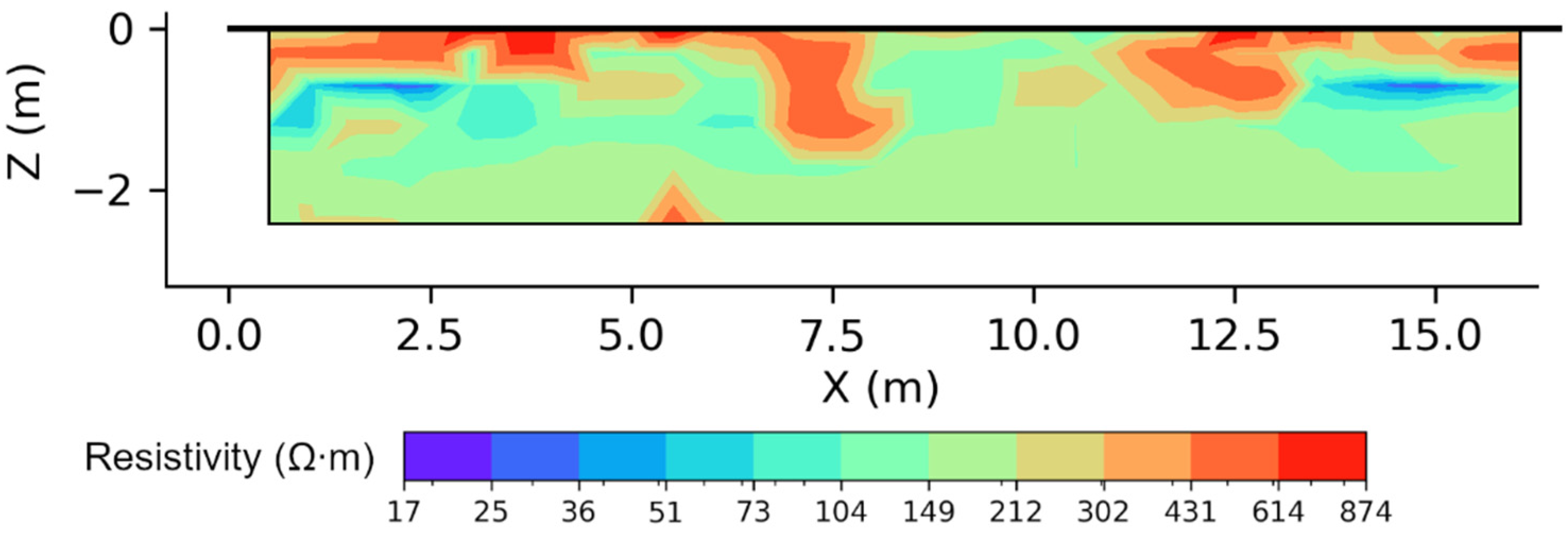
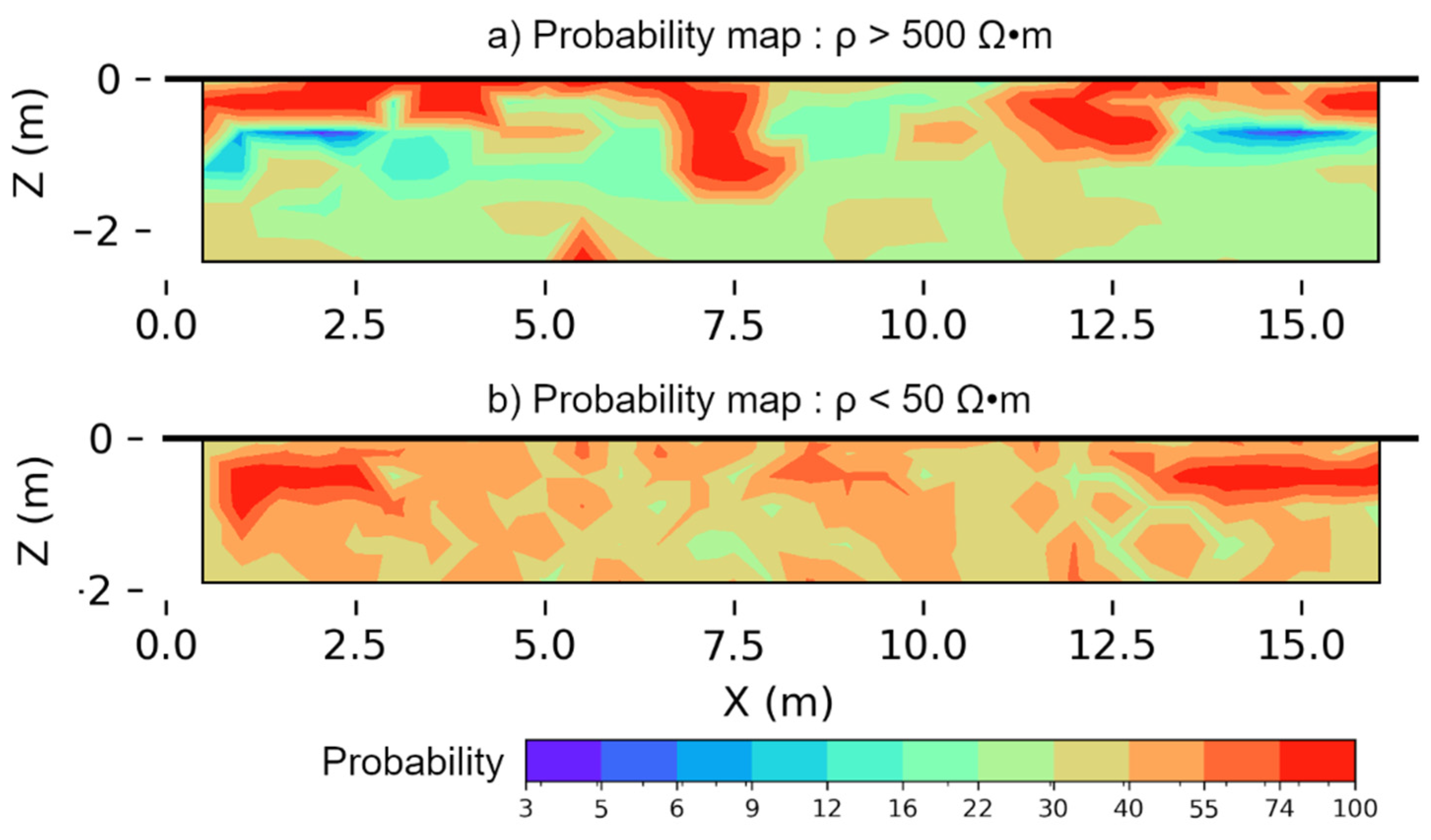
• The shadow part of the model (less than 0.6 m) is composed of the most resistant blocks. The average value of resistivity equals 300 Ω∙m and can reach 875 Ω∙m. A heterogeneity could be observed between 8 and 11 m, corresponding to an erosion part caused by the weathering of the stone.
• Under the shadow part, the resistivity values are stable, and the average value is 178 Ω∙m; however, between 6.5 and 8 m, an abnormally resistant area is identified, which corresponds to a mechanical fissure, verified by a geotechnical test.
• Two conductive layers are located on the left and right sides (between 0.5 to 2.5 m and 13 to 15.5 m). The average value of resistivity is 35 Ω∙m and the lowest value could attain 22 Ω∙m. This part could be the fissure filled with moisture, which caused the erosion of the wall.

The main purpose of the uncertainty analysis here is to verify whether the anomalies were artifacts of the inversion or true physical realities.

3.2. Model Sampling

The simulated ‘observation data set’ is generated from the inverted resistivity model. We chose to add 3% of white Gaussian noise to the data, according to the measurement quality factor. The family of rebuilt equivalent models is then illustrated by the uncertainty analysis. The comparison between the uncertainty analysis result and the real data inversion is presented. The model in Figure 2 is considered as the reference model in the following analysis.

To perform the model sampling procedure, the first step is the spectral decomposition via SVD (Equation (3)). According to Equations (3) and (4), the singular value of the reference model (Figure 2) and its cumulative information (Equation (4)) is shown in Figure 3. The singular values decrease fast with the augmentation of the index and, respectively, the cumulative information of the spectral increases with the index value. Moreover, the choice of basic terms quantity is in a range from 5 to 10, to avoid the difficulty of sampling the domain in a higher dimension. The latter will cause the concentration of the sampling points along the border of the research domain [39].

Figure 4 presents the five basic terms, calculated according to the inverted model. It is shown that the last two terms are barely the same, which is coincident with the fact that the cumulative information achieves a high level after the 4th singular value index. Each basic term represents a main scenario of resistivity. For instance, the basic term 1 corresponds mainly to the high value of resistivity, but in the 2nd term, the conductive zones on both the left and right sides of the model are highlighted.

3.3. Results of Uncertainty Analysis

The resistivity model and its interpretation are shown in Section 3.1. The inversion algorithm used is the least square with an L1-term optimization by an iterative re-weighted procedure. The difference between the real dataset and the inverted model is shown in Figure 5. It is observed that the difference between the real dataset and the prediction is not high. However, some peak values do appear at the locations of the current injection, which might cause misfits in the model.

The rebuilding of the sampling data is performed with Particle Swarm Optimization (PSO). This technique also uses an iterative approach to create a family of the equivalent models. Figure 6 shows the relative error curve with the increase in iterations. It is noted that the misfit will not monotonously decrease. However, the general trend of the relative error is to decline, showing that the PSO algorithm has the capacity to rebuild the equivalent model family. Furthermore, the relative error becomes lower than 10% after 10 iterations, which means it is possible to give an exploratory explanation of the data.

Figure 7 shows the probability map after the sampling procedure, which is a similar plot as shown in Figure 2. The results are similar. However, Figure 7a shows a simpler structure: the resistivity of the superficial part is superior to 500 Ω∙m, whose probability is close to 100%. Furthermore, the conductive anomaly at the left and right sides has very low probability of being in this interval. The central resistant anomaly seems to be connected to a lower part (about 2 m in depth).

There is a high probability that the conductive area between 0–2.5 m and 13–15.5 m is in the interval of resistivity ρ ⸦ [0, 50], as shown in Figure 7b. The geological interpretation in this area is confirmed by visual observation. The joints between the bricks are heavily weathered and filled with clayey moisture.

4. Discussion

The results show different steps performed to deduce the final equivalent model family. The cumulative information achieves 99.8% after four singular value indexes. According to the rule that the number of spectra should be between 5 and 10, we chose to perform the spectral decomposition for five basic terms. The PSO is then used to rebuild the equivalent model family. The samples in the equivalence family aim to deduce the indicator probability map, while the latter gives simpler structures of the same resistivity models.

The curve of relative errors (Figure 6) demonstrates that the optimization results become stable after about 10 iterations. That is the reason we chose the equivalent models obtained between 10 and 40 iterations to perform the uncertainty analysis by probabilistic approaches.

Another advantage of PSO can be observed in Figure 8. The dispersion rate is defined as the median of Euclidian distance between the particles in the research domain created by the algorithm. This rate of the 1st iteration is the coordinate of the center of gravity of the particle dispersion. It decreases to around 20% after three iterations and remains greater than 20%. It means that this algorithm has an explorative character in this study. Generally speaking, when the dispersion reaches under 5%, it is considered that the swarm during the optimization has collapsed in a unique direction. The last situation is not desired in the optimization algorithm because it could modify the posterior sampling strategies. Therefore, we constate that the optimization by PSO could equalize the exploration range and the convergence limit. Here, the swarm particle never converges to a local minimum so that the algorithm does not overfit the noise in the dataset.

Figure 9 shows two examples of the equivalent model family obtained by PSO. The differences between the family are classified by the k-means algorithm. The k-means clustering groups rebuilt equivalent models on their resistivity features. A user-defined number of clusters is predefined to divide the model family. Figure 9 illustrates that the structure of the two families is similar, but the resistivity range varies in different families. Moreover, the diffusion to the depth of the low-resistivity area is different, as the conductive area in family 2 is much larger than the one in family 1.

Mathematically, the linear uncertainty is calculated from the covariance matrix, according to [40]. A high value of uncertainty in Figure 10 indicates that the uncertainty value decreases with depth. Compared with the probability map (Figure 7), the high uncertainty also led to larger model variability. The linear uncertainty derived from the Jacobian matrix during the inversion is barely different from the actual uncertainty in a nonlinear inverse problem, encouraging the further study of nonlinear uncertainty analysis.

5. Conclusions

The objective of this paper was to develop a novel procedure to perform the uncertainty analysis over the inverse problem in ERT models. It is based on the dimension reduction by spectral decomposition through singular value decomposition. The posterior model sampling in the reduced basic terms is performed by the PSO algorithm. The variation in relative errors and dispersion demonstrate that this algorithm has the capacity to equalize the exploratory range and the convergence level. The uncertainty analysis is then performed on the whole set of equivalent models rebuilt by PSO, showing probabilistic maps of the resistivity in the inverted model, instead of the deterministic way.

The method is applied to real geo-electrical datasets of a wall fissure detection problem. With the intervention of the demonstrated approach, probabilistic maps are built with different segmentations of resistivities. The results have shown that in shadow depth, the conductive zone, on both the left and right side of the model, can be extensible. We assume that this reflects the possible extension of the moisture erosion inside the wall. Furthermore, the resistant area (superior to 500 Ω∙m), located in the deeper area, shows a slight extension, which may correspond to a developing fissure inside the wall. Compared with the existing state-of-the-art algorithm, the proposed method achieves better understanding of the ERT model. The probabilistic maps offer an enhanced interpretation of the possible development in the inverted model, reflecting the engineering reality.

In a real case, uncertainty means a misunderstanding of the inverted model. In nonlinear inversions, the uncertainty is composed of all the possible sources. The sources could be the choice of the optimal solution in the equivalent models, and the ambiguity from our geological or geotechnical knowledge. Therefore, the uncertainty analysis presented in this study serves to give other possible geotechnical interpretations in an engineering project. The future expansion of this study includes the use of different machine learning algorithms to perform the model sampling, aiming to find an approach with a better balance between accuracy and efficiency. It also concerns the expansion of the uncertainty analysis of other types of inversion problems.

References

1. Garrido, I.; Solla, M.; Lagüela, S.; Fernández, N. IRT and GPR Techniques for Moisture Detection and Characterisation in Buildings. Sensors 2020, 20, 6421. [Google Scholar] [CrossRef] [PubMed]
2. Vinha, J.; Salminen, M.; Salminen, K.; Kalamees, T.; Kurnitski, J.; Kiviste, M. Internal moisture excess of residential buildings in Finland. J. Build. Phys. 2018, 42, 239–258. [Google Scholar] [CrossRef]
3. Wang, X.; Liu, P.; Sun, Y.; Wang, W. Study on breaking concrete structures by pulse power technology. Buildings 2022, 12, 274. [Google Scholar] [CrossRef]
4. Ortega-Ramírez, J.; Bano, M.; Villa Alvarado, L.A.; Medellín Martínez, D.; Rivero-Chong, R.; Motolinía-Temol, C.L. High-resolution 3-D GPR applied in the diagnostic of the detachment and cracks in pre-Hispanic mural paintings at “Templo Rojo”, Cacaxtla, Tlaxcala, Mexico. J. Cult. Herit. 2021, 50, 61–72. [Google Scholar] [CrossRef]
5. Parracha, J.; Pereira, M.; Maurício, A.; Faria, P.; Lima, D.F.; Tenório, M.; Nunes, L. Assessment of the density loss in anobiid infested pine using X-ray micro-computed tomography. Buildings 2021, 11, 173. [Google Scholar] [CrossRef]
6. Civera, M.; Surace, C. Instantaneous spectral entropy: An application for the online monitoring of multi-storey frame structures. Buildings 2022, 12, 310. [Google Scholar] [CrossRef]
7. Garrido, I.; Barreira, E.; Almeida, R.M.S.F.; Lagüela, S. Introduction of active thermography and automatic defect segmentation in the thermographic inspection of specimens of ceramic tiling for building façades. Infrared Phys. Technol. 2022, 121, 104012. [Google Scholar] [CrossRef]
8. Tejedor, B.; Barreira, E.; Almeida, R.M.S.F.; Casals, M. Automated data-processing technique: 2D Map for identifying the distribution of the U-value in building elements by quantitative internal thermography. Autom. Constr. 2021, 122, 103478. [Google Scholar] [CrossRef]
9. Pang, G.; Wang, N.; Fang, H.; Liu, H.; Huang, F. Study of damage quantification of concrete drainage pipes based on point cloud segmentation and reconstruction. Buildings 2022, 12, 213. [Google Scholar] [CrossRef]
10. Munawar, H.S.; Ullah, F.; Shahzad, D.; Heravi, A.; Qayyum, S.; Akram, J. Civil infrastructure damage and corrosion detection: An application of machine learning. Buildings 2022, 12, 156. [Google Scholar] [CrossRef]
11. Stałowska, P.; Suchocki, C.; Rutkowska, M. Crack detection in building walls based on geometric and radiometric point cloud information. Autom. Constr. 2022, 134, 104065. [Google Scholar] [CrossRef]
12. Jeon, D.; Kim, M.K.; Jeong, Y.; Oh, J.E.; Moon, J.; Kim, D.J.; Yoon, S. High-accuracy rebar position detection using deep learning–based frequency-difference electrical resistance tomography. Autom. Constr. 2022, 135, 104116. [Google Scholar] [CrossRef]
13. Ren, H.; Tian, K.; Hong, S.; Dong, B.; Xing, F.; Qin, L. Visualized investigation of defect in cementitious materials with electrical resistance tomography. Constr. Build. Mater. 2019, 196, 428–436. [Google Scholar] [CrossRef]
14. Valero, L.R.; Sasso, V.F.; Vicioso, E.P. In situ assessment of superficial moisture condition in façades of historic building using non-destructive techniques. Case Stud. Constr. Mater. 2019, 10, e00228. [Google Scholar] [CrossRef]
15. Hola, A. Measuring of the moisture content in brick walls of historical buildings—The overview of methods. Presented at the IOP Conference Series: Materials Science and Engineering. 2017. Available online: https://iopscience.iop.org/article/10.1088/1757-899X/251/1/012067 (accessed on 31 March 2022).
16. Hoła, A. Methodology for the in situ testing of the moisture content of brick walls: An example of application. Archiv. Civ. Mech. Eng. 2020, 20, 114. [Google Scholar] [CrossRef]
17. Di Tommaso, A.; Cianfrone, F.; Pascale, G. Detection of internal fissures on rock structural elements of historical buildings. Eng. Fract. Mech. 1990, 35, 473–492. [Google Scholar] [CrossRef]
18. Xiong, Z.; Wang, Y.; Chen, X.; Xiong, W. Seismic behavior of underground station and surface building interaction system in earth fissure environment. Tunn. Undergr. Space Technol. 2021, 110, 103778. [Google Scholar] [CrossRef]
19. Kłosowski, G.; Rymarczyk, T.; Gola, A. Increasing the Reliability of Flood Embankments with Neural Imaging Method. Appl. Sci. 2018, 8, 1457. [Google Scholar] [CrossRef] [Green Version]
20. Verdet, C.; Sirieix, C.; Marache, A.; Riss, J.; Portais, J.-C. Detection of undercover karst features by geophysics (ERT) Lascaux cave hill. Geomorphology 2020, 360, 107177. [Google Scholar] [CrossRef]
21. Xu, S.; Sirieix, C.; Riss, J.; Malaurent, P. A clustering approach applied to time-lapse ERT interpretation—Case study of Lascaux cave. J. Appl. Geophys. 2017, 144, 115–124. [Google Scholar] [CrossRef]
22. Rymarczyk, T.; Kłosowski, G.; Hoła, A.; Hoła, J.; Sikora, J.; Tchórzewski, P.; Skowron, Ł. Historical buildings dampness analysis using electrical tomography and machine learning algorithms. Energies 2021, 14, 1307. [Google Scholar] [CrossRef]
23. Netto, L.G.; Filho, W.M.; Moreira, C.A.; Donato, F.T.; Helene, L.P.I. Delineation of necroleachate pathways using electrical resistivity tomography (ERT): Case study on a cemetery in Brazil. Environ. Chall. 2021, 5, 100344. [Google Scholar] [CrossRef]
24. Ray, A.; Sekar, A.; Hoversten, G.M.; Albertin, U. Frequency domain full waveform elastic inversion of marine seismic data from the Alba field using a Bayesian trans-dimensional algorithm. Geophys. J. Int. 2016, 205, 915–937. [Google Scholar] [CrossRef]
25. Carter, S.; Xie, X.; Zhou, L.; Yan, L. Hybrid Monte Carlo 1-D joint inversion of LOTEM and MT. J. Appl. Geophys. 2021, 194, 104424. [Google Scholar] [CrossRef]
26. Athens, N.D.; Caers, J.K. Gravity inversion for geothermal exploration with uncertainty quantification. Geothermics 2021, 97, 102230. [Google Scholar] [CrossRef]
27. Karolczuk, A.; Kurek, M. Fatigue life uncertainty prediction using the Monte Carlo and Latin hypercube sampling techniques under uniaxial and multiaxial cyclic loading. Int. J. Fatigue 2022, 160, 106867. [Google Scholar] [CrossRef]
28. Gnewuch, M.; Wnuk, M. Explicit error bounds for randomized Smolyak algorithms and an application to infinite-dimensional integration. J. Approx. Theory 2020, 251, 105342. [Google Scholar] [CrossRef] [Green Version]
29. Li, P.P.; Lu, Z.H.; Zhao, Y.G. An effective and efficient method for structural reliability considering the distributional parametric uncertainty. Appl. Math. Model. 2022, 106, 507–523. [Google Scholar] [CrossRef]
30. Liu, S.; Jia, J.; Zhang, Y.D.; Yang, Y. Image reconstruction in electrical impedance tomography based on structure-aware sparse Bayesian learning. IEEE Trans. Med. Imaging 2018, 37, 2090–2102. [Google Scholar] [CrossRef] [Green Version]
31. Rymarczyk, T.; Kłosowski, G.; Kozłowski, E. A non-destructive system based on electrical tomography and machine learning to analyze the moisture of buildings. Sensors 2018, 18, 2285. [Google Scholar] [CrossRef] [Green Version]
32. Rymarczyk, T.; Kłosowski, G.; Hoła, A.; Sikora, J.; Wołowiec, T.; Tchórzewski, P.; Skowron, S. Comparison of machine learning methods in electrical tomography for detecting moisture in building walls. Energies 2021, 14, 2777. [Google Scholar] [CrossRef]
33. Pidlisecky, A.; Knight, R. FW2_5D: A MATLAB 2.5-D electrical resistivity modeling code. Comput. Geosci. 2008, 34, 1645–1654. [Google Scholar] [CrossRef]
34. Tibshirani, R. Regression shrinkage and selection via the lasso. J. R. Stat. Soc. Ser. B (Methodol.) 1996, 58, 267–288. [Google Scholar] [CrossRef]
35. Günther, T.; Rücker, C.; Spitzer, K. Three-dimensional modelling and inversion of dc resistivity data incorporating topography—II. Inversion. Geophys. J. Int. 2006, 166, 506–517. [Google Scholar] [CrossRef] [Green Version]
36. Watkins, D.S. Fundamentals of Matrix Computations, 2nd ed.; Wiley-Interscience: New York, NY, USA, 2002. [Google Scholar]
37. Arboleda-Zapata, M.; Guillemoteau, J.; Tronicke, J. A comprehensive workflow to analyze ensembles of globally inverted 2D electrical resistivity models. J. Appl. Geophys. 2022, 196, 104512. [Google Scholar] [CrossRef]
38. Wolke, R.; Schwetlick, H. Iteratively reweighted least Squares: Algorithms, Convergence Analysis, and Numerical Comparisons. SIAM J. Sci. Stat. Comput. 1988, 9, 907–921. [Google Scholar] [CrossRef]
39. Fernández-Martínez, J.L.; Fernández-Muñiz, Z. The curse of dimensionality in inverse problems. J. Comput. Appl. Math. 2020, 369, 112571. [Google Scholar] [CrossRef]
40. Jafadideh, A.T.; Asl, B.M. A new data covariance matrix estimation for improving minimum variance brain source localization. Comput. Biol. Med. 2022, 143, 105324. [Google Scholar] [CrossRef]
Figure 1. Flowchart of the method used here to perform the uncertainty analysis.
Buildings 12 00622 g001
Figure 2. The inverted resistivity model, used as the reference model in the uncertainty analysis.
Buildings 12 00622 g002
Figure 3. The variation in the singular value obtained by Equation (3) (left axis) and the cumulative information of the spectral (right axis).
Buildings 12 00622 g003
Figure 4. Spectral basic terms of the resistivity model are shown in Figure 2. The color bar is on log10 scale, and the y-axis is the number of each layer.
Buildings 12 00622 g004
Figure 5. Difference between prediction (inversion) and the observation in log10 scale. Note that the peak value refers to the locations of current injections.
Buildings 12 00622 g005
Figure 6. Convergence Curve of PSO algorithm.
Buildings 12 00622 g006
Figure 7. Resistivity model in probabilistic view deduced from the uncertainty analysis of the rebuilt equivalent models: (a) ρ > 500 Ω∙m; (b) ρ < 50 Ω∙m.
Buildings 12 00622 g007
Figure 8. Dispersion rate with the iteration of PSO.
Buildings 12 00622 g008
Figure 9. Example of two different clusters of equivalent models obtained by k-means clustering. (a) family 1 from the 1st cluster; (b) family 2 from another cluster of the equivalent models.
Buildings 12 00622 g009
Figure 10. Linear uncertainty (in log scale) derived from the Jacobian matrix using the posterior covariance matrix.
Buildings 12 00622 g010
Publisher’s Note: MDPI stays neutral with regard to jurisdictional claims in published maps and institutional affiliations.