Gediminas Hill Slopes Behavior in 3D Finite Element Model

Abstract

In this manuscript, we present the results of three-dimensional finite element analyses performed in the cloud of a large-scale model of the Gediminas Hill buildings and the construction remains of the Upper and Lower castles in Vilnius city. The greatest challenge associated with the simulated numerical model is the difficult geological layer surface inclinations and soil–structure interaction behavior prognosis, which require significant computational resources. The purpose of this research work is to present current and possible worst-case scenarios for Gediminas Hill, considering its buildings and construction remains, regarding the stability of its slopes through a safety analysis. The construction of a numerical three-dimensional model of Gediminas Hill allows for us to assess the soil–structure interaction behavior. The results of non-linear analysis on the created model are in agreement with the tendencies observed in direct geodetic measurements and the relevant landslide history.

1. Introduction

Numerical modeling techniques have evolved with the improved use of computational resources. At first, two-dimensional (2D) numerical modeling was created, while three-dimensional (3D) numerical modeling was introduced later. Initially, when solving geotechnical problems by applying 3D modeling [1], only small-scale volumes with very limited finite element quantities or large-scale volumes with enormous finite elements could be used; in this regard, Kausel [2] has summarized the history of soil–structure interaction modeling very well. At present, 3D models are larger, more complex, and more computationally reliable [3,4,5,6]. The progress of high-performance calculation methods has allowed for the performance of stochastic finite element analyses using large-scale meshes or a large amount of Monte Carlo simulations [7,8].

Three-dimensional geotechnical models are more suitable for large projects [9]. When such projects are analyzed, it is easier to spend more time on 3D numerical model preparation and obtain the results at any necessary area or point than to conduct many 2D calculations in different cross-sections and obtain results that are only valid in the chosen 2D simulation cross-section. Furthermore, in 2D slope stability analysis, the landslide width cannot be obtained. This is why 3D finite element modeling is very important for slope stability analysis [10]. Additionally, 3D geotechnical modelling can help to define representative borehole logs indicating the stratification of soil [11], the geometry of different sedimentary layers [12], and whether it is necessary to add the superstructure to the model [13]. The 3D geotechnical model can help to determine the weakest areas in the model by analyzing the reduction in safety [14].

One of the most interesting and actual objects—from a geotechnical and geological engineering point of view—in Lithuania, to which a 3D model can be applied, is Gediminas Hill and the remains of its Upper castle in Vilnius city. This object is very important to the local community, as it is included in the Lithuanian culture heritage register. Various studies on Gediminas Hill have already been carried out [15,16,17,18,19,20,21,22,23]. The purpose of this research is to present the current and possible worst-case scenarios of Gediminas Hill and the remains of the Upper castle, regarding the stability of slopes, by conducting a factor of safety analysis. The reliability of the 3D geotechnical model is ensured by validating obtained results with respect to the existing monitoring data.

2. Input Data

This section introduces the initial data entered into the 3D model, which consisted of geological engineering and geotechnical conditions; the geodetic surface; building remains and structure plans; pedestrian pathways; and tunnels. All these data were prepared for entry into 3D model, which was calculated using a VILNIUS TECH virtual computer.

2.1. Computational Resources

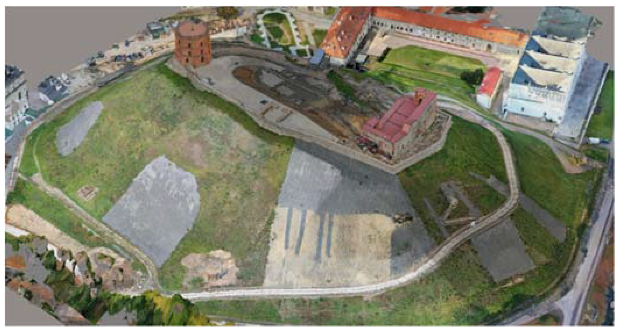
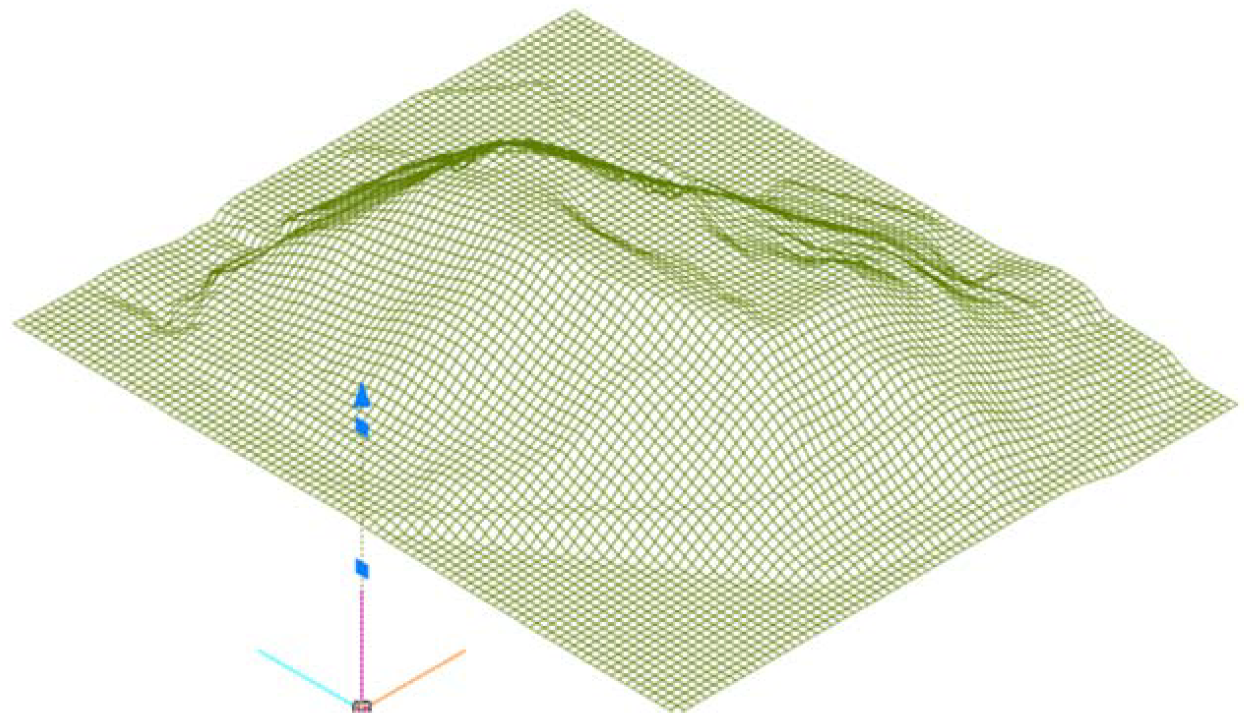
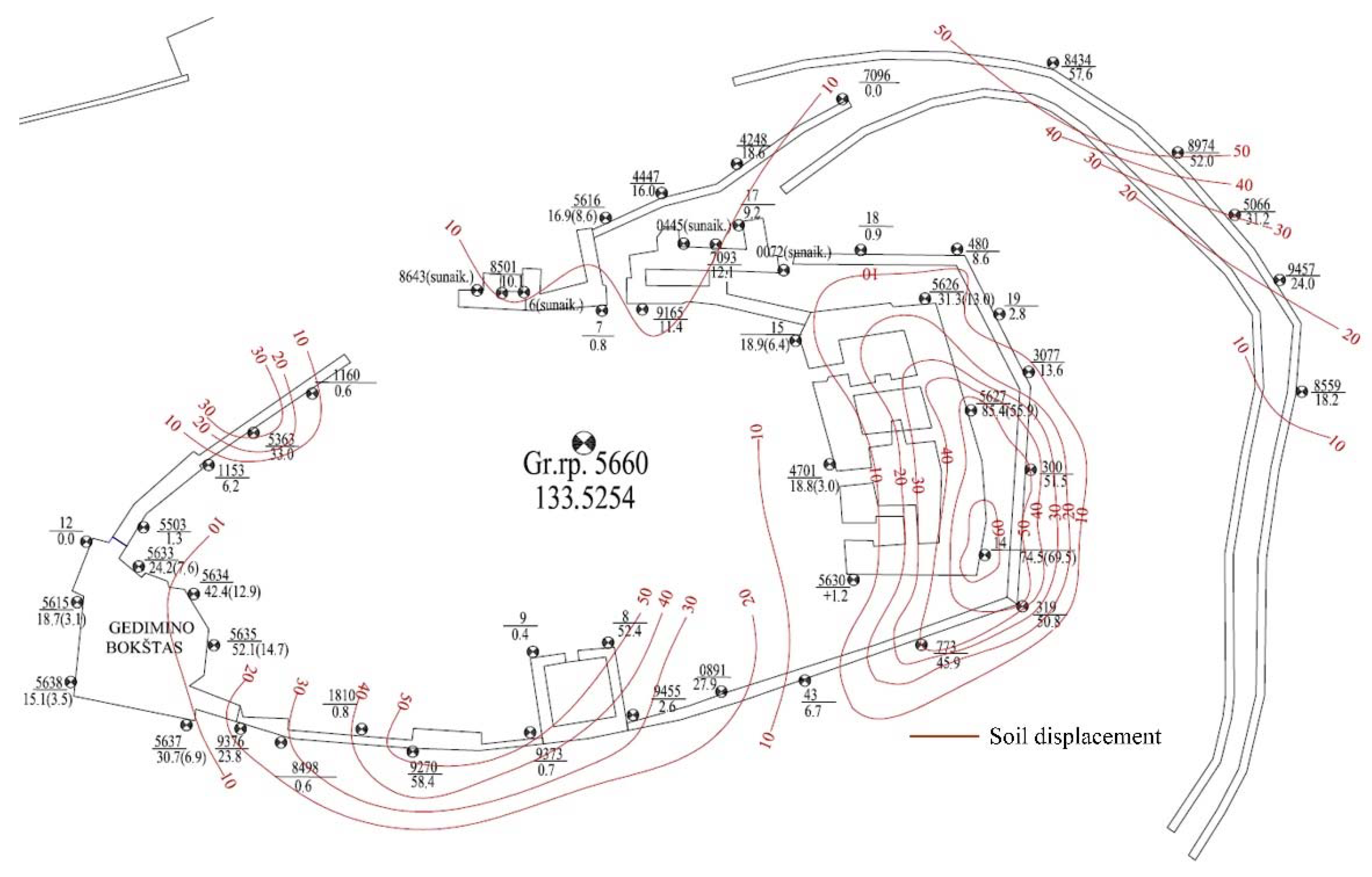
The numerical modeling was simulated in a private VILNIUS TECH cloud. Cloud services were chosen to quickly respond to the changing needs of the computing resource. This was the first time that such large-scale calculations were performed using the university’s private computing resources, making it difficult to determine the associated resource needs. A physical server was prepared in the VILNIUS TECH data center for these calculations, which was connected to the VILNIUS TECH private cloud. The cloud service uses open-source OpenStack software that allows for the construction of private clouds. The physical server has 2 Intel Xeon Gold 5220R 2.2 GHz processor units, 1536 GB RAM, and uses 6 TB space, which was combined from 8 SSD drives. For the first calculations with the virtual server, 20 core CPU resources and 320 GB of RAM were assigned; however, the calculation capacity was later increased to 1015 GB RAM. To ensure successful numerical simulations with the DIANA finite element analysis (FEA) release 10.3 [24], the virtual server was connected to the department of Information systems resource monitoring system, which allowed for the server loads to be monitored and faults in the numerical simulation to be quickly identified.

2.2. Geodetic Data

The investigated surface of the Gediminas Hill area was scanned and a 3D surface model was created from simple photographs using the Acute3D Viewer [25] software. To ensure the high resolution of the 3D surface model, photogrammetry, computer vision, and computational geometry algorithms were used, fulfilling industrial quality requirements in terms of precision, scalability, efficiency, usage, robustness, and interoperability. A general view of the Gediminas Hill 3D surface is presented in Figure 1.

The generated geodetic model point cloud was very dense and not suitable for 3D modelling. It was necessary to prepare simplifications of the geodetic data, as follows: for slopes and pedestrian pathways, the surface point density must be no less than 0.5 m, and the construction surface density must be no less than 0.2 m. Furthermore, it was very important to know where the construction edge ends and the soil starts; therefore, the contact points of different objects also were included into the geodetic surface model. According to accepted simplifications of the geodetic data, a three-dimensional surface of Gediminas Hill was created (Figure 2).

2.3. Engineering Geological and Geotechnical Conditions

From a geomorphological perspective, Gediminas Hill is located on the north-western edge of the Medininkai Highland, part of the Ašmena Upland, formed during the Middle Pleistocene Glaciation [26]. According to [27], the geological structure of the Gediminas Hill is represented by deposits from a few Pleistocene glaciations and, according to the Quaternary period stratigraphic scheme currently approved for use in the Lithuanian Geological Survey, the deposits depend on Dainava (Elsterian 2) and Žeimena formations of the Middle Pleistocene [28]. The Žeimena Formation can be subdivided into deposits of the Žemaitija (Saalian) and Medininkai (Warthian) sub-formations. The Middle Pleistocene deposits are affected by deluvial processes and human activities on the surface and slopes of the hill [27].

The last major engineering geological and geotechnical investigations of Gediminas Hill were carried out in 2019 and 2020 [29]. Detailed hydrogeological conditions of the site have been presented by [27]. During these investigations, geological engineering layers, along with their physical and mechanical properties, were identified (

Table 1. Summary of physical and mechanical properties of Gediminas Hill [27,29].

Stratigraphy Index	Soil Layer Identification	Soil Type	γ, kN/m3	ρ, Mg/m3	ρs, Mg/m3	w, %	wP, %	wL, %	k, m/d	φ’ (Degrees)	c’, kPa	cu, kPa	E, 1 MPa
tIV-dIV	tIV	Sa; Si;Cl	17.76	1.81	2.67	9.7	13.4	16.9	1.94	35.3	13.5	-	3.6
gdIImd	31	Cl	21.49	2.19	2.69	12.1	11.0	20.3	-	-	-	71.0	21.4
	32		21.76	2.22	2.69	11.4	12.1	19.9	-	33.8	15.3	-	33.1
	33		22.30	2.27	2.69	11.0	12.1	21.7	-	32.4	48.8	-	93.2
	34		20.51	2.09	2.69	10.3	12.8	18.2	-	44.6	21.1	-	7.3
fIImd	41	Sa	17.46	1.78	2.66	3.7	-	-	8.94	31.6	24.0	-	30.8
	42		19.02	1.94	2.66	10.7	-	-	7.35	38.1	34.1	-	56.8
	43		19.85	2.02	2.67	14.4	-	-	5.91	36.7	36.7	-	96.9
	44		16.56	1.69	2.66	3.2	-	-	12.1	32.8	11.5	-	-
lgIIžm	51		20.12	2.05	2.68	14.9	14.4	18.0	0.11	35.8	30.2	-	79.2
	52	Cl-Si	21.16	2.16	2.68	14.3	14.6	19.9	-	35.1	46.2	-	110.7
	53	Cl	20.09	2.05	2.72	21.2	20.9	38.9	-	14.5	107.0	-	79.9
	54	Sa	20.15	2.05	2.67	15.3	-	-	4.9	39.2	40.9	-	112.0
gdIIžm	61	Cl	22.11	2.24	2.69	11.5	22.0	12.2	-	28.1	76.9	-	74.2
	62		21.78	2.22	2.69	10.9	21.0	10.8	-	-	-	115.0	29.0
	63		21.59	2.20	2.69	15.0	25.8	13.0	-	-	-	81.6	17.5
	64		21.39	2.18	2.70	14.8	26.4	12.2	-	-	-	28.8	6.2
lgIIdn	71	Sa	19.71	2.01	2.67	16.5	19.9	15.7	0.39	37.5	41.7	-	119.9
	72	Si	20.00	2.04	2.68	15.7	20.0	15.8	0.08	33.1	73.1	-	186.1
	73	Sa	17.19	1.75	2.66	3.3	-	-	1.56	30.4	29.0	-	-
	74	Sa	19.86	2.03	2.67	15.7	-	-	1.68	36.9	37.4	-	139.2

¹ Note: E—calculated according to cone penetration tests with pore pressure (q_t) results; γ—unit weight; ρ—density; ρ_s—particle density; w—natural water content; w_P—plastic limit water content; w_L—liquid limit water content; k—coefficient of permeability; φ’—effective angle of internal friction; c’—effective cohesion; c_u—undrained cohesion; E—Young’s modulus.

).

Seeking to simplify the 3D geotechnical model, the geological layers given in Table 1 were formed by joining some layers with the same stratigraphy index; that is, some geological layers were averaged in height and their properties were determined based on existing local geotechnical experience. The simplified geological layer properties used in the 3D geotechnical model are given in

Table 2. Geological engineering layer properties used in the 3D model.

Stratigraphy Index	Soil Name 1	E, MPa	ν	ρ, t/m3	e	c, kPa	φ’ (Degrees)	Ψ (Degrees)
tIV-dIV	Mg	3.6	0.30	1.81 2.04 **	0.61	13.5	35.3	0.0
gdIImd	saCIL	33.1	0.35	2.22	0.35	15.3	33.8	3.0
fIImd	Sa	56.8	0.30	1.94	0.53	34.1	38.1	8.0
gdIImd	saCIL	33.1	0.35	2.22	0.35	15.3	33.8	3.0
lgIIžm	siSa	110.7	0.35	2.16	0.43	46.2	35.1	5.0
lgIIžm	saCIL-SiL	79.2	0.35	2.05	0.49	30.2	35.8	6.0
gdIIžm	saCIL	74.2	0.35	2. 24	0.34	76.9	28.1	2.0
lgIIdn	siSa	119.9	0.30	2.01	0.55	41.7	37.5	7.5
tIV ***	siSaW	12.0	0.35	1.74	0.65	12.3	35.8	0.1

¹ Soil name assigned according to EN ISO 14688-1:2018 [32]; ** saturated density; *** tunnel backfill properties; E—Young’s modulus; ν—Poisson’s ratio; ρ—density; c—cohesion; φ’—angle of internal friction; Ψ—dilation angle.

. The dilatancy angle (Table 2) was also accepted, according to [30], where the dilatancy of clay (except for over-consolidated clay) is mostly ψ ≈ 0°, while the dilatancy of sand depends on both the density and the angle of internal friction, and can be found using the equation ψ ≈ ϕ − 30° [31].

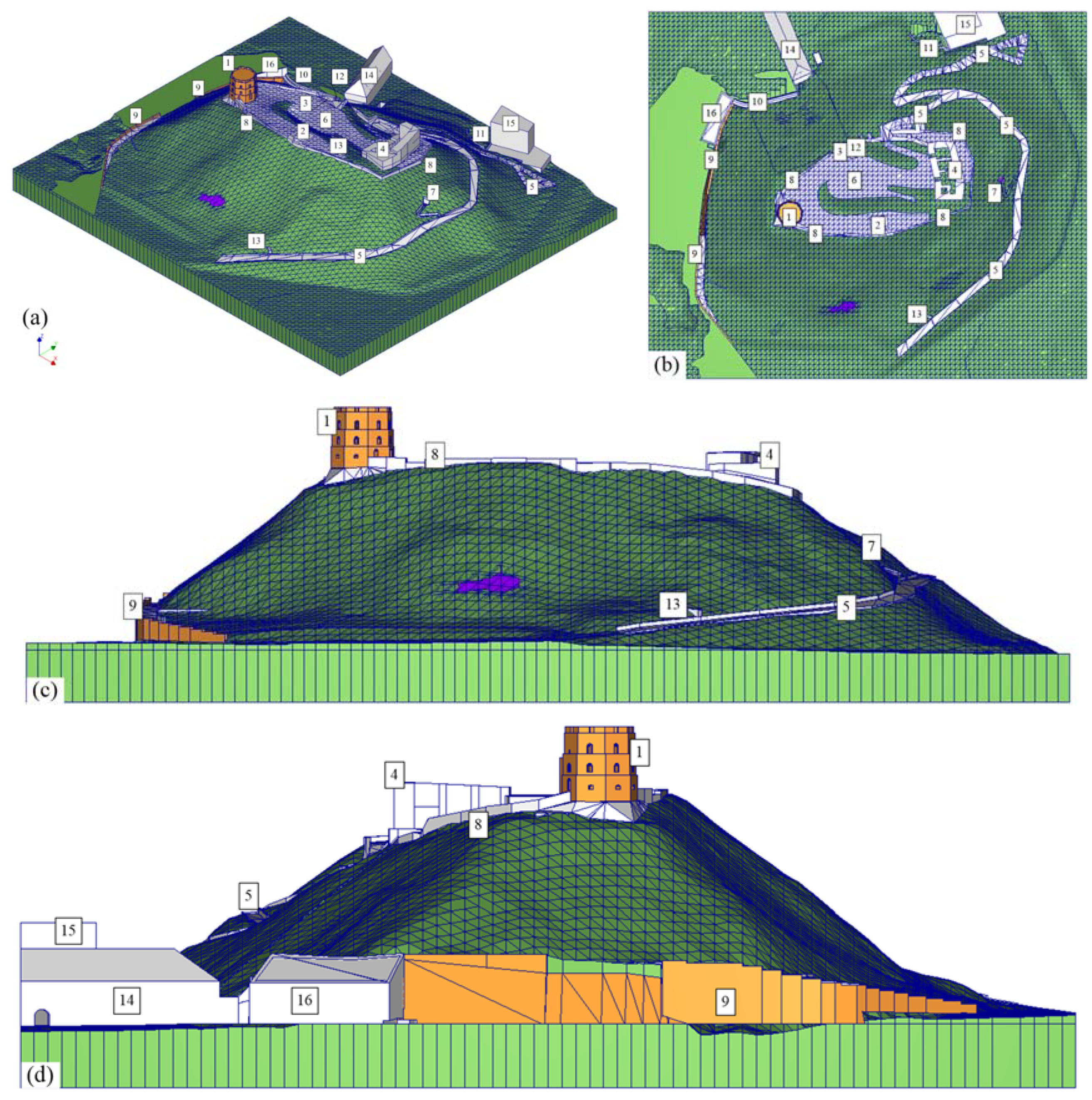
2.4. Buildings and Structures Remains, Path, Funicular and Tunnels

Ten construction remains objects, a pedestrian path, two tunnels, and one funicular are situated in the area of Gediminas Hill (Figure 3). All the buildings and construction remains were included in the numerical 3D model. The top of Gediminas Hill can be reached by a pedestrian pathway or funicular (Figure 3). At present, visitors are not allowed to see the tunnels, which were installed during World War I and World War II. One tunnel was excavated vertically from the top of Gediminas Hill (depth ~37–40 m) and has two exit ways (to the south-western and north-western slopes). The south-western tunnel length is ~88 m and the north-western tunnel length is ~79 m. This tunnel, due to its age and the rotten timber construction damages that occurred in 1960 [33], was filled with a liquid sand mixture to avoid tunnel construction failure. Another tunnel, which is close to the castle-keeper’s building [34], is quite short (~13 m), but has not been filled with liquid sand mixture. It is worth noting that this tunnel was only found at the end of 2019, at which point its timber construction was in a very bad condition; therefore, during 2020, bearing construction reconstruction of this tunnel was carried out.

3. Development of a Numerical Three-Dimensional Model of Gediminas Hill

According to the existing investigations of Gediminas Hill buildings and structure remains, as well as slope-monitoring, it was observed that shallow landslides form on the slopes. For this reason, in 3D numerical simulations, the Mohr–Coulomb material model was accepted for soil, while linear constitutive material models were used for buildings and remains. After analysis, the relevant literature, existing drawings, and information sources, and the geometry and locations of certain objects, were determined, and a three-dimensional numerical model of Gediminas Hill was created. The dimensions of the numerical model were 270 m in the east–west direction and 228 m in the south–north direction. The height of the model—from the horizontal supporting plane to the top of the west tower—was 76.47 m. The distance from the ground surface to the horizontal plane at different angles of the model varied from 7.9 m to 15.4 m. The lower horizontal plane of the numerical model (as well as the lateral surrounding surfaces) was constrained in all directions. In total, 1,847,241 finite elements were used, the size of which was not constant.

A numerical model of Gediminas Hill, comprising the soil layers forming the mountain, as well as the buildings and structures placed on it (Figure 3), was created in the finite element program Diana 10.3. The hill array consisted of eight major soil layers (Table 2), classified as solid volumetric bodies. Surfaces were used to separate the soil layers, which were composed of 3D Face-type elements interconnected in three-dimensional (x, y, z) space (as in Figure 2). The approximate dimension of one 3D Face element was 3.0 × 3.0 m. The three-dimensional face surfaces and their nodes, created in the drawing program, were localized using the Lithuanian coordinate system 94 (LKS94) coordinate system, and the heights were in correspondence with the Lithuanian elevation system (LAS) system.

The behavior of the numerical model and slope stability were determined through a four-stage calculation analysis. All four stages were assigned to three phases. In the first stage, the self-weight of the natural soil layers and tunnel backfill were evaluated (Figure 4, Phase 1). In the second stage (Figure 4, Phase 2), the self-weight of the technogenic soil layer (tIV-dIV) and gabions in the northern slope part (

Table 3. Additional properties for Gediminas Hill north slope.

Layer	E, MPa	ν	ρ, t/m3	e	c, kPa	φ’, (Degrees)	Ψ, (Degrees)
Gabions surrounding soil	40	0.33	1.85	0.6	2	39.98	9.99
Gabions	120	0.22	2.50	0.6	5	44.98	14.99

E—Young’s modulus; ν—Poisson’s ratio; ρ—density; e—porosity; c—cohesion; φ’—angle of internal friction; Ψ—dilation angle.

) were evaluated. The gabions were installed on natural soil layers to replace technogenic soil due to the occurrence of a shallow landslide in 2016 [18]. The third stage (Figure 4, Phase 3) involved evaluating the construction and self-weight of buildings, as well as additional loads on the pedestrian pathway (Figure 3) and the remains of the Upper castle pitch (Figure 3). In the fourth stage (Figure 4, Phase 3), slope stability calculations assessing the reduction in the strength of the technogenic soil layer saturation were initiated [35].

A non-linear numerical analysis of slopes displacements was conducted using different material models for soils, structures, and building remains. For the soil layers, the Mohr–Coulomb plasticity material model was applied, the properties of which are given in Table 2 and Table 3. Additional properties are given in Table 3, detailing the properties of the accepted gabions and gabions surrounding soil in the northern slope.

For the simulated constructions and building remains, elastic body mechanical properties were assigned, which represent the behavior of stone masonry and bricks up to their plastic limits. Structures and buildings transferred loads to the soil layers. The mechanical properties of the evaluated structures and building remains are presented in

Table 4. Properties of structures and buildings remains.

Element	E, MPa	ν	ρ, t/m3
Remains of Upper castle pitch (Figure 3)	1300	0.2	2.5
Pedestrian path (Figure 3)	1300	0.2	2.5
Rest of all construction remains (Figure 3)	2600	0.2	2.9
Remains of Old Arsenal (Figure 3)	2600	0.2	0.532

E—Young’s modulus; ν—Poisson’s ratio; ρ—density.

. The remains of the Old Arsenal building were simulated with low density (Table 4), as the construction of this building was not investigated by the authors; therefore, the volume of internal spaces was evaluated to reduce the total masonry density.

Before conducting the numerical simulation stages and phases (Figure 4), the numerical model must be filled with volumetric finite elements. All the finite element volumes were divided into hexa/quad-type elements, where, for total element volume coverage, tetrahedral/triangle-type elements can additionally be used. The size of a finite element depends on the meshed volumetric body edge length, as the length is divided into two parts. If the division number is increased, the required computational resource quantity automatically increases; thus, it is necessary to evaluate the capacity of computational resources based on the difficulty associated with the simulated geometry. The calculation time also depends on the quantity of the finite elements.

In the third calculation phase (Figure 4), all volumetric finite elements are active. When the self-weight evaluation reaches 100% in the third phase, strength reduction analysis is only initiated for the tIV-dIV soil layer. For other layers, the reduction in safety is not assessed.

The strength reduction method (SRF), sometimes referred to as the strength reduction finite element method [36], is a technique for calculating the slope factor of safety (FoS) [37], defined as the ratio of current soil shear strength to the minimum shear strength necessary to avoid failure. Alternatively, the FoS is considered as the factor required to reduce the soil strength to produce imminent failure. In SRF, the strength characteristics of the soil materials (cohesion and tangent angle of internal friction) are reduced by a factor until the loss of stability or failure of the structure occurs, as follows [38,39]:

$$F{S}_{n+1}=F{S}_n+\mathsf{\Delta }FS.$$

(1)

If the factor of safety calculated by Formula (1) does not converge, then a new lower increment is evaluated to obtain a new factor of safety, which reaches convergence:

$$\mathsf{\Delta }FS=\frac{\mathsf{\Delta }FS}{2}.$$

(2)

If this is not converged after the application of Formula (2), then the results are evaluated using the last convergence factor:

$$F{S}_{n+1}=F{S}_n.$$

(3)

At first, the strength reduction analysis factor of safety is equal to 1.0:

$$F{S}_n=F{S}_0=1.0.$$

(4)

With each chosen factor, the soil cohesion (5) and tangent angle of internal friction are reduced (6):

$$c_{n+1}=\frac{c}{F{S}_{n+1}},$$

(5)

$$\tan {\phi }_{n+1}=\frac{\tan {\phi }_n}{F{S}_{n+1}}$$

(6)

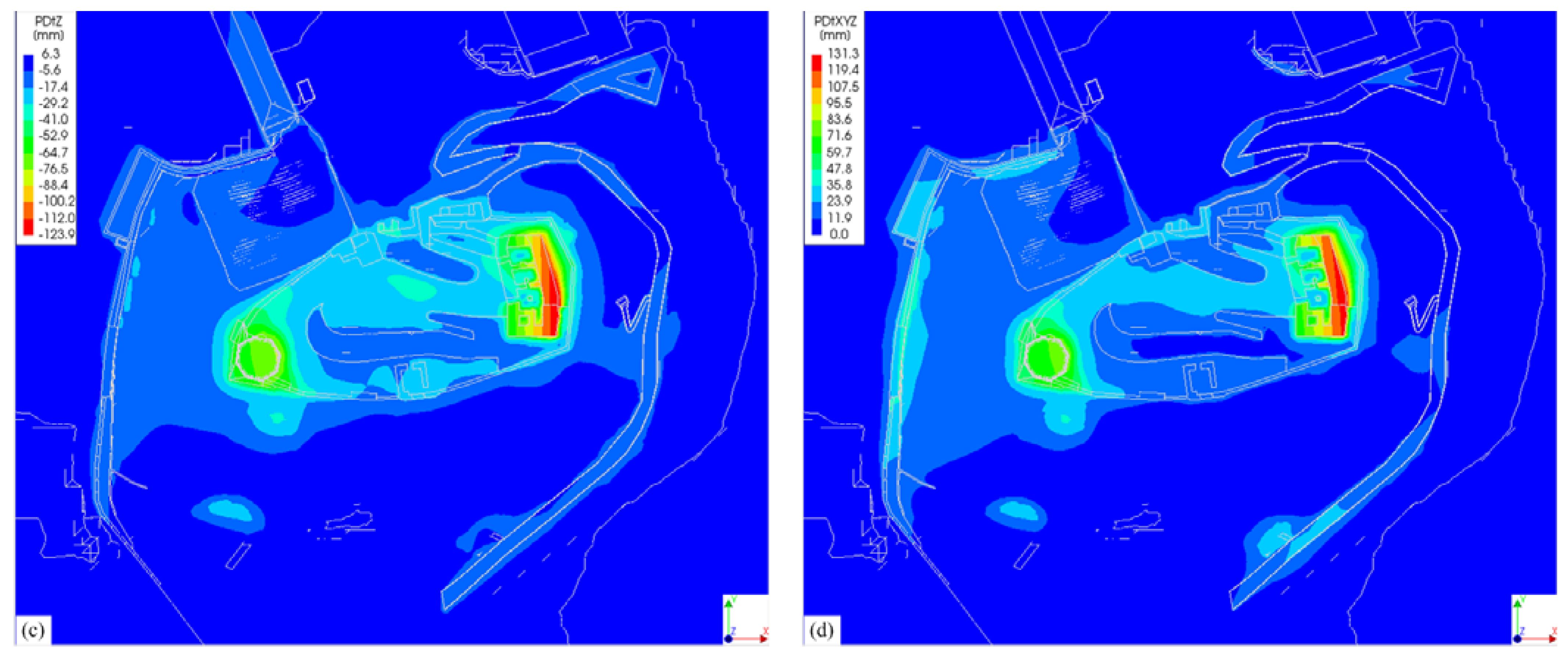
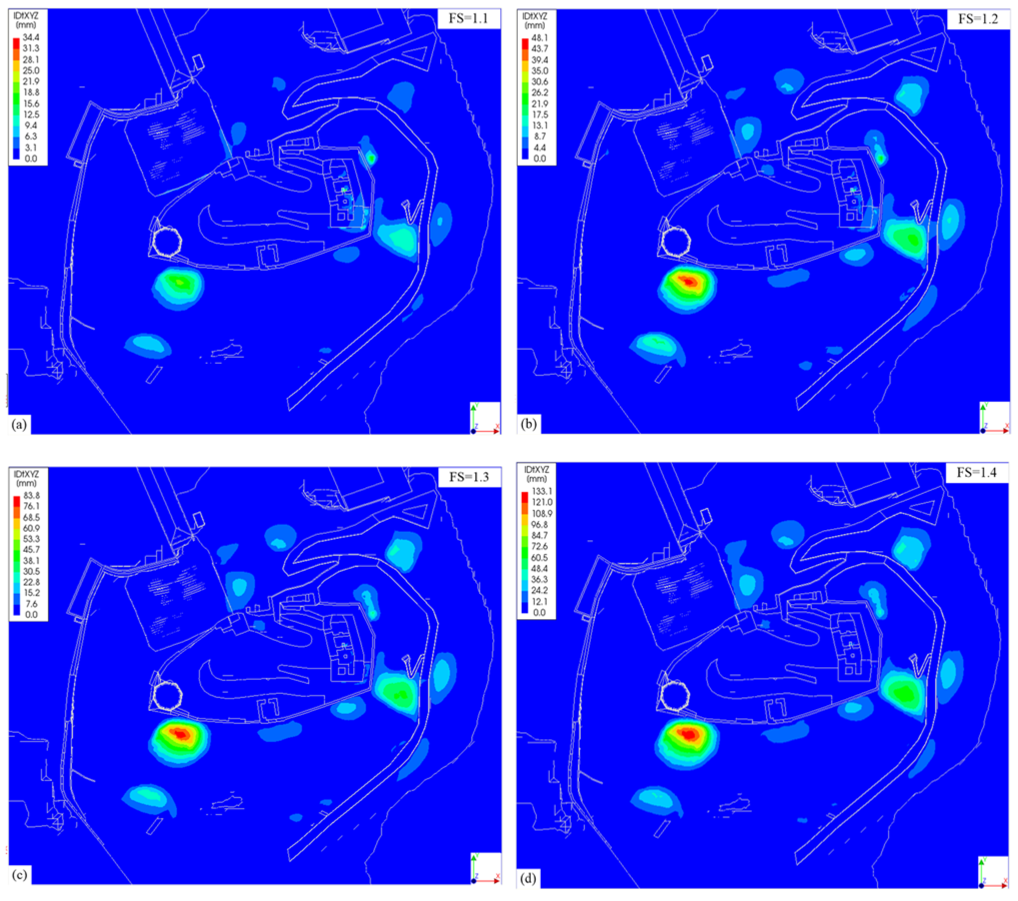
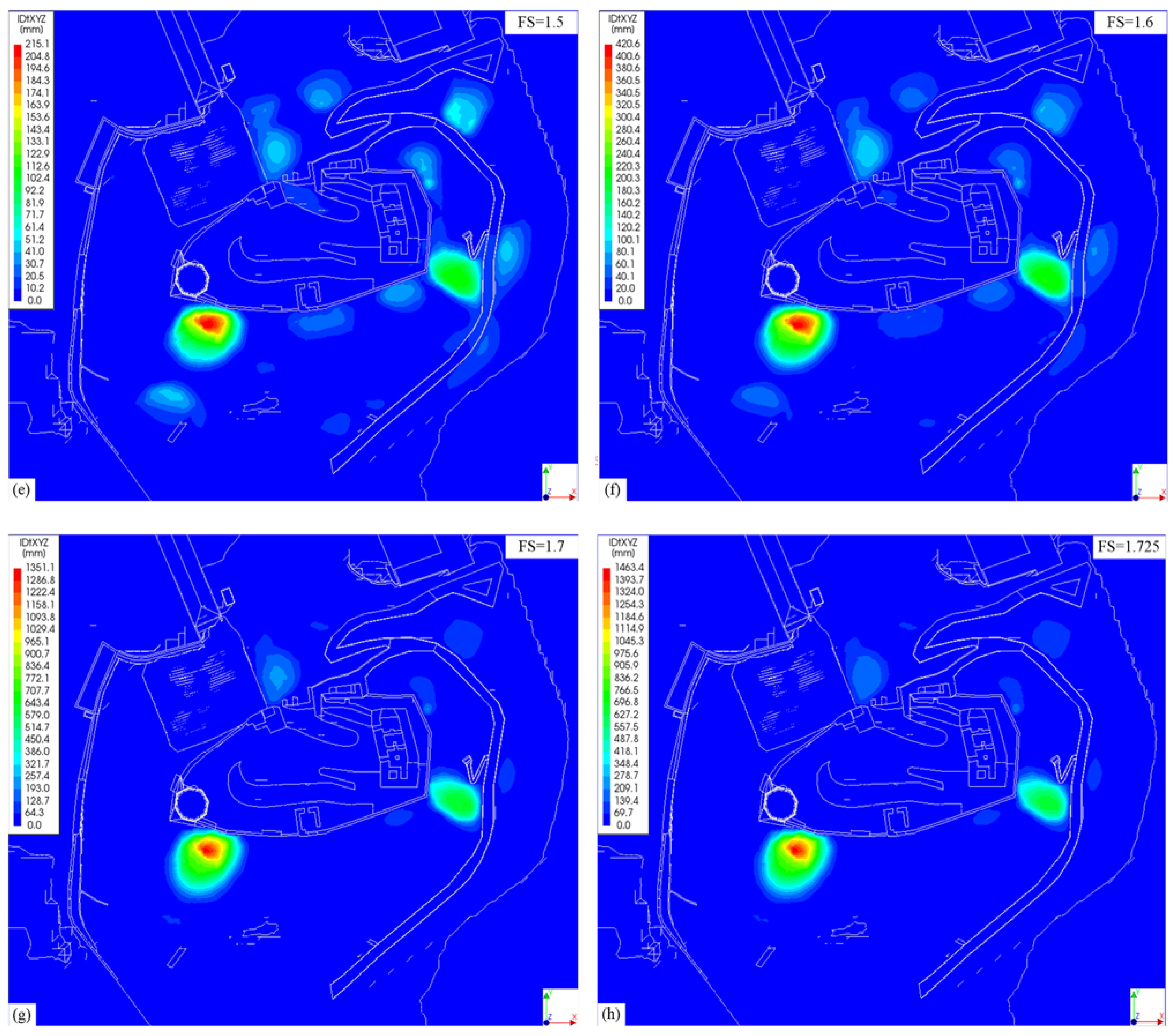
4. Behavior of Numerical Model

The interaction behavior of finite elements in a numerical model depends on their physical and mechanical properties, material models, supports or loads, finite element size and quantity [40], and slope width [41], among other factors. Historically, the behavior of Gediminas Hill has depended on additional factors, including climate change and the history of landslides [33]. All these factors increase the required computational resources. The considered model of Gediminas Hill demanded a calculation capacity of up to 1015 GB RAM. Processing such a numerical model can take from 25 to 26 h, of which from 4 to 5 h are required for the generation of the finite element mesh and from 20 to 22 h for numerical analysis. The finite element generation time depends on the complexity of the model geometry and the set of mesh parameters. The numerical analysis time also depends on the number of finite elements that are generated and the development of displacements. If larger displacements occur, the calculation process requires more iterations and, with each safety analysis step, the number of iterations increases. Therefore, the numerical analysis in the third phase took the longest. The obtained results on slope displacements from the third simulation phase without a strength reduction analysis (Figure 4) are presented in Figure 5.

The displacements presented in Figure 5 showed the same tendency as the monitoring data (presented in Figure 6). Thus, the compiled 3D numerical model can present the same slope movement tendencies. It is very problematic to obtain authentic results when historic object behavior is simulated, as the buildings in the model were built of bricks and stones in 1419, partially demolished in 1655–1661, restored and conserved in 1816–1817, 1930–1939, and 1956–1963, and conserved and partially restored in 1990–1993 [42]. Thus, the biggest concentration of soil displacements was close to the remains of the Upper castle western tower and the Upper castle remains (Figure 5). Seeking to develop a prognosis for the possible formation of landslide areas, strength reduction calculations were carried out in the third simulation phase (Figure 4). The strength reduction analysis was applied only to the tIV-dIV soil layer (Table 2), as existing knowledge and monitoring data [43] have shown that landslides only form in the tIV-dIV layer. These landslides are shallow.

Strength reduction analysis of the technogenic soil (tIV-dIV) layer (Figure 7) allowed for us to determine areas with the highest concentrations of displacements. Strength reduction analysis indicated not only displacements of the technogenic soil layer (tIV-dIV), but also displacements of constructions and buildings (in some places, the technogenic soil layer is under the foundations). In each SRF calculation, the depth of the technogenic soil (tIV-dIV) layer is different due to the soil displacements, where the newly formed soil mass is evaluated. When shallow landslides form, they include only technogenic soil (tIV-dIV). The increasing mass and volume of the moving soil causes stability failure, and a local shallow landslide occurs.

According to Figure 7, the highest possibility of shallow landslide formation was observed in the eastern and south-western slopes. The formation of these landslides correlates with tIV-dIV soil layer thickness—a thicker layer increases the landslide possibility and vice versa. A shallow landslide in the eastern slope occurred on 07 February 2022 (Figure 8), which appeared under the most difficult environmental conditions: the top layer of the soil was not frozen, and there was a lot of melting water under snow cover.

In Figure 8, the assigned tags correspond to those given in Figure 3. The landslide location and size (width, 6–6.5 m; length, 11–11.5 m) correlated well with the displacement zone obtained in the numerical simulation (Figure 7).

5. Conclusions

To create a volumetric numerical model of Gediminas Hill, it was necessary to utilize various recent and historical data. The constructed numerical model allowed for us to evaluate the slope stability behavior of Gediminas Hill, based on the accepted material models, loads, calculation phases, and so on, from which we drew the following conclusions:

• Constructions, buildings, and additional loads increased soil displacement, mostly in the technogenic (tIV-dIV) soil layer. The analyzed monitoring data, including recent and historical investigation reports on the constructions, as well as the numerical model behavior, allowed us to assume that the deformation of building remains depends on technogenic (tIV-dIV) soil layer displacements. The influence of the climate (i.e., precipitation) on slope stability was also evaluated, considering strength reductions, which demonstrated that the slope stability depends on the technogenic soil layer height and the inclination of undisturbed soil layers.
• The surface inclination of natural soil layers at the point of contact with the technogenic (tIV-dIV) soil layer in some areas is higher than that of the technogenic soil layers. In these areas, the biggest deformation zones may form. Numerical model analysis allowed for us to make the conclusion that technogenic (tIV-dIV) soil layer shallow landslide occurrence depends on the layer height, changes in mechanical parameters, and the surface inclination of the natural soil layers.
• The numerical Gediminas Hill 3D model allowed for us to assess the soil–building interaction behaviors. The results of non-linear analysis of the created model corresponded to the tendencies observed in direct geodetic measurements and were in agreement with the relevant landslide history.

References

1. Hovland, H.J. Three-Dimensional Slope Stability Analysis Method. J. Geotech. Eng. Div. 1977, 103, 971–986. [Google Scholar] [CrossRef]
2. Kausel, E. Early History of Soil–Structure Interaction. Soil Dyn. Earthq. Eng. 2010, 30, 822–832. [Google Scholar] [CrossRef] [Green Version]
3. Khan, M.S.; Park, J.; Seo, J. Geotechnical Property Modeling and Construction Safety Zoning Based on GIS and BIM Integration. Appl. Sci. 2021, 11, 4004. [Google Scholar] [CrossRef]
4. Weir, F.; Fowler, M.; Sullivan, T.; Kobler, M.; Bu, J. Evolution of a Geotechnical Model for Slope Design in an Active Volcanic Environment. In Proceedings of the 2020 International Symposium on Slope Stability in Open Pit Mining and Civil Engineering, Australian Centre for Geomechanics, Perth, Australia, 12–14 May 2022; pp. 455–472. [Google Scholar]
5. Andersen, T.R.; Poulsen, S.E.; Pagola, M.A.; Medhus, A.B. Geophysical Mapping and 3D Geological Modelling to Support Urban Planning: A Case Study from Vejle, Denmark. J. Appl. Geophys. 2020, 180, 104130. [Google Scholar] [CrossRef]
6. Zhang, G.; Zhu, J.; Chen, C.; Tang, R.; Zhu, S.; Luo, X. Analytical Reliability Evaluation Framework of Three-Dimensional Engineering Slopes. Buildings 2022, 12, 268. [Google Scholar] [CrossRef]
7. Savvides, A.A.; Papadrakakis, M. A Computational Study on the Uncertainty Quantification of Failure of Clays with a Modified Cam-Clay Yield Criterion. SN Appl. Sci. 2021, 3, 1–26. [Google Scholar] [CrossRef]
8. Wang, M.-Y.; Liu, Y.; Ding, Y.-N.; Yi, B.-L. Probabilistic Stability Analyses of Multi-Stage Soil Slopes by Bivariate Random Fields and Finite Element Methods. Comput. Geotech. 2020, 122, 103529. [Google Scholar] [CrossRef]
9. Aery, B. Recent Advances in Geotechnical Infrastructure. In Lecture Notes in Civil Engineering; Patel, S., Solanki, C.H., Reddy, K.R., Shukla, S.K., Eds.; Springer: Singapore, 2021; Volume 140, pp. 31–40. ISBN 978-981-33-6589-6. [Google Scholar]
10. Jostad, H.P.; Sivasithamparam, N.; Lacasse, S.; Degago, S.A.; Le, T.M.H.; Giese, S.; Rosenquist af Åkershult, A.; Johansen, T.; Aabøe, R. 3D Stability Analyses of Skjeggestad Landslide. IOP Conf. Ser. Earth Environ. Sci. 2021, 710, 1–12. [Google Scholar] [CrossRef]
11. Rohmer, O.; Bertrand, E.; Mercerat, E.D.; Régnier, J.; Pernoud, M.; Langlaude, P.; Alvarez, M. Combining Borehole Log-Stratigraphies and Ambient Vibration Data to Build a 3D Model of the Lower Var Valley, Nice (France). Eng. Geol. 2020, 270, 105588. [Google Scholar] [CrossRef]
12. Erharter, G.H.; Tschuchnigg, F.; Poscher, G. Stochastic 3D Modelling of Discrete Sediment Bodies for Geotechnical Applications. Appl. Comput. Geosci. 2021, 11, 100066. [Google Scholar] [CrossRef]
13. Hemeda, S. 3D Finite Element Coupled Analysis Model for Geotechnical and Complex Structural Problems of Historic Masonry Structures: Conservation of Abu Serga Church, Cairo, Egypt. Herit. Sci. 2019, 7, 6. [Google Scholar] [CrossRef]
14. Lin, H.-D.; Wang, W.-C.; Li, A.-J. Investigation of Dilatancy Angle Effects on Slope Stability Using the 3D Finite Element Method Strength Reduction Technique. Comput. Geotech. 2020, 118, 103295. [Google Scholar] [CrossRef]
15. Morkunaite, R.; Česnulevičius, A. Recent Investigations of the Peculiarities of Vilnius Relief Dynamics. Proc. Est. Acad. Sci. Geol. 2005, 54, 191–203. [Google Scholar]
16. Jonaitis, B.; Antonovič, V.; Šneideris, A.; Boris, R.; Zavalis, R. Analysis of Physical and Mechanical Properties of the Mortar in the Historic Retaining Wall of the Gediminas Castle Hill (Vilnius, Lithuania). Materials 2018, 12, 8. [Google Scholar] [CrossRef] [PubMed] [Green Version]
17. Skuodis, Š.; Kelevišius, K.; Žaržojus, G. Vibrations Measurement of the Funicular Generated Vibrations on Gediminas Hill North Part Slope. In Proceedings of the 10th International Conference ‘Environmental Engineering’, VGTU Technika, Vilnius, Lithuania, 27–28 April 2017; pp. 1–8. [Google Scholar]
18. Skuodis, Š.; Ng, P.L. Slope Restoration and Topographical Monitoring for Heritage Preservation of Gediminas Hill and Castle Tower in Lithuania. In Proceedings of the 38th Annual Seminar, Geotechnical Division, Geotechnical Engineering for Infrastructure Development, Hong Kong, China, 18 May 2018; pp. 121–133. [Google Scholar]
19. Šadzevičius, R.; Vyčius, Ž.; Damulevičius, V. Modeling of Gediminas Hill Western-North Slope Stability. Eng. Educ. Technol. 2018, 1, 114–122. (In Lithuanian) [Google Scholar]
20. Vaičiūnas, G. Evaluation of Gediminas Hill’s Slopes Stability. Liet. Pilys Lith. 2010, 6, 65–75. [Google Scholar]
21. Markelionis, M.; Miltinytė, G.; Popovas, D.; Aksamitauskas, V.Č. Investigation of Vilnius Upper Castle Vertical Defor-mations. In Proceedings of the 10th International Conference ‘Environmental Engineering’. VGTU Technika, Vilnius, Lithuania, 27–28 April 2017; pp. 1–7. [Google Scholar]
22. Baubinienė, A.; Morkūnaitė, R.; Bauža, D.; Vaitkevičius, G.; Petrošius, R. Aspects and Methods in Reconstructing the Medieval Terrain and Deposits in Vilnius. Quat. Int. 2015, 386, 83–88. [Google Scholar] [CrossRef]
23. Antanavičiūtė, R. Urban Development in Vilnius during the Second World War. In Art and Artistic Life during the Two World Wars; Lithuanian Culture Research Institute: Vilnius, Lithuania, 2012; pp. 319–350. [Google Scholar]
24. TNO Diana 2022a. Available online: https://Manuals.Dianafea.Com/D103/Diana.Html (accessed on 11 April 2022).
25. Bentley 2022. Available online: https://Www.Bentley.Com/En/Products/Brands/Contextcapture (accessed on 11 April 2022).
26. Guobytė, R. Lietuvos Geomorfologinės Sritys Ir Rajonai. Available online: https://Www.Vle.Lt/Straipsnis/Lietuvos-Geomorfologines-Sritys-Ir-Rajonai/ (accessed on 10 June 2022). (In Lithuanian).
27. Skuodis, Š.; Michelevičius, D.; Damušytė, A.; Valivonis, J.; Medzvieckas, J.; Šneideris, A.; Jokubaitis, A.; Daugevičius, M. The Engineering Geological and Geotechnical Conditions of Gediminas Hill (Vilnius, Lithuania): An Update. Geol. Q. 2021, 65, 1–11. [Google Scholar] [CrossRef]
28. Guobytė, R.; Satkūnas, J. Pleistocene Glaciations in Lithuania. In Developments in Quaternary Science; Elsevier: Amsterdam, The Netherlands, 2011; Volume 15, pp. 231–246. ISBN 9780444534477. [Google Scholar]
29. JSC Geobaltic. JSC Geobaltic, 2020. III Geotechninės Kategorijos Projektinių IGG Tyrimų Visoje Gedimino Kalno Teritorijoje Ataskaita; JSC Geobaltic: Vilnius, Lithuania, 2020. (In Lithuanian) [Google Scholar]
30. Bolton, M.D. The Strength and Dilatancy of Sands. Géotechnique 1986, 36, 65–78. [Google Scholar] [CrossRef] [Green Version]
31. Hong, L.; Chen, L.; Wang, X. Reliability Analysis of Serviceability Limit State for Braced Excavation Considering Multiple Failure Modes in Spatially Variable Soil. Buildings 2022, 12, 722. [Google Scholar] [CrossRef]
32. EN ISO 14688-1:2018; Geotechnical Investigation and Testing—Identification and Classification of Soil-Part 1: Identification and Description (ISO 14688-1:2017). European Committee for Standardization: Brussels, Belgium, 2018.
33. Milkulėnas, V.; Minkevičius, V.; Satkūnas, J. Gediminas’s Castle Hill (in Vilnius) Case: Slopes Failure Through Historical Times Until Present. In Advancing Culture of Living with Landslides; Springer International Publishing: Cham, Switzerland, 2017; pp. 69–76. [Google Scholar]
34. Vitkauskienė, B.R. Pilininko Namo (Unik. KVR k. 24707) Su Gretima Vakarų Atraminės Sienos Dalimi (TRP), Arsenalo g. 1, Vilniuje, Taikomieji Tyrimai. Dalis: Istoriniai Tyrimai. (2021); Report No 2019-11-26/1. 2020. Available online: https://www.google.com.hk/url?sa=t&rct=j&q=&esrc=s&source=web&cd=&cad=rja&uact=8&ved=2ahUKEwjf2_ar0Jr5AhXIq1YBHQnjDuAQFnoECAIQAQ&url=https%3A%2F%2Fkvr.kpd.lt%2FKvrWcf%2FLabbisServiceKvr.svc%2FGetDocument%2F95CB0422-8F29-4861-A24B-0B320534EFB8&usg=AOvVaw1ib9nGcwGtgtE3UKHF1_c- (accessed on 20 June 2022). (In Lithuanian).
35. Mair, L.R. A Review of Earthworks Management; Network Rail: London, UK, 2021. [Google Scholar]
36. Dyson, A.P.; Tolooiyan, A. Prediction and Classification for Finite Element Slope Stability Analysis by Random Field Comparison. Comput. Geotech. 2019, 109, 117–129. [Google Scholar] [CrossRef]
37. Li, L.; Chu, X. Failure Mechanism and Factor of Safety for Spatially Variable Undrained Soil Slope. Adv. Civ. Eng. 2019, 2019, 1–17. [Google Scholar] [CrossRef]
38. Chatterjee, P.; Elkadi, A. Strength Reduction Analysis. Available online: https://dianafea.com/sites/default/files/2018-04/StrengthReductionAnalysis.pdf (accessed on 11 April 2022).
39. TNO Diana 2022b. Available online: https://Manuals.Dianafea.Com/D101/Analys/Node578.Html (accessed on 11 April 2022).
40. Su, Z.; Shao, L. A Three-Dimensional Slope Stability Analysis Method Based on Finite Element Method Stress Analysis. Eng. Geol. 2021, 280, 105910. [Google Scholar] [CrossRef]
41. Sobhey, M.; Shahien, M.; El Sawwaf, M.; Farouk, A. Analysis of Clay Slopes with Piles Using 2D and 3D FEM. Geotech. Geol. Eng. 2021, 39, 2623–2631. [Google Scholar] [CrossRef]
42. KVR 2022. Available online: https://Kvr.Kpd.Lt/#/Static-Heritage-Search (accessed on 12 April 2022).
43. Guilhot, D.; Martinez del Hoyo, T.; Bartoli, A.; Ramakrishnan, P.; Leemans, G.; Houtepen, M.; Salzer, J.; Metzger, J.S.; Maknavicius, G. Internet-of-Things-Based Geotechnical Monitoring Boosted by Satellite InSAR Data. Remote Sens. 2021, 13, 2757. [Google Scholar] [CrossRef]
Figure 1. General view of Gediminas Hill 3D surface model.
Buildings 12 01113 g001
Figure 2. Three-dimensional soil surface of Gediminas Hill, composed of 3D Face-type elements that are connected into a single array.
Buildings 12 01113 g002
Figure 3. Gediminas Hill FEA model isometric view (a), top view (b), south view (c), west view (d), north view (e), east view (f), and geological cross-section (g). 1:remains of upper castle western tower; 2: remains of upper castle south tower; 3: remains of Upper castle north tower; 4: remains of Upper castle; 5: pedestrian path; 6: remains of Upper castle pitch; 7: eastern slope spring; 8: remains of Upper castle defensive wall; 9: remains of Lower castle western retaining wall; 10: remains of Lower castle northern retaining wall (I part); 11: remains of Lower castle northern retaining wall (II part); 12: funicular; 13: remains of Lower castle southern tower; 14: remains of Old arsenal western corpus; 15: remains of Old arsenal; 16: remains of Lower castle house of castle-keeper.
Buildings 12 01113 g003aBuildings 12 01113 g003b
Figure 4. Flowchart of the analysis phases.
Buildings 12 01113 g004
Figure 5. Displacements of third simulation phase (factor of safety 1.0): (a) x–axis; (b) y–axis; (c) z–axis; and (d) displacement vector.
Buildings 12 01113 g005aBuildings 12 01113 g005b
Figure 6. Monitoring data (2019) of Gediminas Hill Upper castle soil displacements.
Buildings 12 01113 g006
Figure 7. Incremental displacement vector at different factor of safety (FS) values: (a)—FS = 1.1; (b)—FS = 1.2; (c)—FS = 1.3; (d)—FS = 1.4; (e)—FS = 1.5; (f)—FS = 1.6; (g)—FS = 1.7; (h)—FS = 1.725.
Buildings 12 01113 g007aBuildings 12 01113 g007b
Figure 8. Eastern slope landslide, which occurred on 7 February 2022: 4: remains of Upper castle; 5: pedestrian path; 7: eastern slope spring; 8: remains of Upper castle defensive wall.
Buildings 12 01113 g008