Abstract
The shear connection joint is an important component of the prefabricated shear wall structure system, which plays a dual role in ensuring reasonable force transmission and structural integrity. A new type of steel shear-connection horizontal joint was proposed in this study. In order to verify the effectiveness of the proposed new joint, the established numerical model and its constitutive relationship were first verified based on the existing experimental results. Then, the influence effect on the mechanical behaviors of this new type of joint was further investigated with 20 computational cases. The corresponding influencing laws were established, and optimal parameter ranges were suggested. Finally, a simplified constitutive model—namely, a bilinear constitutive model based on the M-θ relationship—of the new steel shear-connection joint is further advanced and deduced. The results show that the proposed new joint can provide stable shear capacity and superior energy dissipation capacity. The interlocking slot in the new steel shear-connection joint is suggested to be designed with a slot length of 20~30 mm, a slot number of two or three, and a slot thickness of 20~30 mm so as to guarantee superior mechanical behaviors. The advanced bilinear constitutive model can effectively capture the mechanical characteristics of the new joints, in which the maximum error is only 7.67% between theory and simulation.
1. Introduction
The shear wall structure, with its superior seismic and wind resistance performance, has become an essential lateral and load-bearing component for the construction of high and super high-rise buildings [1,2]. In high-rise residential buildings, there is a high demand for prefabricated shear walls [3]. During the construction process, most of the components of the building structure are prefabricated in the factory, and after prefabrication, they are transported to the construction site for on-site assembly. Compared with cast-in-place shear wall structures, it has many advantages such as energy conservation, shortened construction period, improved construction quality, and green environmental protection. It has a relatively broad development space in the future construction industry [4,5,6,7].
Many studies have developed a variety of prefabricated shear wall systems and conducted experimental and numerical analyses to explore their seismic behaviors [8,9,10,11]. As for the horizontal connections of precast shear wall structures, Soudki et al. [12] investigated an experimental study of horizontal connections for precast wall panels subjected to reversed cyclic shear deformations. Experimental results were used to determine the cyclic behavior of the connections and to identify the contribution of the connection components. Zhao et al. [13] proposed a type of fully assembled horizontal joint using bolt–steel sleeve connectors for prefabricated shear wall structures. The results indicated that the precast shear wall shows a higher horizontal bearing capacity, but slightly lower ductility and energy dissipation than the normal shear wall. Chen et al. [14] proposed a new dry joint, which is a bolted C-shaped steel plate for the horizontal joint of precast shear walls. Four identical sub-assembly precast shear wall panels bolted with four distinct configurations of steel plates (plain, X-stiffeners, horizontal slots, and vertical slots) were tested, which showed that the bolted steel plate with horizontal slots could improve the ductility and energy dissipation of the joint. Wei and Li [15] investigated the mechanical behavior of prefabricated RC shear walls with horizontal joints welded by steel plates by experiment. As for the horizontal connections of precast shear wall structures, Perez et al. [16] studied a fiber based analytical model of unbonded post-tensioned precast concrete walls with vertical joint connectors. The accuracy of the trilinear idealized lateral load behavior was verified based on the derived closed form expressions based on the results of the analytical parameter study. Chu et al. [17] investigated the shear behavior of two-way hollow core precast panel (TWHCPP) shear wall with vertical connections by numerical and experimental methods. The results indicated that the TWHCPP shear wall specimens with vertical connections exhibit monolithic load-bearing mechanisms before the peak point. And the load-bearing mechanism of the TWHCPP shear wall transformed to multiple vertical concrete straps working cooperatively with transverse reinforcements. Huang et al. [18] explored the seismic performance of fully assembled composite walls with vertical joints using different dry connections. Li et al. [19] investigated the dynamic responses of one monolithic reinforced concrete (RC) joint and three PC joints with different wet connection configurations, which showed that the interface damage between PC beam and joint led to the reduced integrity of the PC joints. Zhu et al. [20] developed two innovative precast concrete-encased concrete-filled steel tube (CECFST) column-to-column dry connections (PCDCs), which showed that the PCDCs had excellent tensile resistance and ductility. Li et al. [21] developed a new bolt–plate connection joint assembled by the high strength bolt with embedded steel plate in the precast shear wall (PSW) and investigated the seismic performance of the proposed bolt–plate connection joint under low cyclic loading. Fu et al. [22] studied the seismic behavior of a new connection mode of prefabricated steel reinforced concrete (SRC) shear wall, which show that the failure mode of the new type prefabricated SRC shear wall is the same as that of the integrally cast SRC shear wall, and the seismic behavior and bearing capacity are slightly lower. Fu et al. [23] studied the seismic performance of precast concrete composite shear walls with multiple boundary elements.
It can be found from the above literature review that although the use of bolted connections in prefabricated shear walls may lead to increased local stress damage, the introduction of steel materials has effectively improved the overall mechanical behavior of the assembled components. However, some challenges have been observed in some applications of the previous connection joints, such as tedious lifting procedure on site and crowded reinforcement bars in the joints. Hence, a steel connection joint with high construction efficiency and good seismic performance is seemingly worth investigating for the prefabricated shear wall, which is an effective way of improving the overall seismic performance of structures. A new type of steel shear-connection horizontal joint (SSCH joint) for the prefabricated shear wall structures is proposed in this study. The main innovation of this study focuses on the analysis and verification of the mechanical properties of the new SSCH joint, and it then proposes the design parameters and simplified calculation model for this new SSCH joint. To achieve this goal, numerical analysis with twenty cases for this new joint is then presented under low-cycle reciprocating loading, with calibrated models and parametric variations of research parameters are studied in detail, including length, number and thickness of the interlocking slot and axial compression ratio. The discussions are focused on the bearing capacity, energy dissipation, and ductility to explore the parameter influence laws and design value ranges of the newly proposed joint. And based on these computational data, simplified constitutive relationship model is further derived and validated.
2. Design of the New Steel Shear-Connection Joint
A new type of steel shear-connection horizontal joint was proposed for prefabricated reinforced concrete shear walls, as shown in Figure 1. The SSCH joint consists of pre-embedded shaped steel components, on-site assembled steel components, reserved high-strength bolts, and split bolt sleeves. First, the embedded steel components are embedded at the four end positions of the reinforced concrete shear wall and cast them into shear wall modules in factory. Second, the shear wall module with the pre-embedded steel components is transported to the construction site. The on-site assembled steel components are then inserted into the pre-embedded steel components and connected by high-strength bolts between each other to ensure the collaborative work performance of the SSCH joint. Finally, the gaps and holes in the SSCH joints are filled with expanded concrete to form a shear wall as a whole. In addition, in order to further improve the overall shear performance of the reinforced concrete shear wall using the SSCH joint, the upper and lower boundaries of each shear wall module are connected by interlocking slots, with free contact interfaces between the slots. The interlocking slot is designed as a square shape to achieve higher buckle effect, which is prefabricated and processed Using CNC (computer numerical control) machine tools in the factory after being designed. When subjected to in-plane force, the buckle effect of the interlocking slots between the pre-embedded and on-site assembled steel components tightly connects the upper and lower shear wall modules together. When subjected out-of-plane force, due to the on-site assembled steel components connected to the pre-embedded steel components through high-strength bolts, it can also ensure that the upper and lower shear wall modules work together with the SSCH joints without out of plane instability. Obviously, the number, length, and thickness of the interlocking slot are the most important parameters for achieving the reliability of the SSCH joint connections, which will be discussed in detail in the section of parameter analysis.
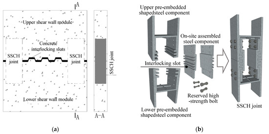
Figure 1.
Design of the prefabricated shear wall with the new SSCH joint: (a) sketch of the prefabricated shear wall with the SSCH joint; (b) details of the SSCH joint.
3. Numerical Model and Validation
3.1. Constitutive Relationship of Concrete and Steel Materials
3.1.1. Constitutive Relationship of Steel Material
The steel adopts ABAQUS’s built-in bilinear dynamic strengthening constitutive model BKIN, which follows the Mises stress yield criterion and strengthening criterion and takes into account the Bauschinger effect of the steel, which can accurately simulate the mechanical performance of the steel under reciprocating loads. The numerical model of steel is Q345, with a yield strength of 345 MPa, an elastic modulus of 2 × 10⁵ MPa, and Poisson’s ratio of 0.3.
3.1.2. Constitutive Relationship of Concrete Material
ABAQUS has three built-in concrete constitutive models: plastic damage constitutive model, smeared cracking model, and brittle cracking model. Among the three constitutive relationship models, the plastic damage constitutive model takes into account the differences in material tensile and compressive properties and reflects them through different damage factors [24], which is used to simulate the stress characteristics of concrete under cyclic or dynamic loads It is easier to converge compared to other models and is not affected by cracks. The plastic damage constitutive model is then adopted in this study.
There are five material parameters for the plastic damage constitutive model that need to be defined firstly: expansion angle, eccentricity, yield strength ratio fb0/fc0, the second stress invariant k in the meridian plane of tension and compression, and the viscosity parameter. The expansion angle and eccentricity define the shape of the flow potential energy surface. The yield strength ratio and the second stress invariant k determine the shape of the yield surface in the plane stress and off plane. The viscosity parameter is closely related to whether the analysis results can converge, and the default value is 0. The larger the viscosity coefficient, the easier the material stiffness and convergence of the analysis. The smaller the viscosity parameter, the closer the calculation results are to the real situation, but the more difficult it is to converge the analysis results [10]. After comprehensive consideration of factors such as analysis accuracy, computational efficiency, and convergence, the final parameter values determined in this study are shown in Table 1.

Table 1.
Parameter values of the concrete plastic damage model.
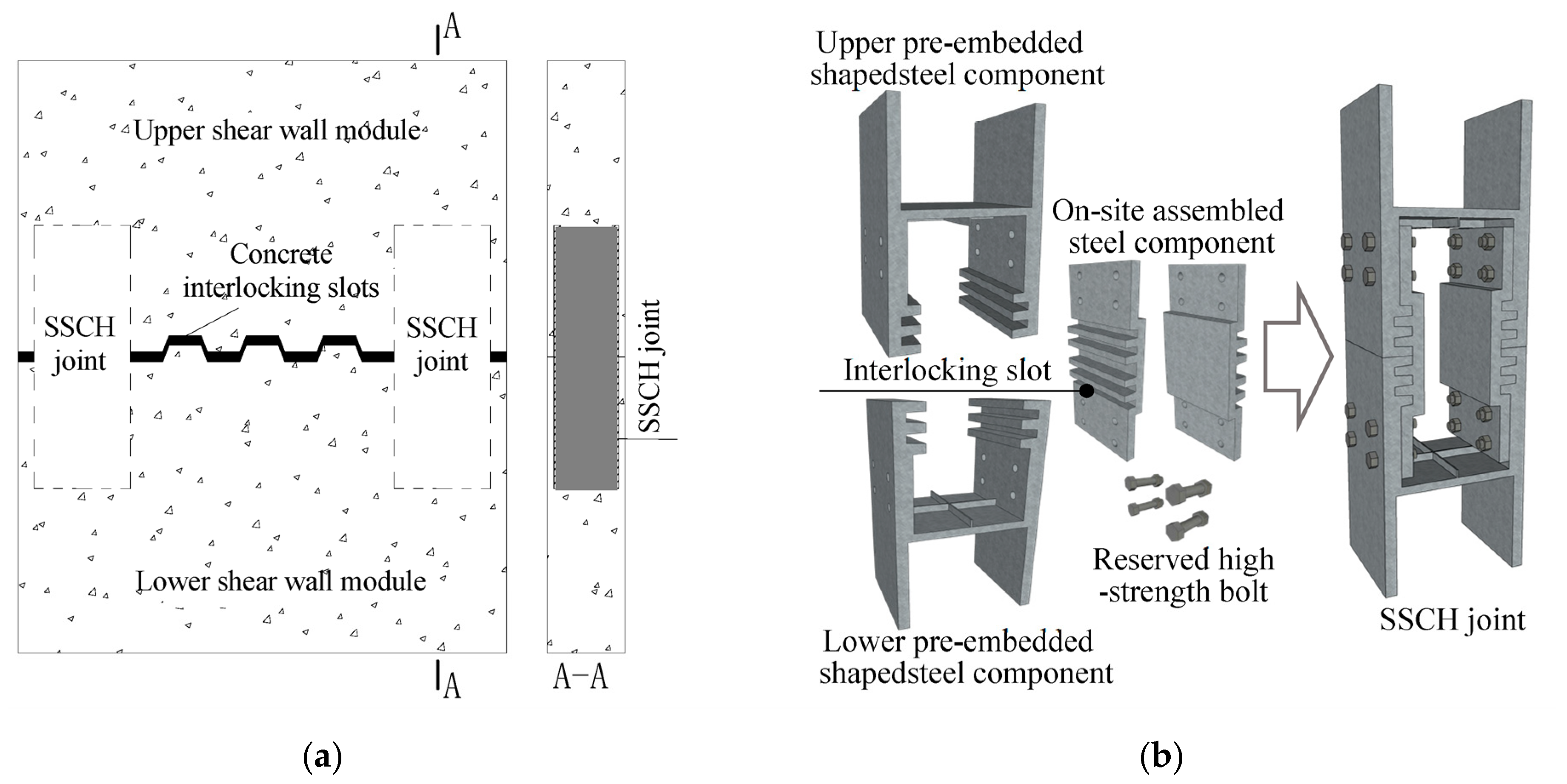
The constitutive definition of concrete consists of two parts: elasticity and plasticity. The elasticity part is determined by the elastic modulus and initial yield strength of concrete. The stress–strain relationship of the plasticity part is relatively complex, which adopts Zhenhai Guo’s model in this study [25]. As shown in Figure 2a, the stress–strain equation can be expressed as follows under uniaxial compression:
where x is the strain, y is the stress, εc is the peak strain, , E0 is an elastic modulus of concrete, fc is concrete axial compressive strength, and αa and αd are parameters determined by fc and , namely, , .
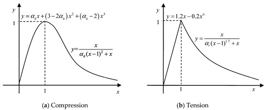
Figure 2.
Stress–strain curves of concrete plastic damage constitutive model.
The stress–strain equation can be expressed as follows under uniaxial tension, as shown in Figure 2b:
where and ft is concrete axial tensile strength.
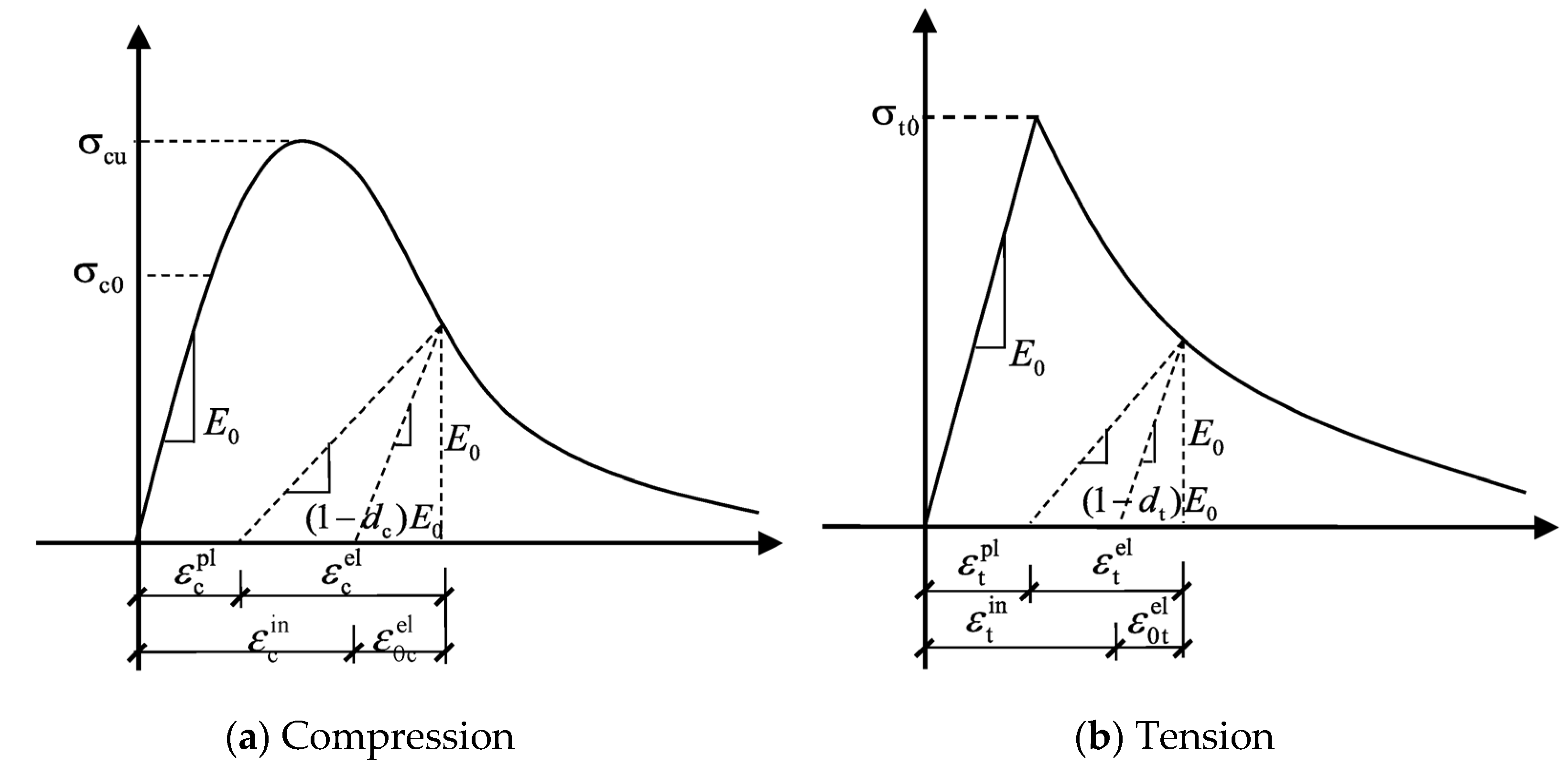
Some phenomena, such as plastic cumulative and stiffness degradation, will be generated for concrete material under tension and compression reciprocating loading, which has great difference with one-way loading. For example, the force–displacement hysteresis curve may be very full, with no pinching phenomenon under reciprocating loading, if the damage factor is not considered, which will then cause over an estimation of energy dissipation capacity of concrete members. Actually, there is a certain pinch phenomenon of hysteresis curves for concrete members in experimental loading [11]. Hence, the concept of damage factor is introduced to describe the complex behavior of concrete under reciprocating loading. Energy equivalence method and graphic method [26] are the commonly used methods employed to calculate the damage factor, and the latter is adopted in this paper, as shown in Figure 3.
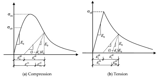
Figure 3.
Stress–strain curve of concrete damage model.
As shown in Figure 3a, the initial relationship between stress and strain is linear when the condition of uniaxial compression. But after the stress arrives to its elastic maximum compressive stress σc0, the relationship will assume the status of a rising curve and then start to decrease in compression when the maximum compressive stress σcu is reached. Finally, unloading begins at stress point σcn. The compressive plastic strain of concrete can be expressed as follows [26]:
Hence, the compressive damage factor can be obtained:
where , is compressive damage factor and . The concrete will be fully damaged when dc = 1, partly damaged when 0 ≤ dc ≤ 1, and not damaged when dc = 0. and are the compressive stress and strain, respectively, of the unloading point. is compressive plastic strain, is compressive nonlinear strain, is compressive linear strain considering damage effect, and is compressive linear strain without damage effect.
The initial relationship between stress and strain is linear when the condition of uniaxial tension. After the stress arrive to its elastic maximum tension stress σt0, the relationship assumes a curve status and then starts to soften in tension. Finally, unloading begins at stress point σtn. The tension plastic strain of concrete can be expressed as follows:
Hence, the tension damage factor can be obtained:
where , is tension damage factor and . The concrete will be fully damaged in tension when dc = 1, partly damaged when 0 ≤ dc ≤ 1, and not damaged when dc = 0. and are tension stress and strain, respectively, of the unloading point. is tension plastic strain, is tension nonlinear strain, is tension linear strain considering damage effect, and is tension linear strain without damage effect. In Equations (4) and (6), the values of bc and bt adopt the suggestion of Birtel and Mark [27], and the two parameters can generally be defined as bc = 0.7 and bt = 0.1. The values of constitutive relationship considering the plastic damage effect of concrete and corresponding damage factors can then be calculated for simulation purpose.
3.2. Validation of a Numerical Model
A numerical model using a computer program ABAQUS 6 software is implemented for the nonlinear dynamic analysis of a reinforced concrete shear wall using finite modeling, material constitutive, and computational procedures described in the previous sections. The numerical model has been studied by Qian et al. [28] using mechanical performance test. Figure 4 shows the specific geometry and rebar details of the shear wall specimen. Table 2 shows the yield strength and ultimate strength of the rebars. The concrete strength grade used in this shear wall is C40, and the axial compression ratio is 0.55. The loading method is first to use force loading, repeat each level of load once, and then use displacement loading with each level of load cycling three times. The maximum loading displacement is 40 mm. The height of the loading point is 2960 mm from the bottom section of the wall. When the bearing capacity of the specimen decreases to 85% of the peak bearing capacity, or when the specimen cannot continue to bear the load, the test stops.
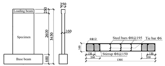
Figure 4.
Specific geometry and rebar details of the shear wall specimen [28].
Table 2.
Yield and ultimate strength of steel.
Based on the sample parameters provided above, the numerical model of the shear wall established in this section is shown in Figure 5, and the model details is shown in Table 3. Solid modeling is adopted in this section. The element type used in concrete is the three-dimensional eight-node reduced integral element C3D8R. The element type used for the reinforcement is the three-dimensional two-node truss element T3D2. The interface between steel bars and concrete adopts a binding relationship. The loading beam, base beam, and the specimen are bound and consolidated together through internal steel mesh and concrete. The boundary condition is defined as bottom consolidation, which constrains the displacement and rotation in three directions. The loading method is consistent with the referenced literature, namely, force loading followed by displacement loading, and with a maximum loading displacement of 40 mm.
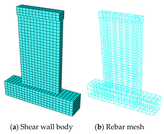
Figure 5.
Numerical model of the shear wall.
Table 3.
Numerical model parameters.
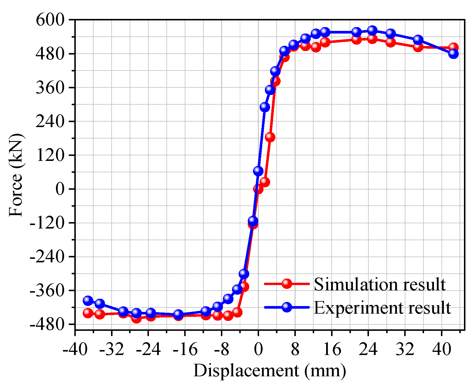
Result comparisons of the load–displacement skeleton curves between the referenced literature and this study are given in Figure 6. It can be found that there is a good fit between the simulation and experiment results. The positive loading forces obtained from experiment and numerical calculation are 561 kN and 532 kN, respectively, with an error of 5.2%. The negative loading forces obtained via experiment and numerical calculation are −445 kN and −458 kN, respectively, with an error of 2.9%. The small difference between the referenced literature and this study may be due to differences in the material models used and in the structure and approximations made in the numerical techniques. Hence, it can be concluded that the numerical model used in this study is reasonable and feasible, which guarantees the reliability of following simulations.

Figure 6.
Load−displacement skeleton curves.
3.3. Model Establishment of the SSCH Joint
ABAQUS software is adopted to build a three-dimensional finite element model of the SSCH joint, as shown in Figure 7. The SSCH joint has dimensions of 200 mm × 240 mm × 680 mm, with the thickness of the steel plate of 20 mm. Q345 is used by the SSCH joint with the yield strength of 345 MPa. The holes in the SSCH joint are filled with C40 concrete. The steel plate and concrete of the SSCH joint are modeled using a three-dimensional solid element C3D8R, which is a linear reduced integral element with eight nodes and six facets. Plastic damage constitutive was adopted by the concrete material. Bilinear dynamic strengthening constitutive was adopted by the steel of the SSCH joint [29]. Finite element mesh generation is a very important step in the entire finite element numerical simulation analysis, and the number of grids directly affects the calculation accuracy and cost. In order to find the most reasonable grid division, comparative model calculations are conducted for 10 different grid divisions, as shown in Table 4.
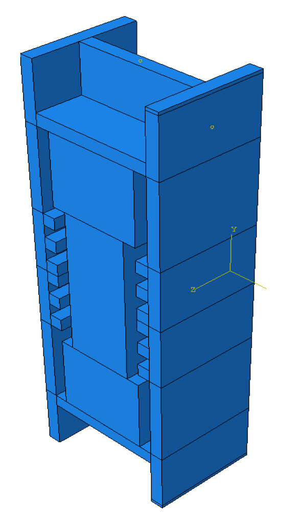
Figure 7.
Numerical model of the SSCH joint.
Table 4.
Model design for different grid divisions.
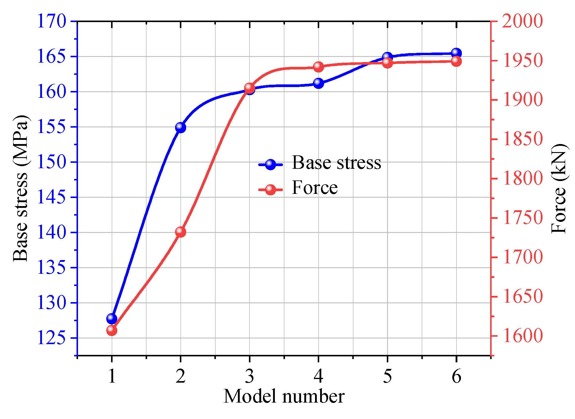
The bottom stress and maximum force of the different models are compared, and the results are shown in Figure 8. It can be found that the stress and maximum load at the bottom of the SSCH joints show a trend of first rapidly increasing, then slowly increasing, and finally tending to remain unchanged. The inflection point of the curve appears in Model 6, where the mesh size of the model is 10 mm. Therefore, the subsequent calculation models all use 10 mm grid size to ensure the rationality of the calculation results.

Figure 8.
Comparison bottom stress and maximum force of the different models.
Another important issue in establishing the SSCH joint model is the contact problem, as there are a large number of contact interfaces, such as the interfaces between the pre-embedded steel components and the on-site assembled steel components, between the steel components and concrete of the SSCH joint. The concrete inside SSCH joint are filled by the micro expansion concrete filled. After the concrete solidifies, it will generate strong pressure on the steel plate groove and increase the friction force between each other. In addition, there are high-strength bolts connecting the steel plate and concrete through it. When the gap between the bolt hole and the bolt is not considered, there is almost no relative displacement between the filled micro expansion concrete and the steel plate. Therefore, the contact interface between steel plate and concrete is defined by binding relationship in simulation [29].
The interfaces between the pre-embedded steel components and the on-site assembled steel components are assembled and transmitted through the interlocking slots. This type of contact interface can transmit pressure to each other under pressure. But when pressure is not present, the contact interface will separate from each other. Obviously, this contact interface cannot be defined as a binding relationship in numerical models. This contact relationship is simulated using a hard contact with friction coefficient in this study. According to the Code for Design of Steel Structures [30], the friction coefficient between the steel interfaces is usually within the range of 0.3–0.5. Therefore, the contact interfaces between the pre-embedded steel components and the on-site assembled steel components is defined as hard contact, with a friction coefficient of 0.5.
4. Parameter Effect of the SSCH Joint
4.1. Calculation Cases
It can be found that the mechanical performance of the SSCH joint is mainly achieved through the buckle connection among the interlocking slots. The design parameters of the interlocking slots will directly affect the transmission of mechanical properties and mechanical behavior of prefabricated shear walls. Therefore, this section will focus on discussing the effect of slot parameters on the mechanical behavior of the SSCH joints, in order to achieve optimal parameter design. The calculation cases are shown in Table 5, which are explained specifically as follows:
Table 5.
Design of the calculation cases.
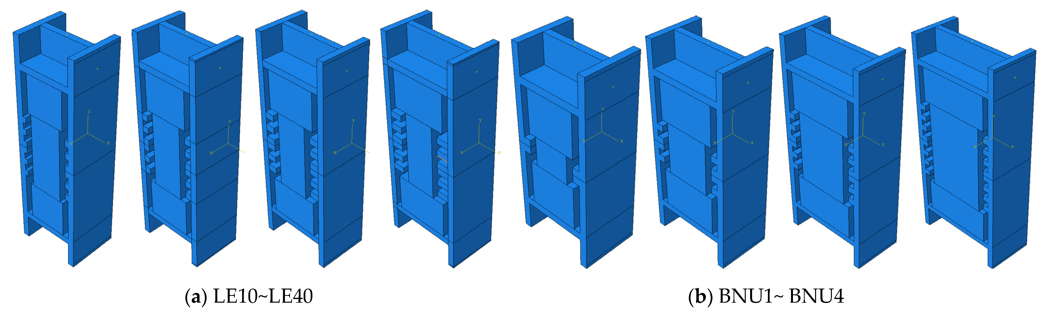
LE10~LE40: Parameter effect of the length of the interlocking slot is discussed on the mechanical behavior of the SSR joint in these four cases, as shown in Figure 9a.

Figure 9.
Schematic diagram of the calculation models.
BNU1~BNU4, CNU1~CNU4: Parameter effect of the number of the interlocking slot is discussed on the mechanical behavior of the SSR joint in these eight cases. As for the cases of BNU1~BNU4, the length of the interlocking slot is defined as 20 mm, as shown in Figure 9b. As for the cases of CNU1~CNU4, the length of the interlocking slot is defined as 30 mm.
TH10~TH40: Parameter effect of the thickness of the interlocking slot is discussed on the mechanical behavior of the SSR joint in these four cases.
ACR3~ACR6: Parameter effect of the axial compression ratio of the interlocking slot is discussed on the mechanical behavior of the SSR joint in these four cases.
4.2. Effect of the Length of the Interlocking Slot
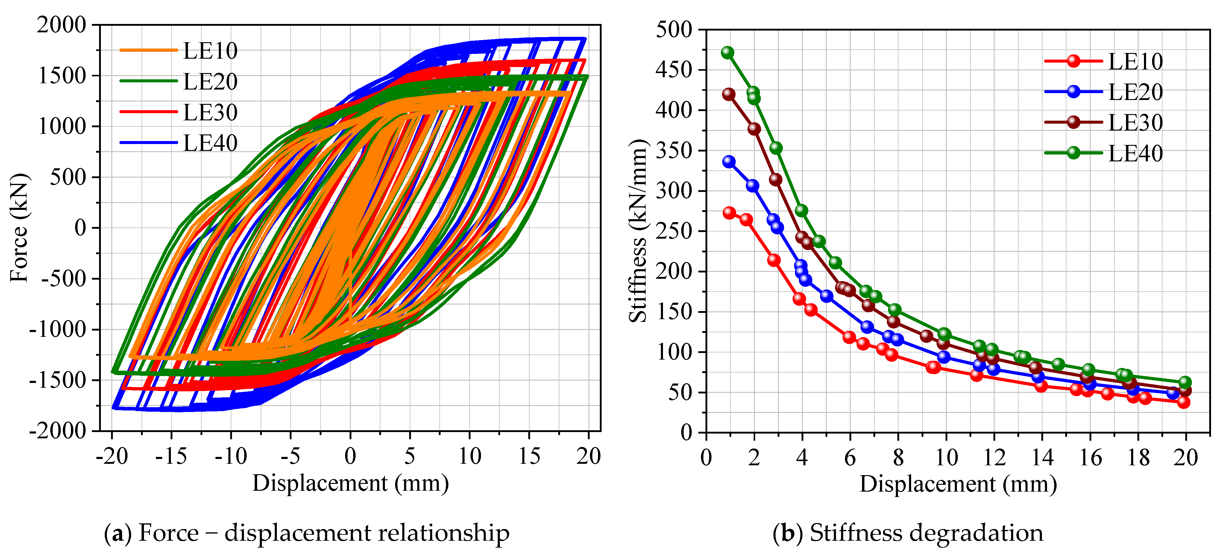
Figure 10 shows a comparison of the force–displacement relationship and the stiffness degradation of the SSCH joints in different lengths of the interlocking slot. Table 6 gives the key mechanical properties of the SSCH joints in different lengths of the interlocking slot. It can be observed that the yield displacement of SSCH joints with different slot lengths is around 6.7 mm, and the ultimate displacement is around 16 mm, without significant difference. However, as the slot length increases, the bearing capacity and the initial stiffness of the SSCH joint gradually increases with the increasing length of the interlocking slot. For example, the yield forces of the cases LE10, LE20, LE30, and LE40 are 1009.4 kN, 1227.8 kN, 1489.6 kN, and 1632.4 kN, respectively. Correspondingly, the peak force are 1243.5 kN, 1428 kN, 1657.5 kN, and 1867.5 kN, respectively. In addition, the energy consumption capacity of the SSCH joints also increases with the increase in slot length. Compared to the SSCH joint with the slot length of 10 mm, the average energy dissipation per cycle of the joint with the slot length of 20 mm increased by 15.27%, and the total energy increased by 16.7%. The average energy dissipation per cycle of the joint with the slot length of 30 mm increased by 16.47%, and the total energy increased by 18.82%. The average energy dissipation per cycle of the joint with the slot length of 40 mm increased by 22.82%, and the total energy increased by 21.78%.

Figure 10.
Curves depicting the force − displacement relationship and stiffness degradation for the cases LE10~LE40.
Table 6.
Key mechanical properties of the SSCH joint in different lengths of the interlocking slot.
The stiffness degradation of the SSCH joints with different slot lengths shows a consistent variation pattern; that is, the decrease is significant in the initial stage of loading, but the decrease trend slows down in the later stage of loading. For the SSCH joint with different slot lengths, although their stiffness gradually increases with the increase in slot length, the amplification in stiffness decreases with the increase in slot length. This phenomenon indicates that an increase in the slot length is beneficial for improving the stiffness of the SSCH joint, but it is only effective within a certain range of slot length. The same phenomenon can also be found in the bearing capacity and energy dissipation of the SSCH joint. Hence, the recommended range for the length of the interlocking slot is 20 mm~30 mm.
Contours of Mises stress with changing of the loading displacement for the Case LE10 and LE30 are shown in Figure 11. It can be found that the Mises stress has an almost consistent development pattern for the Cases. In the initial stage of loading, stress concentration areas appear at the bottom of the steel component and at both ends of the interlocking slot. After that, the stress concentration area slowly expands and begins to spread from the bottom of the steel component to the upper part. In the condition of the same loading displacement, it can be found that the stress diffusion is faster, and the stress concentration range is larger when the length of the interlocking slot is smaller, indicating that increase in the length of the slot is beneficial for improving the bearing capacity of the SSCH joint.
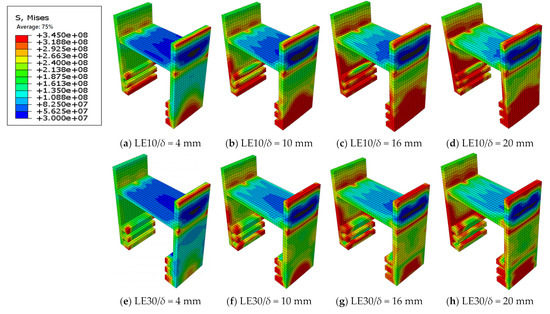
Figure 11.
Contours of Mises stress with changing of the loading displacement for different slot length.
4.3. Effect of the Number of the Interlocking Slot
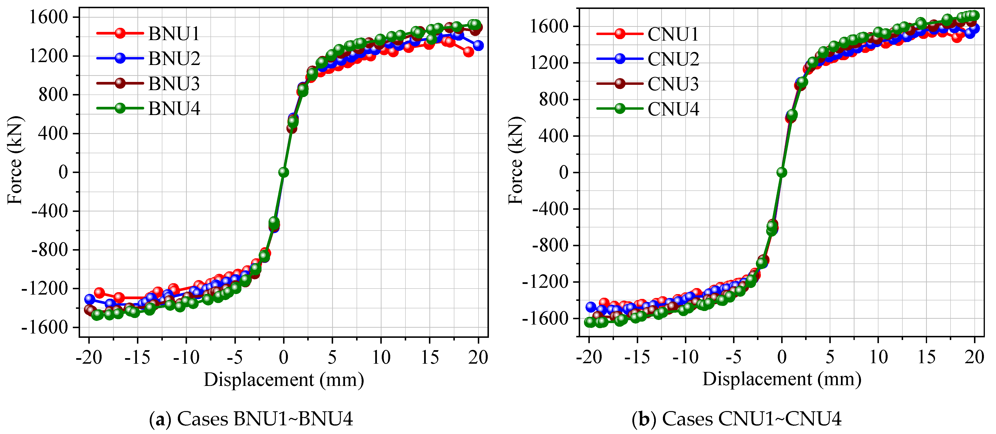
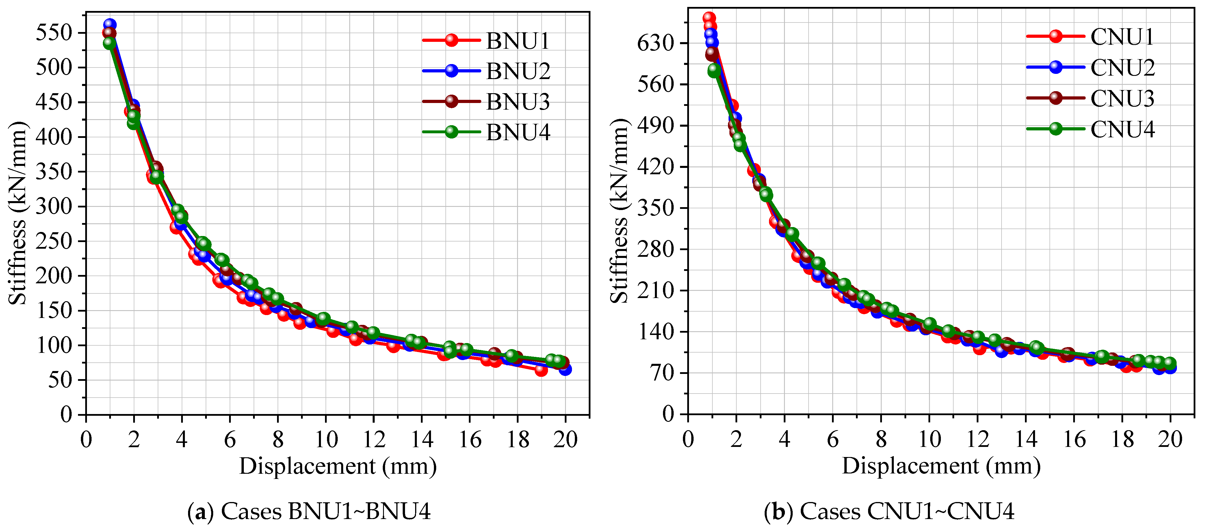
Figure 12 and Figure 13 show the force–displacement relationship and the stiffness degradation of the SSCH joint in different numbers of the interlocking slot. Table 7 gives the key mechanical properties of the SSCH joint in different numbers of the interlocking slot. Under the same length of tooth slots, it can be found that the mechanical behaviors of the SSCH joints, such as load-bearing capacity, stiffness degradation, and ductility, show a consistent trend with the increase in the slot number. For example, the yield and peak forces of the SSCH joint with one interlocking slot and 20 mm slot length are 1026 kN and 1347 kN. Correspondingly, the yield and peak forces with four interlocking slots and 20 mm slot length are 1064.4 kN and 1447.5 kN. The latter only increased by 3.74% and 7.46% compared to the former, respectively. Similarly, when the slot length is 30 mm, the yield and peak forces of the SSCH joints with four interlocking slots only increase by 6.21% and 2.48% compared to joint with one interlocking slot. In addition, under the same condition of the slot length, although the ductility coefficient of the SSCH joints decreases to a certain extent with the increase in the slot number, the degree of decrease is also very small. Under the condition of 20 mm slot length, the ductility coefficient of the SSCH joints with four slots decreases by only 1.86% compared to one slot. Under the condition of 30 mm slot length, the ductility coefficient decreases by 8.48%.
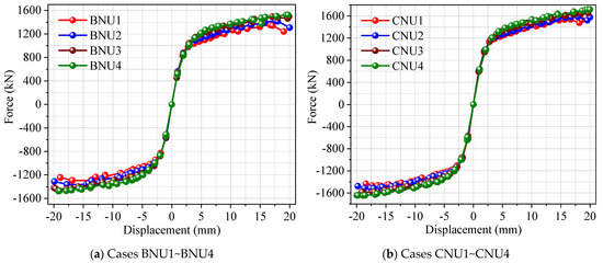
Figure 12.
Force − displacement curves of the SSCH joint in different numbers of the interlocking slot.
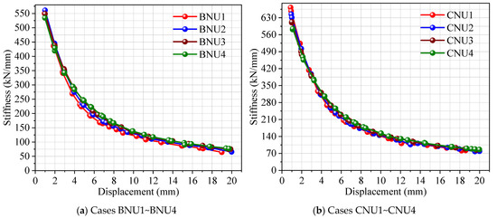
Figure 13.
Stiffness degradation curves of the SSCH joint in different numbers of the interlocking slots.
Table 7.
Key mechanical properties of the SSCH joint in different numbers of the interlocking slots.
Although the mechanical parameters, such as joint bearing capacity, stiffness degradation, and ductility coefficient, do not change significantly with the increase in the slot number, the energy dissipation capacity of the SSCH joints has significantly improved. For example, the total energy dissipation of the cases BNU1, BNU2, BNU3, and BNU4 are 442.48 kN·m, 490.28 kN·m, 552.13 kN·m, and 575.28 kN·m, respectively, and the corresponding growth rates are 10.80%, 24.78%, and 30.01% relative to the joint with one slot. Correspondingly, the total energy dissipation of the cases CNU1, CNU2, CNU3, CNU4 are 479.83 kN·m, 531.92 kN·m, 561.91 kN·m, and 586.97 kN·m, and the corresponding growth rates are 10.86%, 17.11%, and 22.33%. It can be seen that although the energy consumption capacity of the SSCH joints is also increasing with the increase in the slot number, the growth rate is continuously decreasing. As is well-known, the more slots there are, the more complex the processing, transportation, and assembly of the joints. Therefore, considering factors of the complexity of joint construction, the economy of material use, the convenience of on-site assembly, and so on, this study suggests that the number of interlocking slots for the SSCH joint should be two or three.
4.4. Effect of the Thickness of the Interlocking Slot
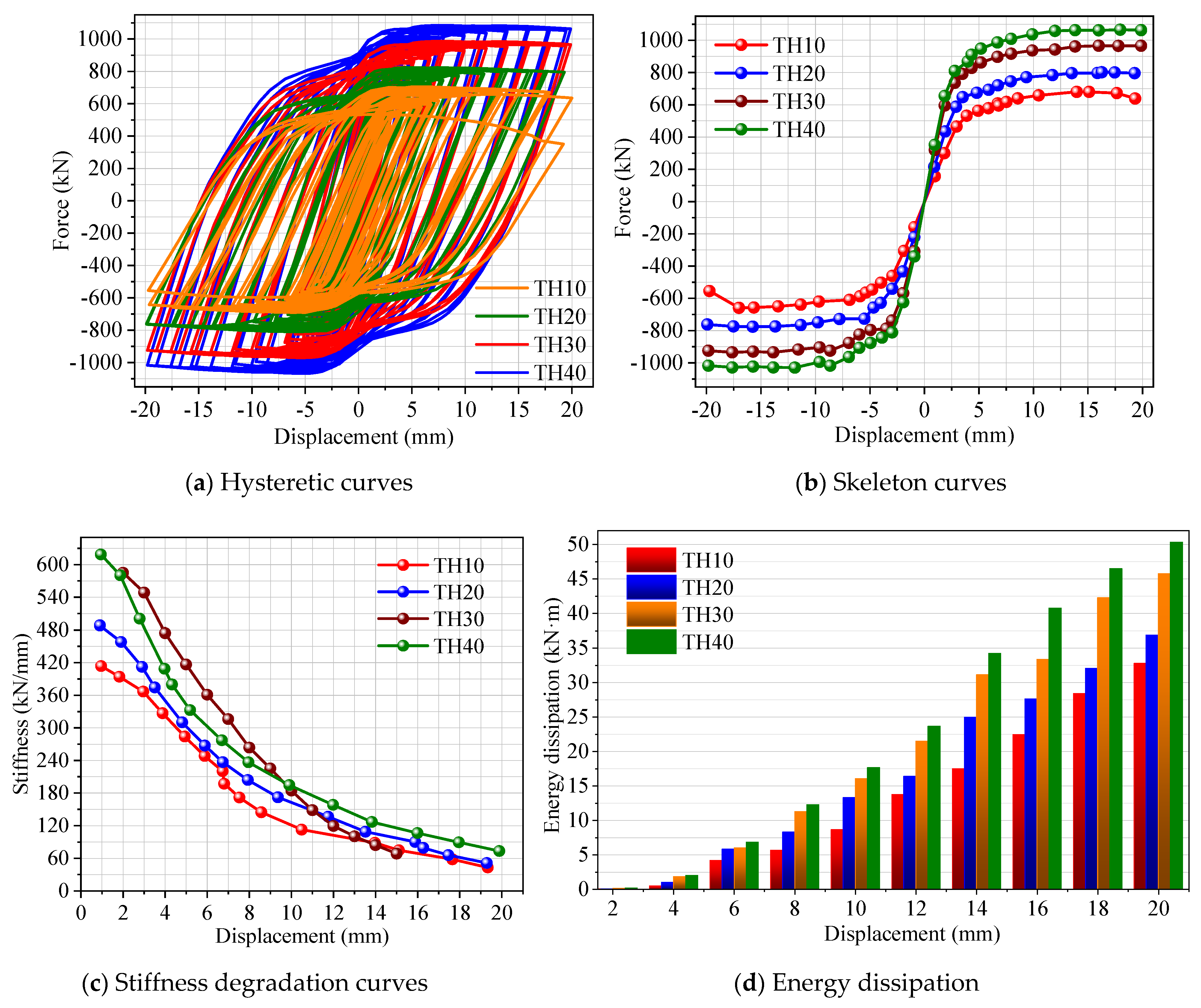
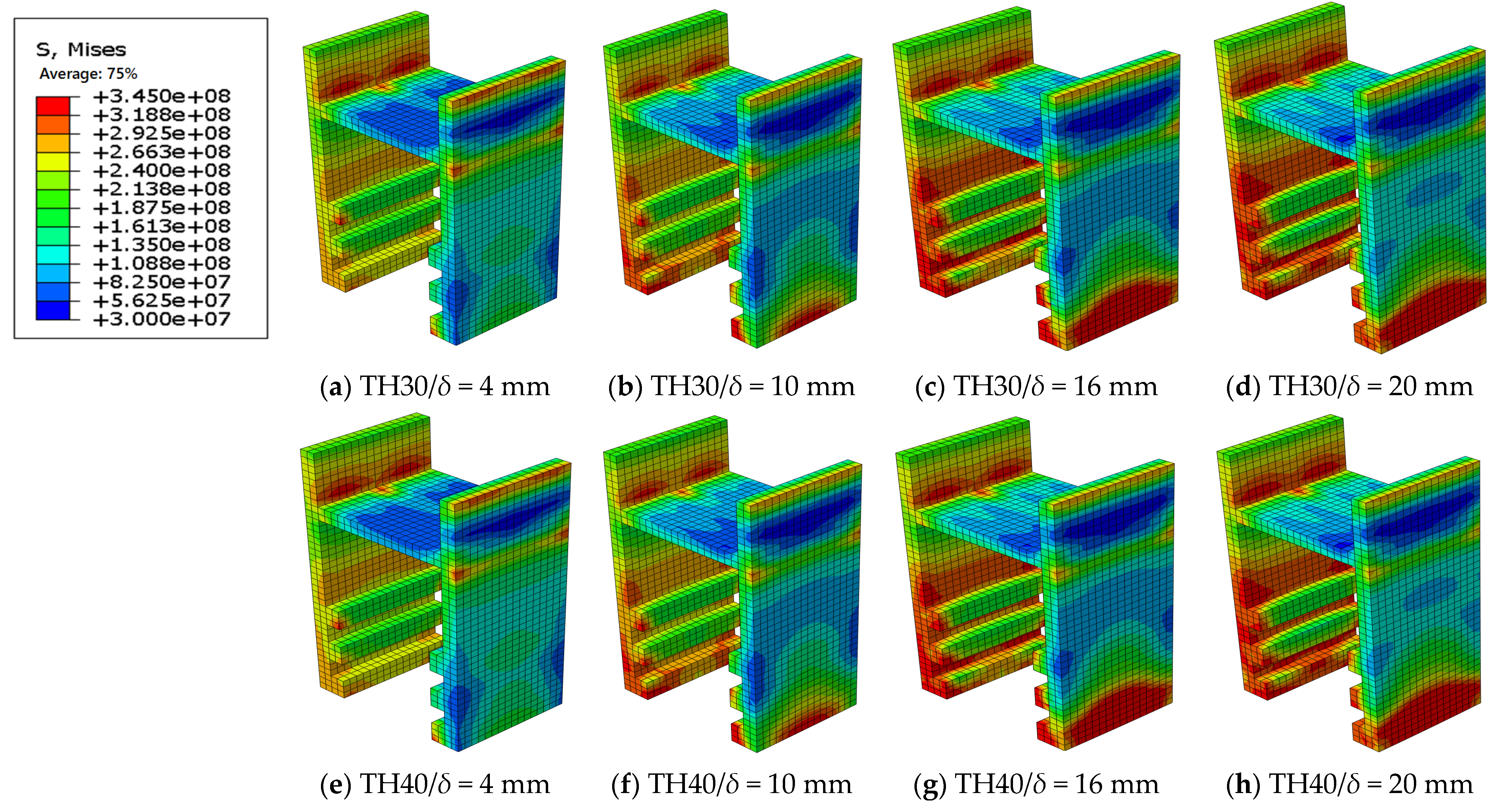
Figure 14 shows the comparisons of hysteretic curves, skeleton curves, stiffness degradation, and energy dissipation of the SSCH joints for the cases TH10~TH40. Table 8 gives the key mechanical properties of the SSCH joint in different thicknesses of the interlocking slot. Contours of Mises stress with changing of the loading displacement for the CaseTH30 and TH40 are shown in Figure 15. It can be observed that the yield displacement, yield force, ultimate displacement, and ultimate force of the SSCH joints all significantly increase with the increase in slot thickness. Compared to the yield force and ultimate force of the SSCH joints with 10 mm slot thickness, the SSCH joints with 20 mm slot thickness are increased by 18.54% and 17.92%, the SSCH joints with 30 mm slot thickness are increased by 47.53% and 42.04%, and the SSCH joints with 40 mm slot thickness are increased by 62.29% and 56.66%, respectively. This indicates that the thickness of the slot steel plate of the SSCH joint is beneficial for significantly improving the load-bearing capacity.

Figure 14.
Mechanical behaviors of the SSCH joints for the cases TH10 ~ TH40.
Table 8.
Key mechanical properties of the SSCH joint in different thickness of the interlocking slot.
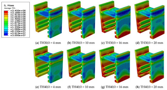
Figure 15.
Contours of Mises stress with changing of the loading displacement for different slot thickness.
It can be observed that there is also a similar trend in the energy consumption capacity of the SSCH joints. Namely, the energy consumption capacity of the SSCH joints gradually increases with the increase in the thickness of the slot steel plate. Compared to the SSCH joint with 10 mm slot thickness, the total energy dissipations of the SSCH joints with a slot thickness of 20 mm, 30 mm, and 40 mm are increased by 35.38%, 57.22%, and 72.94%, respectively. In addition, the stiffness degradation of the SSCH joints also follows a similar pattern. The thicker the slot steel plate, the greater the overall stiffness of the joint, and the slower the degradation effect. Although an increase in the thickness of the slot steel plate will bring superior characteristics, such as bearing capacity, energy consumption, and stiffness degradation, it will also lead to an increase in the joint height and width, which may further cause certain constraints on joint design, cost control, on-site construction, etc. So, the recommended range for the thickness of slot steel plate of the SSCH joint is 20–30 mm. In addition, it can be found that the Mises stress of the SSCH joints gradually increases with increase in loading displacement, and the stress concentration area continuously diffuses from the bottom to the upper part. The stress distribution and diffusion range of the SSCH joint with different slot thicknesses exhibit similar variation patterns.
4.5. Effect of the Axial Compression Ratio
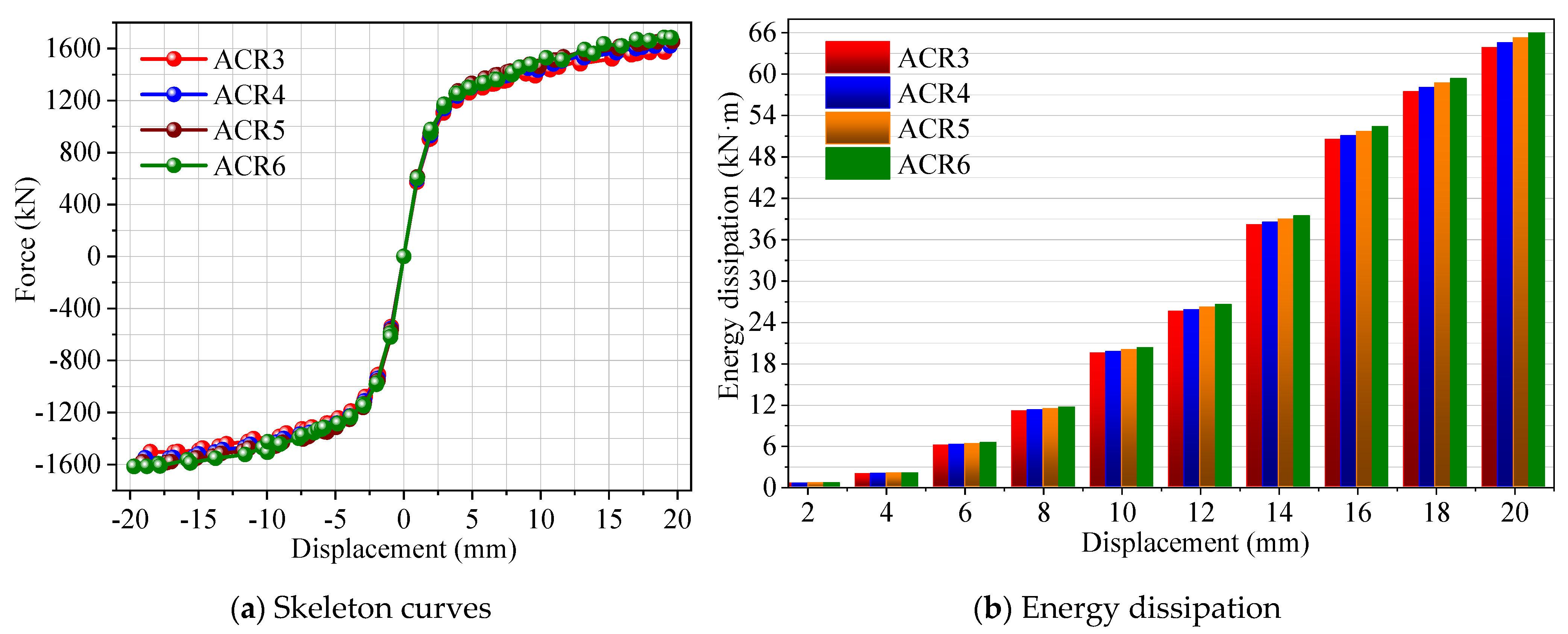
Figure 16 shows the comparisons of the skeleton curves and energy dissipation of the SSCH joints for the cases ACR3~ACR6. Table 9 gives the key mechanical properties of the SSCH joint in different axial compression ratios. It can be observed that the skeleton curves of the SSCH joints under different axial compression ratios exhibit almost identical variation patterns. Under the same loading displacement, the bearing capacity, ductility, and energy dissipation of the SSCH joints also does not differ significantly. For example, the yield force of the cases ACR3~ACR6 are 1039 kN, 1051 kN, 1064 kN, and 1078 kN, respectively, in which the difference between the maximum and minimum values is only 3.75%. Correspondingly, the ductility of the cases ACR3~ACR6 are 4.38, 4.36, 4.41, 4.44, respectively, in which the difference between the maximum and minimum values is only 1.25%. It can then be concluded that the axial compression ratio has a certain effect on the mechanical behaviors of the SSCH joints, but this effect is very small and can be basically ignored.
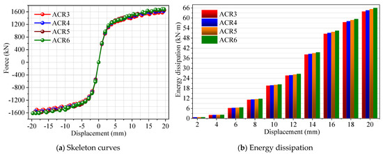
Figure 16.
Mechanical behaviors of the SSCH joints for the cases ACR3 ~ ACR6.
Table 9.
Key mechanical properties of the SSCH joint in different axial compression ratios.
5. Simplified Constitutive Model of the SSCH Joint
5.1. Theory Deduction
According to the deformation characteristics and the degree of transferable bending moment of the connection joints under external forces, joint connections can be divided into rigid connection joints, semi-rigid connection joints, and hinge connection joints. Semi-rigid nodes have greater advantages, which can effectively reflect the bending moment and rotational effects of joints, have simpler construction forms and higher construction efficiency, and also comply with the real situation of common joint connections [31]. The M-θ relationship is also used to characterize the restoring force model of semi-rigid connections, that is, the relationship between the bending moment at the joint connection and the relative rotation angle. Strictly speaking, various types of M-θ relationships are all nonlinear during the entire loading stage, and the diversity of connection forms in practical engineering directly leads to the complexity of the M-θ relationships, which makes it difficult to theoretically derive universally applicable expressions. This section will derive and establish the restoring force constitutive relationship of the SSCH joints based on the bilinear constitutive model based on the M-θ relationship.
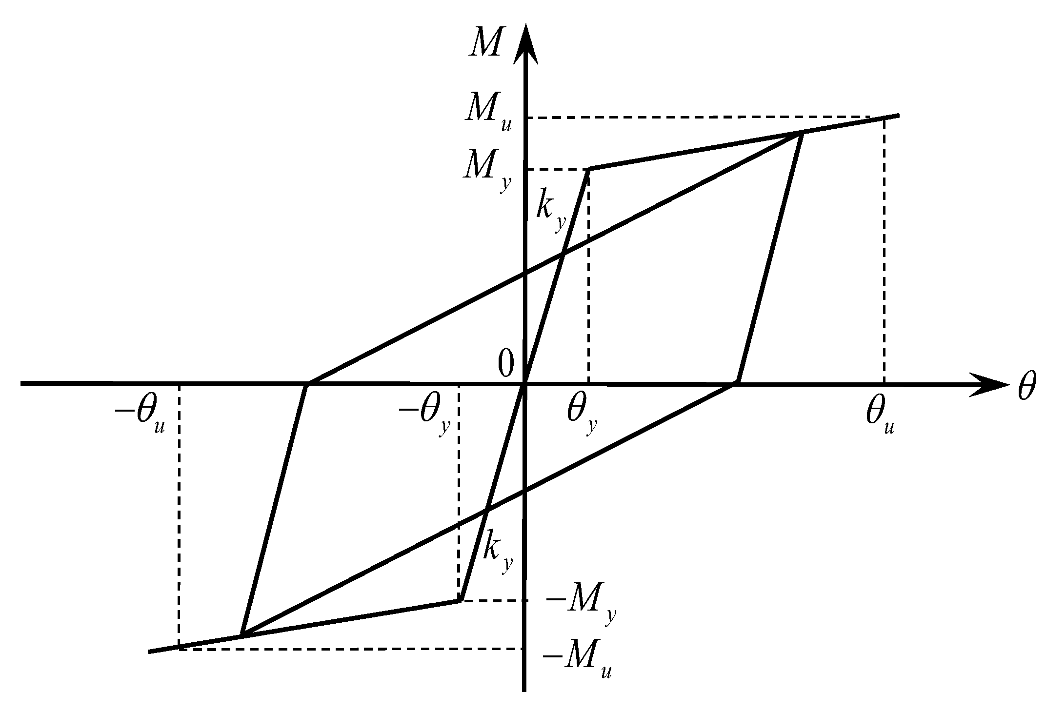
The key to establishing a bilinear M-θ constitutive model lies in the calculation of the parameters are yield and ultimate points, namely, yield and ultimate bending moments and yield and ultimate rotation angles, as shown in Figure 17. Once the four parameters are determined, a bilinear constitutive model can then be established. To obtain the bending moment My at the yield point, it is necessary to first determine the position of the neutral axis of the cross-section. The neutral axis divides the cross-section into two equal areas above the neutral axis, and each element within the cross-section has a compressive stress equaling to the yield stress σy, as shown in Figure 16, in which A1 = A2 = A/2. For rectangular components, the neutral axis is the same for ultimate moment and elastic moment.

Figure 17.
Bilinear constitutive model with the M-θ relationship.
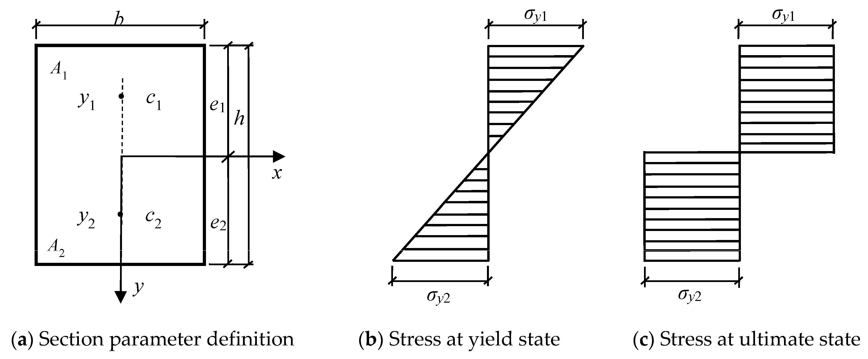
By taking the moment of the force in Figure 18a towards the neutral axis, the ultimate moment Mu of the rectangular cross-section component can be obtained as follows [31]:
where y1 and y2 are the distances from the neutral axis to the centroids c1 and c2 of areas A1 and A2, respectively.

Figure 18.
Stress distribution of rectangular cross-section component.
The ratio of the ultimate moment of a component to its yield moment is called the cross-sectional shape function, usually represented by the shape factor f:
The ultimate modulus Z of rectangular cross-section components is as follows:
As shown in Figure 18a, the distance from the neutral axis to the edge of the elastic core is represented by e. The stress distributions of rectangular cross-section component in the yield state and fully plastic state are shown in Figure 18b and Figure 18c, respectively. The expression for the yield moment can be obtained as follows:
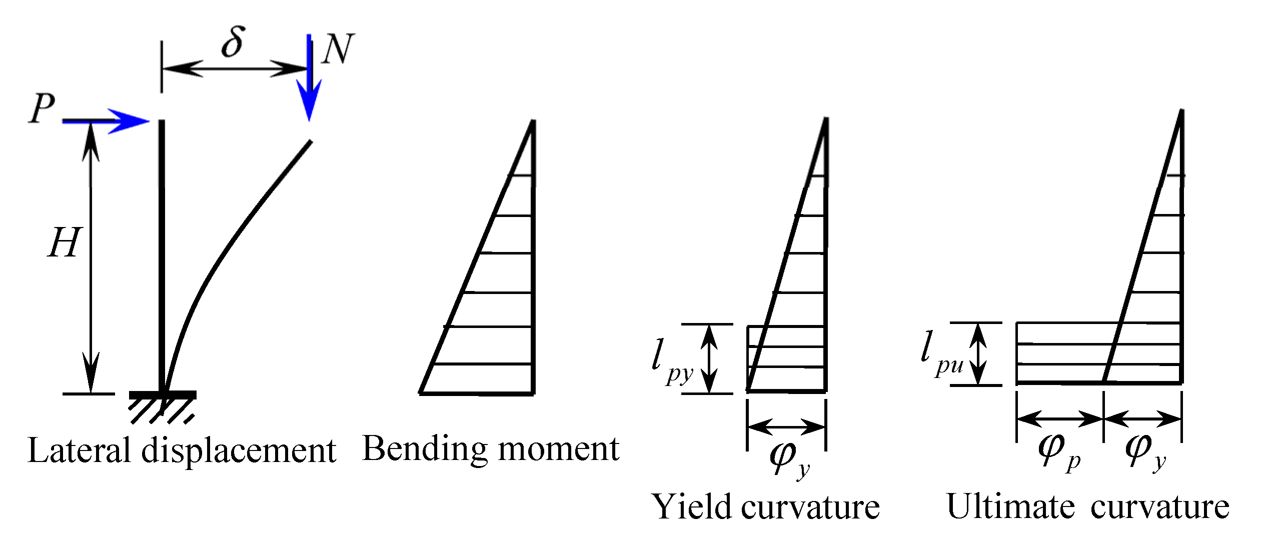
The SSCH joint is modeled as an equivalent cantilever column, and it is assumed that the SSCH joint can mainly be subject to bending failure under the combined action of axial pressure and horizontal force. When using a rod model with plastic hinges at the cantilever column end for nonlinear analysis, the equivalent plastic hinge lengths at the column end in the yield state and ultimate state are lpy and lpu, respectively. If the curvature of the cross-section within this length range is the same and is determined as the yield curvature φy and ultimate curvature φu of the cross-section. The curvature distribution of the SSCH joints at the yield and ultimate stages is shown in Figure 19, in which H is the length from the horizontal force loading point to the column end, and φp is the plastic curvature (φp = φu − φy).
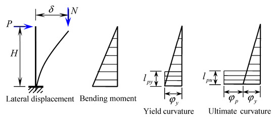
Figure 19.
Lateral displacement and curvature of equivalent cantilever columns for the SSCH joint.
The yield angle θy and ultimate angle θu of the plastic hinge zone can be obtained from Figure 19 according to references [32,33]:
in which, , ,
where εc0 and εcc are the strains of the concrete at the edge of the compression zone of the cross-section when it reaches yield, and ultimately, respectively, εc0 = 0.002, εcc = 0.0033. xny and xnu are depths of the compression zone relative to εc0 and εcc. αy and αu are ratios of the compressive area of concrete to the full cross-sectional area in the yield and ultimate states, fs is steel strength, and deq is the equivalent diameter of the steel in the SSCH joint when it is equivalent to the longitudinal load-bearing steel bar.
Therefore, for the equivalent cantilever column of the SSCH joint, the expressions for the vertex yield displacement and ultimate displacement are as follows [34]:
5.2. Result Discussion
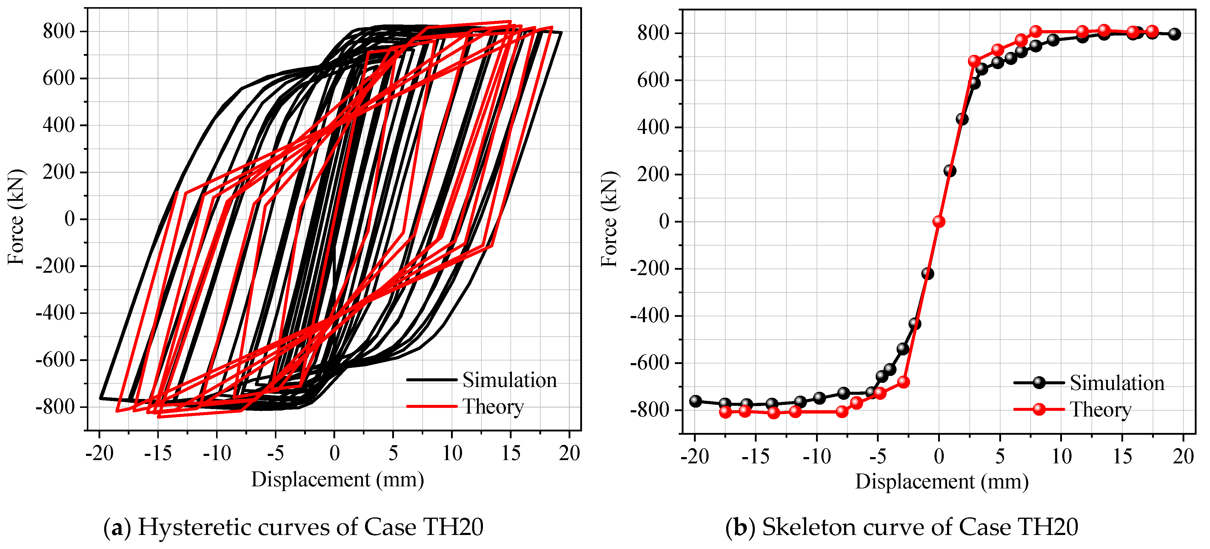
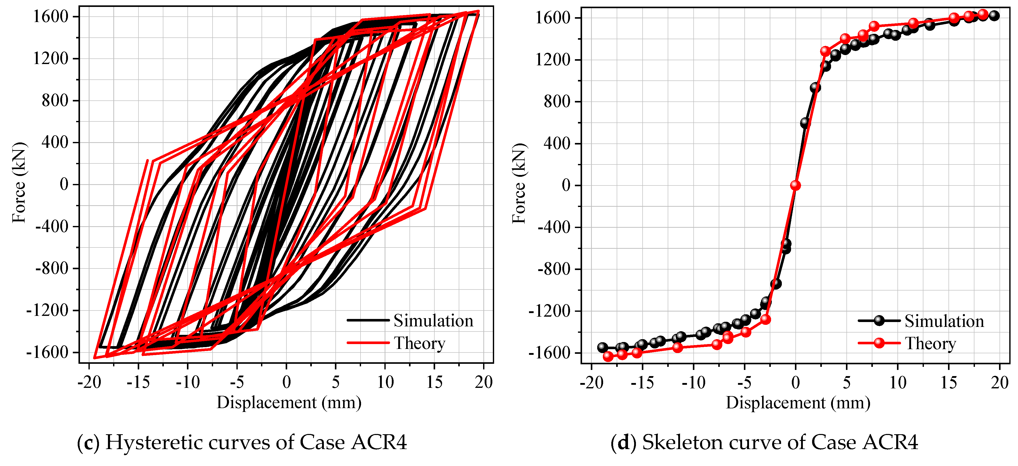
Figure 20 shows the comparisons between the horizontal force–displacement curves calculated based on the simplified constitutive model and the numerical results for some cases above. Table 10 gives the comparative data of the force and displacement at the yield and limit points. It can be found that the hysteretic curves for the simulation and theory have significant differences. The main reason for this is that the proposed M-θ theoretical model adopts the bilinear constitutive law, which causes the inability to capture, effectively, the force–displacement relationship of the SSCH joints in the second and fourth quadrants. However, it can also be found that both the skeleton curves between the simulation result and theory results fit well. The maximum errors for the yield force and the peak force among the six cases given in Table 10 are 7.67% and 4.56%, respectively. The corresponding average error values are 3.11% and 2.67%, respectively. Hence, it can be found that the deduced bilinear constitutive model based on the M-θ relationship can effectively capture the mechanical behavior of the SSCH joints, including stiffness characteristics, yield, and peak mechanical behaviors.
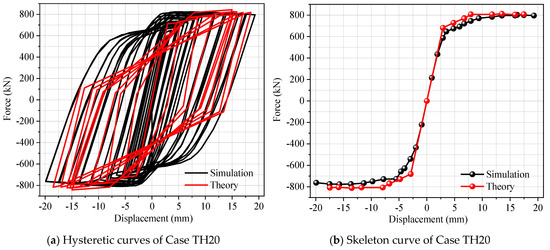
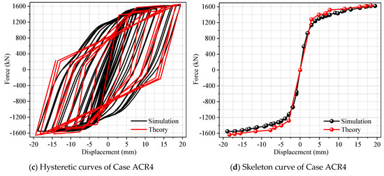
Figure 20.
Comparisons of the hysteresis and skeleton curves for different cases.
Table 10.
Comparative data of parameter indicators at the yield and limit points.
6. Conclusions
A new type SSCH joint used in prefabricated shear wall structure is proposed in this study. Parameter effects of the SSCH joint, such as the length, number, thickness of the interlocking slot, and axial compression ratio, are investigated in detail based on validated numerical model. A simplified constitutive model of the SSCH joint is further deduced. The main results can be summarized as follows:
(1) The force–displacement hysteresis curve of the SSCH joint is relatively full and no pinching phenomenon is found. The ductility coefficients of the SSCH joint are all beyond 4 for the investigated 20 Cases. It can be concluded that the proposed SSCH joint can provide stable shear capacity and superior energy dissipation capacity, which can serve as a reliable shear connection key for the assembly of prefabricated shear wall structures.
(2) The length and thickness of the interlocking slot have a great impact on the mechanical behavior of the SSCH joint, especially for the slot thickness. Compared to the SSCH joint with 10 mm thickness, the ultimate force and energy dissipation of the SSCH joint with 40 mm thickness are increased by 62.29% and 72.94%, respectively. On the contrary, the slot number and axial compression ratio have less effect on mechanical properties and can be ignored. To guarantee more superior mechanical behaviors, it is suggested to design the SSCH joint with a slot length of 20~30 mm, a slot number of two or three, and a slot thickness of 20~30 mm.
(3) The bilinear constitutive model based on the M-θ relationship is advanced, in which the moment and rotation angle calculation formulae for two control points, namely, the yield and limit points, on the skeleton line of the restoring force model are deduced. Based on comparison with numerical results, it can be found that the advanced simplified model can effectively capture the mechanical characteristics of the SSCH joints.
Author Contributions
Conceptualization, Data curation, Funding acquisition, X.W.; Investigation, Project administration, Resources, Y.W.; Conceptualization, Visualization, Writing—review & editing, S.J.; Formal analysis, Methodology, Software, Validation, Writing—original draft, M.L.; Conceptualization, Methodology, Supervision, Writing—original draft, Writing—review & editing, D.W. All authors have read and agreed to the published version of the manuscript.
Funding
This project is supported by the National Natural Science Foundation of China (52378496, 52178467), Technology Project of China Southern Power Grid (037700KK52220039) and the Science and Technology Project of Guangzhou City (202235058).
Data Availability Statement
The data presented in this study are available in article.
Acknowledgments
All statements, results, and conclusions are those of the researchers and do not necessarily reflect the views of these foundations. The authors also sincerely thank the anonymous reviewers for their insightful comments and suggestions.
Conflicts of Interest
Authors X.W., Y.W. and S.J. were employed by the company Power Grid Planning Research Center of Guangdong Power Grid Co., Ltd. The remaining authors declare that the research was conducted in the absence of any commercial or financial relationships that could be construed as a potential conflict of interest.
References
- Singhal, S.; Chourasia, A.; Chellappa, S.; Parashar, J. Precast reinforced concrete shear walls: State of the art review. Struct. Concr. 2019, 20, 886–898. [Google Scholar] [CrossRef]
- Hemamalini, S.; Vidjeapriya, R.; Jaya, K.P. Performance of precast shear wall connections under monotonic and cyclic loading: A state-of-the-art review. Iran. J. Sci. Technol.-Trans. Civ. Eng. 2021, 45, 1307–1328. [Google Scholar] [CrossRef]
- Men, J.J.; Shi, Q.X.; He, Z.J. Optimal design of tall residential building with RC shear wall and with rectangular layout. Int. J. High-Rise Build. 2014, 3, 285–296. [Google Scholar]
- Chu, M.; Liu, J.; Sun, Z. Experimental study on mechanical behaviors of new shear walls built with precast concrete hollow moulds. Eur. J. Environ. Civ. Eng. 2019, 23, 1424–1443. [Google Scholar] [CrossRef]
- Ali, M.M.; Osman, S.A.; Husam, O.A. Numerical study of the cyclic behavior of steel plate shear wall systems (SPSWs) with differently shaped openings. Steel Compos. Struct. 2018, 26, 361–373. [Google Scholar]
- Mao, H.; Qin, G.C.; Lan, T. Study on the seismic performance of box-plate steel structure modular unit. Adv. Mater. Sci. Eng. 2019, 4, 4561631. [Google Scholar] [CrossRef]
- Nguyen, N.H.; Whittaker, A.S. Numerical modelling of steel-plate concrete composite shear walls. Eng. Struct. 2017, 150, 1–11. [Google Scholar] [CrossRef]
- Chu, M.; Wang, B.; Liu, J.; Zhang, P.; Li, X.; An, N. Experimental study on mechanical behavior of precast concrete shear walls with mortise-tenon joints. J. Build. Struct. 2021, 42, 173–182. [Google Scholar]
- Nie, J.-G.; Hu, H.-S.; Fan, J.-S.; Tao, M.-X.; Li, S.-Y.; Liu, F.-J. Experimental study on seismic behavior of high-strength concrete filled double-steel-plate composite walls. J. Constr. Steel Res. 2013, 88, 206–219. [Google Scholar] [CrossRef]
- Wang, D.Y.; Xu, S.C.; Yang, Y.; Mao, J.H.; Zhu, Y.; Guo, D.W.; Nie, Z.L. Study on seismic behaviors of steel–concrete composite shear walls with novel corner designs. J. Build. Eng. 2023, 70, 106339. [Google Scholar] [CrossRef]
- Han, Q.H.; Wang, D.Y.; Zhang, Y.S.; Tao, W.J. Experimental investigation and simplified stiffness degradation model of precast concrete shear wall with steel connectors. Eng. Struct. 2020, 220, 110943. [Google Scholar] [CrossRef]
- Soudki, K.A.; West, J.S.; Rizkalla, S.H.; Blackett, B. Horizontal connections for precast concrete shear wall panels under cyclic shear loading. PCI J. 1996, 41, 64–80. [Google Scholar] [CrossRef]
- Zhao, B.; Wang, Q.; Lu, X. Research on seismic behavior of precast concrete walls with fully assembled horizontal joints. J. Build. Struct. 2018, 39, 48–55. [Google Scholar]
- Cheng, B.; Cai, Y.; Looi, D.T.W. Experiment and numerical study of a new bolted steel plate horizontal joints for precast concrete shear wall structures. Structures 2021, 32, 760–777. [Google Scholar] [CrossRef]
- Wei, H.; Li, Q. Experimental study on seismic behavior of prefabricated RC shear walls with horizontal joints welded by steel plates. J. Build. Struct. 2020, 41, 77–87. [Google Scholar]
- Perez, F.J.; Pessiki, S.; Sause, R. Lateral load behavior of unbonded post-tensioned precast concrete walls with vertical joints. PCI J. 2004, 49, 48–64. [Google Scholar] [CrossRef]
- Chu, M.; Xiong, C.; Liu, J.; Sun, Z. Experimental study on shear behavior of two-way hollow core precast panel shear wall with vertical connection. Struct. Des. Tall Spec. Build. 2021, 30, e1814. [Google Scholar] [CrossRef]
- Huang, W.; Miao, X.W.; Zhao, Y.Y.; Yu, G.; Zhang, J.R.; Fan, Z.H. Experimental study on seismic performance of fully assembled composite walls with vertical joints using different dry connections. J. Build. Struct. 2020, 41 (Suppl. 2), 114–122. [Google Scholar]
- Li, H.; Chen, W.; Huang, Z.; Hao, H.; Ngo, T.T.; Pham, T.M.; Yeoh, K.J. Dynamic response of monolithic and precast concrete joint with wet connections under impact loads. Eng. Struct. 2020, 250, 113434. [Google Scholar] [CrossRef]
- Zhu, G.; Ma, Y.X.; Tan, K.H. Experimental and analytical investigation on precast concrete-encased concrete-filled steel tube column-to-column dry connections under axial tension. Structures 2022, 45, 523–541. [Google Scholar] [CrossRef]
- Li, W.; Gao, H.; Xiang, R.; Du, Y. Experimental study of seismic performance of precast shear wall with a new bolt-plate connection joint. Structures 2021, 34, 3818–3833. [Google Scholar] [CrossRef]
- Fu, Y.; Fan, G.; Tao, L.; Yang, Y.; Wang, J. Seismic behavior of prefabricated steel reinforced concrete shear walls with new type connection mode. Structures 2022, 37, 483–503. [Google Scholar] [CrossRef]
- Xue, W.C.; Li, Y.; Cai, L.; Hu, X. Seismic Performance of Precast Concrete Composite Shear Walls with Multiple Boundary Elements. J. Earthq. Tsunami 2019, 13, 1940006. [Google Scholar] [CrossRef]
- Fintel, M. Performance of buildings with shear walls in earthquakes of the last thirty years. PCI J. 1995, 40, 62–80. [Google Scholar] [CrossRef]
- Guo, Z.H. Principles of Reinforced Concrete Structure; Science Press: Beijing, China, 1998. [Google Scholar]
- Qian, J.R.; Zhao, Z.Z.; Duan, A.; Xia, Z.F.; Wang, M.D. Pesudo-dynamic tests of a 1:10 model of pre-stressed concrete containment vessel for CNP 1000 nuclear power plant. China Civ. Eng. J. 2007, 40, 7–13. [Google Scholar]
- Birtel, V.; Mark, P. Parameterised finite element modelling of RC beam shear failure. In Proceedings of the 19th Annual International ABAQUS Users’ Conference, Boston, MA, USA, 23–25 May 2006; pp. 95–108. [Google Scholar]
- Qian, J.R.; Zao, J.; Ji, X.D. Experimental study on seismic behavior of steel tube-reinforced concrete composite shear walls with high axial compressive load ratio. J. Build. Struct. 2010, 31, 5–13. [Google Scholar]
- Gao, L.B.; Chen, Q.G. An anisotropic damage constitutive model for concrete and its applications. Appl. Mech. 1988, 65, 578–583. [Google Scholar]
- GB 50017-2017; Standard for Design of Steel Structures. China Architecture and Building Press: Beijing, China, 2017.
- Wang, X.W.; Sun, L. Research on the performance of steel frame semi rigid connections. J. Wuhan Univ. Technol. 2002, 21, 65–72. [Google Scholar]
- Qian, J.R.; Liu, X.M. Test of seismic behavior of FRP-concrete-steel double-skin tubular columns. China Civ. Eng. J. 2008, 41, 29–36. [Google Scholar]
- Seible, F.; Priestley, M.J.N.; Hegemier, G.A. Seismic retrofit of RC columns with continuous carbon fiber jackets. J. Compos. Constr. 1997, 1, 52–62. [Google Scholar] [CrossRef]
- Qian, J.R.; Liu, X.M. A hysteretic model of moment-rotation relationship for plastic hinge zone of FRP-concrete-steel double shin tubular columns. Eng. Mech. 2008, 25, 48–52. [Google Scholar]


Disclaimer/Publisher’s Note: The statements, opinions and data contained in all publications are solely those of the individual author(s) and contributor(s) and not of MDPI and/or the editor(s). MDPI and/or the editor(s) disclaim responsibility for any injury to people or property resulting from any ideas, methods, instructions or products referred to in the content. |
© 2023 by the authors. Licensee MDPI, Basel, Switzerland. This article is an open access article distributed under the terms and conditions of the Creative Commons Attribution (CC BY) license (https://creativecommons.org/licenses/by/4.0/).