Abstract
Enclosed airspaces of various effective emittances exist in the building envelope in walls, roofs, and double/triple glazing windows, curtain walls and skylight devices. Assessing the energy performance of a building component with enclosed reflective airspaces requires evaluation of all modes of heat transport inside the airspace. The thermal resistance (R-value) of the enclosed airspaces depends on the dimensions and orientation of the airspace, and the emittance and temperature of all surfaces that bound the airspace. To the best of our knowledge, the existing methods used around the world to evaluate the airspace thermal performance (e.g., ISO 6946, AUS/NZ 4859, and methods based on the U.S. NBS data) are one-dimensional and assume isothermal conditions on the hot and cold surfaces. In actual applications, however, the temperatures of both the hot and cold surfaces vary (i.e., they are non-isothermal), and the heat transfer takes place via conduction, convection and surface-to-surface radiation. In some cases, convection is absent or negligible, as is the case for downward heat flow or situations with a small temperature difference between the hot and cold surfaces. Radiation transport is significantly reduced by the presence of a low-emittance surface in the heat flow path. One of the goals of this study is to answer the question “is it a good assumption to use the isothermal conditions on both the hot and cold surfaces for determining/reporting the R-value of enclosed airspaces for different building applications?” A complete evaluation of the thermal performance of enclosed airspaces that includes the impact of bounding materials can now be undertaken in multiple dimensions with convective transport described by computational fluid dynamics. In addition to providing a relatively complete evaluation of the thermal performance of the enclosed airspaces, the adequacy of popular simplifying assumptions can be evaluated. This paper describes the computational process used, along with examples of the variation in thermal resistance with the airspace aspect ratio, realistic thermal boundary conditions and radiative heat transport on all surfaces that bound the airspace. The analysis completed in this research shows that the assumption of isothermal hot and cold surfaces affects calculated R-values for enclosed reflected airspaces by less than 3%. This was demonstrated for the five conventionally considered heat-flow directions and effective emittances from 0 to 0.82.
1. Introduction
Reflective Insulations (RIs) and related reflective products are applied in buildings and equipment to reduce heat loss in cold climates or heat gain in hot climates. There is a vast body of literature dealing with the use of reflective insulation in buildings. Pratt’s monograph “Heat Transmission in Buildings” contains a chapter that summarizes the understanding of the thermal resistance of enclosed airspaces in buildings [1]. A text book by Wilkes [2] contains a chapter on reflective insulation that contains experimental work and provides guidance for the use of reflective insulations. Detailed information about reflective insulation assemblies was published in the U.K. by Nash et al. [3]. The U.K. publication included design data and installation instructions. Hollingsworth published thermal test results for three multi-layer reflective insulation assemblies and compared the results with calculations using methods accepted at that time [4]. Hollingsworth concluded that the calculated R-values overstated the observed performance. The published research on reflective insulation was reviewed by Lee et al. [5], and another review was published by Tenpierik and Hasselaar [6]. Research completed at the Florida Solar Energy Center on reflective materials used in residential attics was reported by Fairey [7] and the term “radiant barrier” was introduced. Field data on reflective insulation used in the cold climate of Alaska was contained in a report by Craven and Garber-Slaght to document cold weather performance [8].
Research related to reflective systems appeared in the literature as early as 1878 [9], while utilization of the technology was enhanced in 1955 with the publication of Housing Research Paper 32 (HRP 32) that contained the results of a major reflective insulation test program carried out at the U.S. National Bureau of Standards (NBS) [10,11]. The NBS data were obtained for a single airspace aspect ratio, with a few exceptions in the 1991 data from Tye and Desjarlais [12]. Reflective insulation products have at least one surface of low emittance facing an airspace [13]. Regarding reflective insulations use in buildings, enclosed airspaces of various effective emittances exist in building envelope components such as walls, roofs, and double/triple pane windows, curtain walls and skylight devices. Assessing the energy performance of a building assembly with reflective insulation products requires knowledge of the thermal resistance (R-value) of the enclosed airspaces. Note that reflective insulation assembly contains enclosed airspace in which the term “enclosed” is critical. This is because the main difference between reflective insulation and radiant barrier is the airspace condition, in which the radiant barrier system is defined as a system that consists of a low-emittance surface bounded by an “open” airspace. Vrachopoulos et al. [14] provided observations on the overall building energy efficiency achieved with reflective insulation, while Escudero et al. [15] published similar type data for radiant barrier assemblies. Medina [16] developed a computational model for the performance of attic radiant barriers and showed the dependence of savings due to radiant barrier installations decline as the amount of conventional insulation present in the attic increased. Data for the performance of attic radiant barriers in tropical regions published by Miranville et al. [17] provide support for the use of this technology in hot–humid climates.
Recently published research on reflective technology includes field data for reflective insulation used in southern Europe [18]. The stated objective of this research was to determine the benefit of reflective insulation in comparison with other insulating materials. Research in the Gulf Coast region of the United States showed that a reflective product installed in residential attics saved 8 to 25% of the energy load [19]. A computational evaluation of reflective insulation performance in the Czech Republic was reported by Ficker in 2022 [20], while a field evaluation by Teh et al. [21] addressed performance in a Southeast Asian environment. Lee et al. [5] provided an extensive review of radiant barrier and reflective insulation research compiled during 2016. The use of reflective insulation in many areas of the world has been evaluated in recent years.
The R-value of enclosed airspaces depends on the dimensions and orientation of the airspace, the heat-flow direction through the airspace and the values of the emittance and temperature of all surfaces that bound the airspace. To the best of our knowledge, all existing calculation methods used around the world (e.g., IEA [22], ISO 6946 [23], methods based on U.S. NBS data [10,11] that were used in various editions of the ASHRAE Handbook of Fundamentals [24,25,26], Reflective Airspace Tool [27] as well as all available correlations in the literature [28] use the assumption of isothermal conditions for both the hot surface and cold surface to determine and report R-values of enclosed airspaces. Furthermore, the measured R-values for enclosed airspaces from the tests using, for example, the guarded hotbox in accordance with the standard test method ASTM C1224 [29] or heat flow meter apparatus in accordance with the standard test method ASTM C518 [30] are reported at isothermal conditions for the hot surface and the cold surface, despite the fact that the temperatures of these surfaces are not uniform, as will be shown later in more detail in this study. In these tests, however, the isothermal conditions of both hot and cold surfaces of the enclosed airspaces are obtained from the area-weighted average temperatures of the metering areas (e.g., see the ASTM C1224 [29] and ASTM C518 [30] for more details). The R-value of the enclosed airspace obtained with the isothermal assumption for both the airspace hot and cold surfaces is used to determine the effective R-value. In the actual applications, however, both the airspace hot surface temperature and cold surface temperature are not uniform (i.e., non-isothermal). For given airspace dimensions, this study will show that the shapes of the temperature distributions on the hot and cold surfaces of the airspace are greatly non-uniform and depend on the orientation, effective emittance, heat-flow direction and operating conditions. Consequently, one question to be answered in this study is “is it a good assumption to use the isothermal conditions for both the hot surface and the cold surface for determining and/or reporting the R-values of enclosed airspaces for different building applications for subsequent use these R-values in energy simulation models to assess the overall building performance?”
The measurement of the thermal resistance of enclosed reflective airspaces using a hotbox facility generally provides a result based on heat flow across a fixed region: the metering area [31]. The resulting R-value is associated with the distance between the hot and cold surfaces of the test specimen. Since, in this case, a heat transfer involves radiation (and often natural convection), it is reasonable to expect that the thermal resistance will depend on the airspace dimensions in addition to the thickness. This research includes evaluation of airspace thermal resistance as a function of the aspect ratio (length divided by thickness). This allows a more detailed determination of airspace thermal resistances than the use of a single dimension such as thickness [28].
2. Objectives
As the existing methods (e.g., ISO 6946 [23] and ASHRAE [24,25,26]) for determining the R-values of enclosed airspaces are based on radiative heat transport between two large/infinite parallel surfaces [32], the heat transfer by radiation at the two ends, parallel to the heat-flow direction, of the enclosed airspace, with emittance of E3 (see Figure 1), is not included. One of the objectives of this study is to investigate the effect of the heat transfer by radiation at the two ends of the enclosed airspace on the R-value. As indicated earlier, the effect of airspace aspect ratio (AR = Length (H)/Thickness (D)) is not accounted for in the existing methods [24,25,26]. Quantitative results are provided in this paper regarding the effect of the airspace aspect ratio on its R-value.
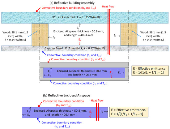
Figure 1.
Schematics for: (a) reflective building assembly and (b) reflective enclosed airspace with convective boundary conditions.
Most of the thermal resistances (R-values) of enclosed airspaces (if not all, to the best our knowledge) that are available in the literature and handbooks are given in terms of uniform hot surface temperature, TH; and uniform cold surface temperature, TC (i.e., isothermal conditions on both the hot and cold surfaces). In this study, the corresponding enclosed airspace thermal resistance is called “R-value based on isothermal conditions, R2a and R2b”. These R-values are currently being used to assess the energy performance of building components incorporating enclosed airspaces (walls and roofs, and multi-pane glazing systems such as windows, curtain walls and skylights). On the other hand, due to the three modes of heat transfer inside the airspace, the actual temperature distributions on the hot surface and the cold surface of enclosed airspaces are not uniform. The corresponding enclosed airspace thermal resistance in this case is called “R-value based on convective conditions, R1a and R1b”.
In this study, we pose the following question: “is it a good assumption to use the R-values based on isothermal conditions for assessing the energy performance of building components incorporating enclosed airspaces of various effective emittance, orientations and heat-flow directions?” Consequently, another objective of this study is to use a validated numerical model to answer this question. For different heat-flow directions and inclination angles, two cases are considered in this study, namely:
- (a)
- A full building assembly containing enclosed airspace as shown in Figure 1a. The assembly consists of enclosed airspace of 50.8 mm thick and 406.4 long. As shown in Figure 1a, the enclosed airspace is bounded by two wood studs, each 38.1 mm wide and 50.8 mm thick; an EPS layer of 25.4 mm thick; and a gypsum board of 12.7 mm thick.
- (b)
- Enclosed airspace only as shown in Figure 1b. It is important to point out that the purpose of considering this case to test the validity of isothermal assumption on the airspace R-values is that most (if not all, to the best of our knowledge) airspace R-values in the literature (e.g., see [10,11,23,24,25,26,27,28,33,34]) are based on the isothermal conditions of both the hot and cold surfaces.
For both cases of building assemblies shown in Figure 1a and the enclosed airspace shown in Figure 1b, the bounding surfaces of the airspace are subjected to different emittances (E1, E2, and E3). In this study, for flat roof applications, numerical simulations are conducted for a horizontal building assembly and an enclosed airspace (θ = 0°) when they are subjected to upward heat flow and downward heat flow, as shown in Figure 1. For sloped roof applications, numerical simulations are conducted for a sloped building assembly and an enclosed airspace, as shown in Figure 1 (rotated to θ = 45°) when they are subjected to upward heat flow and downward heat flow. For wall applications, however, numerical simulations are completed for the vertical building assembly and the enclosed airspace shown in Figure 1 (rotated to θ = 90°) when they are subjected to horizontal heat flow.
3. Model Description, Simulation Parameters and Boundary Conditions
The model that was used in previous research [27,33] and in this study solves the energy equation, surface-to-surface radiation equation in the airspace and momentum equation for the air filling the space (see Figure 1). The details of these equations are available in a previous publication (see Appendix A in [33]). The model was benchmarked against test results obtained using the test methods ASTM C1363 [31] and ASTM C518 [30]. As an example, for a full-scale wall system with reflective insulation (furred airspace assembly), the model R-value was in good agreement with the test R-value (within 1.2%, [33]). In addition, the calculated heat fluxes on the hot and cold surfaces of reflective insulation assemblies were compared with test data obtained using heat-flow meter apparatus. The calculated heat fluxes were in good agreement with test data, within ±1.0% [33]. For single and double airspaces of different orientations (horizontal, vertical and sloped) and various heat-flow directions, the model was also validated by comparing its predictions with the HRP 32 R-values [10,11]. For a wide range of effective emittance (E), both predicted and HRP 32 based R-values for single and double airspaces were in good agreement [33]. For a variety of aspect ratios, inclination angles, operating conditions and heat-flow directions, the model has recently been used to investigate the effects of wind washing, air infiltration and exfiltration, cross-flow between adjacent reflective airspaces and the imperfect installation of low-e thin layers on the effective R-values of airspaces (see [34] for more details).
For the reflective building assembly shown Figure 1a, to test the assumption of isothermal conditions on the hot and cold surfaces and the effect on R-value of accounting for heat transfer by radiation on the ends of a 50.8 mm enclosed airspace, the boundary conditions needed to solve the energy equation include: (a) either convective boundary condition having heat transfer coefficient (h1) of 12 W/(m2·K) and air temperature (T∞1) of 20 °C or isothermal condition on the external surface of the gypsum, (b) either convective boundary condition with a heat transfer coefficient (h2) of 8 W/(m2·K) and air temperature (T∞2) of −20 °C or isothermal condition on the external surface of the EPS layer and (c) a symmetry condition (i.e., adiabatic condition) in the middle of the two wood studs. For the reflective enclosed airspace shown in Figure 1b, the boundary conditions needed to solve the energy equation are: (a) either convective boundary condition (h1 = 12 W/(m2·K) and T∞1 = 20 °C) or isothermal condition on the bottom surface, (b) either convective boundary condition (h2 = 8 W/(m2·K) and T∞2 = −20 °C) or isothermal condition on the top surface and (c) symmetry condition on the right and left surfaces. For both reflective building assembly (Figure 1a) and reflective enclosed airspace (Figure 1b), the surface-to-surface radiation equation is subjected to different emittance values of E1, E2 and E3 for the bounded airspace surfaces. Additionally, the boundary conditions needed to solve the momentum equation of the air filling the enclosed airspace are non-slip conditions on all surfaces of the enclosed airspace.
4. Methodology for Testing Isothermal Boundary Conditions Assumption
To evaluate the isothermal boundary condition assumption, the numerical model is used to predict the overall R-value of the reflective building assembly shown in Figure 1a, “R1a”, which has an enclosed airspace of different orientations and resulting heat-flow directions when the reflective building assembly is subjected to convective boundary conditions (step (a) in Figure 2). The surface temperature distributions for TH and TC from the numerical simulations (step (b) in Figure 2) are used to determine the area-weighted average temperatures on the hot surface (TH,avg) and the cold surface (TC,avg) of the enclosed airspace (step (c) in Figure 2). The area-weighted average temperatures (TH,avg and TC,avg) are used to determine the R-value of the enclosed airspace (step (d) in Figure 2). As shown in Figure 2, step (d) can be completed using available methods [23,24,25,26], published correlations [28] or the recently developed reflective enclosed airspace tool [27] to determine the R-value of the enclosed airspace with TH,avg and TC,avg. The area-weighted average temperatures on the hot surface (TH,avg) and cold surface (TC,avg) of the enclosed airspace are used in the test methods ASTM C1224 [29] and ASTM C518 [30] to calculate the R-value of an enclosed reflective airspace.
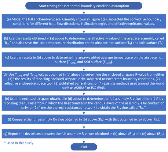
Figure 2.
General Procedure for investigating the effect of using isothermal boundary conditions for enclosed airspaces on the effective R-value of the full enclosed airspace assemblies shown in Figure 1a.
The R-value obtained for the enclosed airspace from step (d), along with the dimensions and thermal conductivities of various layers shown in Figure 1a, are used to determine the overall R-value of the reflective building assembly, referred to as “R2a”, either by modeling the reflective building assembly in which the mode of heat transfer in all layers is achieved via conduction, or by using the thermal resistances network of all layers (step (e) in Figure 2). When the difference between the two R-values of R1a and R2a is small, the isothermal conditions assumption needed to determine the R-value of reflective enclosed airspace in the building component is then considered an acceptable assumption.
A study of the assumption of isothermal conditions for “enclosed airspaces only” of different orientations, subjected to various heat-flow directions (see Figure 1b) is completed. The procedure used in this case is described in Figure 3. In this case, the R-values of the enclosed airspaces are determined using the validated numerical model when they are subjected to convective boundary conditions on both a hot surface and a cold surface. The obtained R-values are called “R1b” (step (a) and (b) in Figure 3). Additionally, the surface temperature distributions on both the hot surface (TH) and the cold surface (TC) from the numerical simulations are used to determine the area-weighted average temperatures for both the hot surface (TH,avg) and the cold surface (TC,avg). Then, the obtained average temperatures of both hot and cold surfaces (TH,avg and TC,avg) are used by the numerical model to re-determine the R-values of the enclosed airspaces under the assumption of isothermal boundary conditions (i.e., “R2b”). Similar to the reflective building assembly, when the difference between the two R-values of R1a and R2a for enclosed airspace only (Figure 1b) is small, the isothermal conditions assumption for determining the R-value of reflective enclosed airspace is an acceptable assumption (see Figure 3). As the low-emittance (low-e) foils/coatings used in reflective airspace surfaces can be increased due to dust accumulation or contamination on these surfaces, the procedures provided in Figure 2 and Figure 3 were completed for effective emittances from 0 to 0.82.
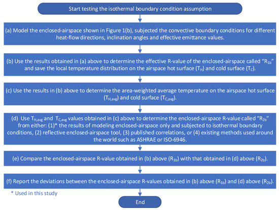
Figure 3.
General procedure for investigating the effect of using isothermal boundary conditions for enclosed airspaces on the effective R-value of the enclosed airspace shown in Figure 1b.
5. Results and Discussion
This section discusses the effect of radiative heat exchange at the ends (or edges) of the enclosed airspace on the calculated R-values of reflective building assemblies with different heat-flow directions. The results obtained using convective boundary conditions and isothermal boundary conditions are compared. Finally, the impact of the airspace aspect ratio on the R-value of the enclosed reflective airspace is also discussed.
5.1. Effect of Radiative Heat Exchange at Airspace Edges
The present model accounts for heat transfer by radiation on all surfaces that bound the enclosed reflective airspaces. For the reflective building assembly shown in Figure 1a, numerical simulations were completed to show the effect of accounting for heat transfer by radiation at the edges of the airspace with emittance of E3. Low-emittance surfaces used in reflective insulation materials have emittance less than 0.1 [28]. Contamination, water vapor condensation or dust accumulation on low-e surfaces, however, would result in elevated surface emittance [35]. Numerical simulations, therefore, were completed to cover effective emittances (E) from 0 to 0.82, where the effective emittance is given as [25,36]:
where E2 is equal 0.9 [24] and a wide range of E1 from 0–0.9 was used to cover various building applications. Note that when the values of E1 = 0.9 and E2 = 0.9, the resulting value of the effective emittance E Equation (1) is 0.82. At the edges of the airspace, two cases for the emittance E3 were considered:
E = 1/[1/E1 + 1/E2 − 1],
- No radiation takes place at the two ends of airspace surfaces (i.e., E3 = 0.0). This case is called “without end (or edge) effect”, which represents the case of net radiative transport between two large/infinite parallel surfaces that is currently being used in ISO 6946 [23] and ASHRAE [24,25]. The surfaces of the two ends of the airspace are usually the surfaces of the framing (e.g., furring or spacers) that bound the airspace. Note that the case of without end effect would represent the situation in which low-e material is present on the surfaces of the framing/spacers facing the airspace. It is important to point out that the main reason for addressing this case is to explore the impact on R-value due to installing low-e foil or coating on the surfaces of the framing/spacers that face the airspace and are parallel to the heat-flow direction, which is of interest to reflective insulation manufacturers, building authorities and designers.
- Radiation takes place at the two ends of the airspace surfaces at E3 = 0.9 [24]. This case is called “with end effect”.
For the case of vertical assembly (θ = 90°) subjected to horizontal heat flow, Figure 4 shows the effect of radiation at the two ends of the 50.8 mm airspace on the R-value. For the case without end effect (E3 = 0.0) at a given effective emittance value, the net rate of heat transfer due to the radiative exchange on all airspace surfaces is smaller than that for the case with end effect (E3 = 0.9). As such, the R-value for the case without end effect is larger than that for the case with the end, as shown in Figure 4. For the case without end effect, increasing the effective emittance from 0 to 0.82 decreases the R-value of the building assembly from 1.248 m2·K/W to 0.984 m2·K/W—a 26.9% reduction. For the case with the end effect, however, increasing the effective emittance from 0 to 0.82 decreases the R-value from 1.225 m2·K/W to 0.982 m2·K/W, a 24.8% reduction in the R-value of the building assembly. Furthermore, the percentage overestimate in the R-value due to neglecting the end effect (plotted on the right y-axis of Figure 4) reaches its highest value (1.9%) at the lowest value of effective emittance (i.e., E = 0.0); whereas this percentages reaches its lowest value (0.2%) at the highest value of effective emittance (0.82). For E > 0.3, Figure 4 shows that the difference in R-values decreases from 0.6% to 0.2% as E increases from 0.3 to 0.82. For E < 0.3, however, the difference in the R-value increases from 0.6% to 1.9% as E decreases from 0.3 to 0.0. For E = 0.03, the R-value without end effect is 1.226 m2·K/W and the R-value with the end effect is 1.205 m2·K/W—a difference of 1.7%.
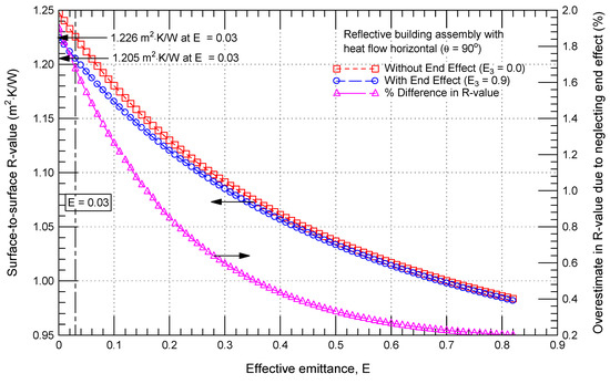
Figure 4.
Effect of accounting for heat transfer by radiation at the two ends of the airspace subjected to horizontal heat flow for the case of reflective building assembly shown in Figure 1a (θ = 90°).
For a horizontal reflective building assembly (θ = 0°) with upward heat flow or downward heat flow, Figure 5a and Figure 5b, respectively, show the effect on the R-value of heat transfer by radiation on the airspace ends. As shown in these figures, for the case without an end effect, increasing E from 0.0 to 0.82 results in the R-value decreasing from 1.170 to 0.973 m2·K/W for upward heat flow and from 2.494 to 1.078 m2·K/W, which represents a reduction in the R-value of the building assembly by 20.2% for upward heat flow and 131.3% for downward heat flow (versus 26.9% for vertical assembly with horizontal heat flow). Additionally, for the case with end effect, increasing E from 0.0 to 0.82 has resulted in the R-value decreasing from 1.147 to 0.970 m2·K/W for upward heat flow and from 2.200 to 1.073 m2·K/W for downward heat flow, which represents an 18.2% reduction in R-value of the building assembly for upward heat flow and a 105.0% reduction for downward heat flow (versus 24.8% for vertical assembly with horizontal heat flow).
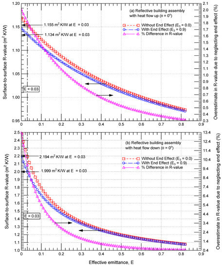
Figure 5.
Effect of accounting for heat transfer by radiation at the two ends of the airspace subjected to heat flow (a) up and (b) down for the case of reflective building assembly shown in Figure 1a (θ = 0°).
As indicated earlier for the same effective emittance, the net rate of heat transfer by radiation for the case without end effect is lower than that for the case with end effect. This has resulted in a higher R-value for the former than that for the latter, as shown in Figure 5. Figure 5a,b show that the heat transferred by radiation on the ends has an insignificant effect on the R-value for effective emittance greater than 0.5 for upward heat flow (difference in R-values decreases from 0.5% at E = 0.5 to 0.3% at E = 0.82, Figure 5a), and 0.3 for downward heat flow (difference in R-values decreases from 1.7% at E = 0.3 to 0.4% at E = 0.82). At low values of E (E < 0.5 for upward heat flow and E < 0.3 for heat flow), the difference in R-value without end effect and with end effect increases at a higher rate (in relation to high E values) as E decreases. For upward heat flow, the difference in the R-value increases from 0.5% at E = 0.5 to 2.0% at E = 0.0. However, for downward heat flow, the difference in R-value increases from 1.7% at E = 0.3 to 13.3% at E = 0.0. Finally, at an effective emittance of 0.03 for reflective building assemblies with upward heat flow (Figure 5a), the case without the end effect overestimated the R-value (1.155 m2·K/W) by 1.9% in comparison with the case with end effect (1.134 m2·K/W). Additionally, at E = 0.03 and downward heat flow (Figure 5b), the case without end effect overestimated the R-value (2.194 m2·K/W) by 9.8% in comparison with the case with the end effect (1.999 m2·K/W).
For sloped reflective building assemblies (θ = 45°), Figure 6a and Figure 6b, respectively, show the effect of accounting for the heat transfer by radiation on the ends of the airspace on R-value for reflective building assembly subjected to upward heat flow and downward heat flow. As shown in these figures, the trends of the R-values for the full range of E with and without end effects are similar to the previous cases of horizontal heat flow (θ = 90°, Figure 4) and upward and downward heat flow (θ = 0°, Figure 5a,b). At E = 0.03, the R-value without end effect (1.235 m2·K/W) is overestimated by 1.6% in comparison to the case with the end effect (1.215 m2·K/W) for sloped reflective assemblies with upward heat flow (Figure 6a). Additionally, at E = 0.03, the R-value without the end effect (1.294 m2·K/W) is overestimated by 2.2% in comparison to the case with the end effect (1.266 m2·K/W) for sloped reflective assemblies with downward heat flow (Figure 6b).
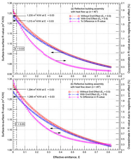
Figure 6.
Effect of accounting for heat transfer by radiation at the two ends of the airspace subjected to heat flow (a) up and (b) down for the case of reflective building assembly shown in Figure 1a (θ = 45°).
As indicated earlier, the ends of the enclosed airspace represent the surfaces of the spacers/framing for double glazing systems and surfaces of the furring in the furred airspace assemblies for wall and roofing systems. As shown in Figure 1a, the length of the airspace ends in this discussion is 50.8 mm and its length is 406.4 mm. It is anticipated that the effect of radiative heat exchange on the airspace ends on the R-value would be greater for longer airspace ends and shorter airspace length. For example, in a previous study [33] for airspace ends of 88.9 mm (versus 50.8 mm in this study) and airspace length of 406.4 mm (same as this study), the radiative heat exchange on the airspace ends has a greater effect on the R-value than that in this study. The case without end effect represents the situation in which low-e foil or coating is present on the surfaces of the framing that faces the airspace. The difference in the R-value for the case without end effect and that with the end effect provides the potential increase in the R-value due to the installation of low-e foil or coating on the framing of enclosed airspaces.
In closing, the R-values in Figure 4 through Figure 6 show that the neglect of thermal radiation to the ends (or edges) of the enclosed reflective airspace results in an overestimate of the surface-to-surface R-value for the building assembly that was modeled for the five heat-flow directions. Approximate maximum percentage overestimates are contained in Table 1. This table shows that the percentage overestimates increase as the heat-flow direction changes from upward heat flow to downward heat flow. The overestimate becomes large as the heat flows downward, since radiation dominates for downward heat transfer in many practical applications.

Table 1.
Maximum overestimated values in the surface-to-surface assembly R-values due to neglecting the radiative exchange on the airspace ends (or edges).
5.2. Test the Assumption of Isothermal Boundary Conditions
To test the impact of the isothermal boundary assumptions for reflective building assemblies (Figure 1a) of different inclination angles (θ) on the R-values, results for five orientations, namely: (1) heat follow up at θ of 0° (i.e., horizontal orientation), (2) downward heat flow at θ of 0°, (3) horizontal heat flow at θ of 90° (i.e., vertical orientation), (4) heat follow-up at θ of 45° and (5) downward heat flow at θ of 45° have been computed. As shown in Figure 1a, the reflective building assemblies consisted of 12.7 mm-thick gypsum board and a 25.4 mm-thick layer of EPS separated by 38.1 mm-thick wood studs to form an enclosed airspace of 50.8 mm thickness and 406.4 mm width. The thermal conductivity of the various layers used in the numerical simulations is provided in this figure. Additionally, the impact of the assumption of isothermal conditions on the R-values was calculated for the enclosed reflective airspaces shown in Figure 1b for cases 1 to 5 listed above. In all cases, results are obtained for the convective boundary condition on the hot surface with h1 = 12 W/(m2·K) and T∞1 = 20 °C, and the convective boundary condition on the cold surface with h2 = 8 W/(m2·K) and T∞2 = −20 °C.
For a given operating condition in the case of absence of heat transfer by convection at an effective emittance E = 0, the heat transfer inside the airspace occurs via conduction only. Increasing the value of the effective emittance results in an increase in the rate of heat transfer by radiation, and thus a decrease in the R-value. For a given value of the effective emittance in this case (i.e., absence of convection), the R-values of the building assembly shown in Figure 1 are the same for all heat flow directions and inclination angles. However, by accounting for heat transfer via convection, both airflow velocity and the shapes and number of convection loops inside the airspace of the building assembly strongly depend on both the heat flow direction and the inclination angle. As shown in subsequent subsections, higher airflow velocity and a larger number of convection loops would increase the rate of heat transfer by convection, subsequently decreasing the R-value.
5.2.1. Upward Heat Flow for θ = 0°
Due to the temperature difference across the reflective building assembly, a buoyancy driven flow is developed in the enclosed airspace, resulting in either mono-cellular or multi-cellular airflow with a varying number of convective loops. The temperature and airflow velocity distributions and the resulting number of convection loops depend on both the orientation of the reflective building assembly and the direction of the heat flowing through the assembly. For the horizontal reflective building assembly shown in Figure 1a, subjected to convective boundary conditions with upward heat flow (e.g., roof applications in cold climates) at E = 0.05, Figure 7 shows the temperature distribution in the whole assembly (Figure 7a), temperature distribution in the airspace only (Figure 7b) and the resultant air velocity distribution in the airspace (Figure 7c). To show the details of the temperature distribution, different contour levels were used for the whole assembly and the airspace. As shown in this figure, the highest and lowest temperatures in the whole assembly are 18.2 °C and −16.7 °C, respectively (Figure 7b), whereas the highest and lowest temperatures in the enclosed airspace are 16.6 °C and −1.18 °C, respectively (Figure 7b). Figure 7 shows that six convection loops were formed inside the airspace where the highest resultant air velocity is 73.6 mm/s.
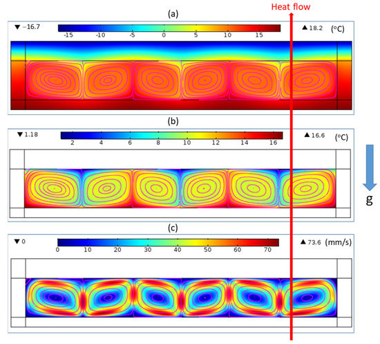
Figure 7.
Velocity streamline for upward heat flow at effective emittance of 0.05: (a) temperature distribution in the reflective building assembly, (b) temperature distribution in the airspace only, and, (c) resultant air velocity distribution in the airspace (inclination angle of 0°).
Figure 8a and b, respectively, show the temperature distributions on the airspace cold surface and hot surface for E = 0.05, 0.2, 0.5 and 0.82. As shown in these figures, the shapes of these temperature distributions depend on E, the number of convection loops and airflow velocity inside the enclosed airspace. The values of the temperatures on the airspace cold surface at E of 0.05 are the lowest and those at E of 0.82 are the highest (Figure 8a). Conversely, the values of the temperature on the airspace hot surface at E of 0.05 are the highest and those at E of 0.82 are the lowest (Figure 8a).
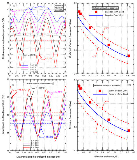
Figure 8.
Airspace temperature distributions on the cold top surface (a) and the hot bottom surface (b), and the surface-to-surface R-values (c) and the air-to-air R-values (d) for reflective building assemblies with convective boundary conditions shown in Figure 1a for the case of upward heat flow (inclination angle of 0°).
For E = 0.05, 0.2, 0.5 and 0.82, the area-weighted average temperatures on the airspace cold surface (TC,avg) and hot surface (TH,avg) are given by the dashed horizontal lines in Figure 8a and b, respectively. The values of TC,avg are 5.22 °C, 6.35 °C, 7.92 °C and 9.02 °C, and the corresponding values of TH,avg are 15.13 °C, 14.96 °C, 14.71 °C and 14.53 °C. To investigate the impact of the isothermal boundary conditions assumption on the R-value, the values of TC,avg and TH,avg are applied to the airspace cold surface and hot surface, as described earlier, and the procedure provided in Figure 2 is followed. Figure 8c shows a comparison between the surface-to-surface R-value based on the convective boundary conditions with those based on the isothermal boundary conditions for a wide range of E. As shown in this figure, the maximum deviation between the surface-to-surface R-values based on the convective and isothermal boundary conditions is ±3%. By including the contributions of the film coefficients (i.e., h1 and h2; see Figure 1a) on the external hot surface and the cold surface of the reflective building assembly, Figure 8d shows that the maximum deviation between the air-to-air R-values based on both the convective and isothermal boundary conditions is also ±3%.
For horizontal enclosed airspaces with upward heat flow (see Figure 1b) with convective boundary conditions, Figure 9a and b, respectively, show the temperature distributions on the cold surface and hot surface at E = 0.05, 0.2, 0.5 and 0.82. The highest local temperature on the cold surface for the case of enclosed airspace only (Figure 1b) occurs at E of 0.82 and the lowest local temperature occurs at E of 0.05 (Figure 9a); whereas the highest local temperature on the hot surface occurs at E of 0.05 and the lowest local temperature occurs at E of 0.82 (Figure 9b). At E = 0.05, the maximum difference in the local temperatures on the airspace cold surface ΔTC,max is 10.84 °C (Figure 9a); whereas the maximum difference in the local temperatures on the airspace hot surface ΔTH,max is 7.35 °C (Figure 9b). At E of 0.05, 0.2, 0.5 and 0.82, respectively, the area-weighted average temperatures on the airspace cold surface TC,avg are −9.89 °C, −8.98 °C, −7.49 °C and −6.25 °C (Figure 9a), and the area-weighted average temperatures on the hot surface TH,avg are 13.26 °C, 12.65 °C, 11.66 °C and 10.83 °C. Using the instructions shown in Figure 3 for a given E, the values of TC,avg and TH,avg are used as boundary conditions on the airspace cold surface and the hot surface to determine the R-value of the enclosed airspace (i.e., under the assumption of isothermal boundary conditions). For a wide range of effective emittance for the case of enclosed airspace only, Figure 9c shows that the maximum deviation between the surface-to-surface R-values based on convective and isothermal boundary conditions is ±3%. Furthermore, the maximum deviation between the air-to-air R-values based on convective and isothermal boundary conditions is ±3% (Figure 9d).
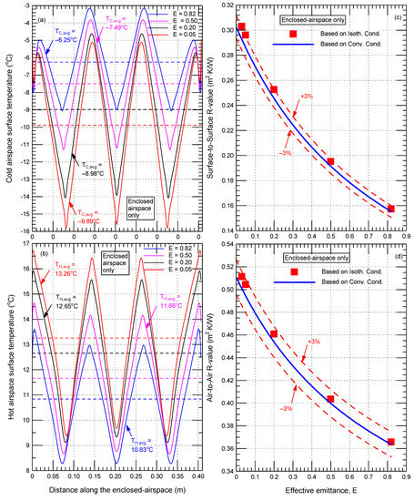
Figure 9.
Airspace temperature distributions on the cold top surface (a) and the hot bottom surface (b), and the surface-to-surface R-values (c) and the air-to-air R-values (d) for reflective enclosed airspaces with convective boundary conditions shown in Figure 1b for the case of upward heat flow (inclination angle of 0°).
5.2.2. Downward Heat Flow for θ = 0°
For the horizontal reflective building assembly (θ = 0°) shown in Figure 1a with downward heat flow (e.g., roof application in hot climates) and subjected to convective boundary conditions at E = 0.05, Figure 10a, b and c, respectively, show the temperature distribution in the whole assembly, the temperature distribution in the airspace and the resultant air velocity inside the airspace. As shown in this figure, relatively stable air stratification occurred in the airspace, which can be observed in the shape of the temperature distributions; convection loops formed inside the airspace with quite small air velocity in relation to reflective building assembly with upward heat flow. For example, the maximum resultant air velocity for the assembly with downward heat flow (15.7 mm/s, Figure 10) is only 1/5 of that for the upward heat flow (73.5 mm/s, Figure 7c). As a result, the reduction in the R-value due to heat transfer by convection with downward heat flow is much smaller than that for upward heat flow. As such, for the same value of effective emittance, the R-value for the assembly with downward heat flow (Figure 11c,d) is much higher than that for the assembly with upward heat flow (Figure 8c,d). For example, at E of 0.05, the surface-to-surface R-value for the assembly with downward heat flow subjected to convective boundary conditions (1.893 m2·K/W) is 68% higher than that with upward heat flow (1.125 m2·K/W).
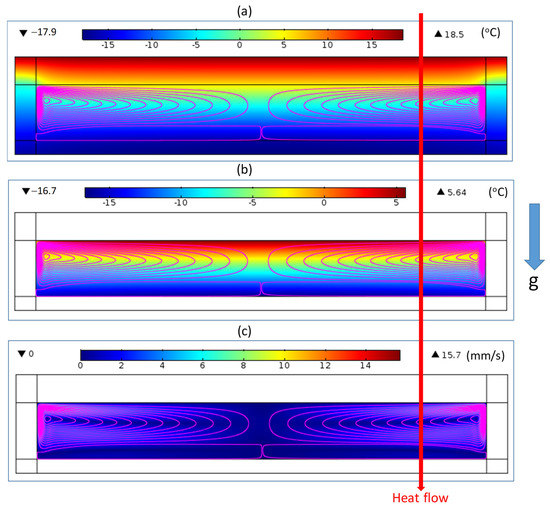
Figure 10.
Velocity streamline for downward heat flow at effective emittance of 0.05: (a) temperature distribution in the reflective building assembly, (b) temperature distribution in the airspace only, and, (c) resultant velocity distribution in the airspace (θ = 0°).
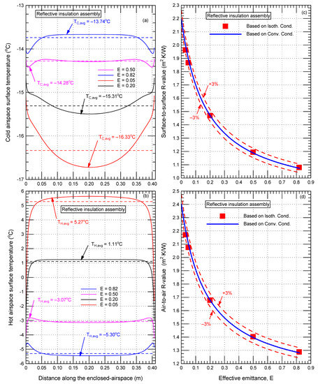
Figure 11.
Airspace temperature distributions on the cold bottom surface (a) and the hot top surface (b), and the surface-to-surface R-values (c) and the air-to-air R-values (d) of horizontal reflective building assembly with convective boundary conditions shown in Figure 1a for downward heat flow (inclination angle of 0°).
Figure 11a,b show the temperature distributions, as well as the area-weighted average temperatures on the airspace cold surface and hot surface, respectively. At E = 0.05, 0.2, 0.5 and 0.82, respectively, the values of TC,avg are −16.33 °C, −15.31 °C, −14.28 °C and −13.74 °C (Figure 11a), and the values of TH,avg are 5.27 °C, 1.11°C, −3.07 °C and −5.30 °C (Figure 11b). As per the procedure provided in Figure 2, these values for TC,avg and TH,avg are used as isothermal boundary conditions on the airspace cold surface and hot surface to obtain the airspace R-value. For a wide range of effective emittance values, Figure 11c shows a comparison between the surface-to-surface R-value based on the convective boundary conditions with that based on the isothermal boundary conditions in which the maximum deviation between the surface-to-surface R-values based on both convective and isothermal boundary conditions is ±3%. Additionally, Figure 11d shows that the maximum deviation between the air-to-air R-values based on both the convective and isothermal boundary conditions is also ±3%.
For the enclosed airspace shown in Figure 1b with downward heat flow and subjected to convective boundary conditions on the cold surface and hot surface, Figure 12a,b show the temperature distributions and the area-weighted average temperature on the cold surface and hot surface, respectively. For E = 0.05, 0.2, 0.5 and 0.82, respectively, the values of TC,avg are −16.36 °C, −14.27 °C, −11.18 °C and −8.90 °C (Figure 12a), and the values of TH,avg are 17.57 °C, 16.18 °C, 14.12 °C and 12.60 °C (Figure 12b). Similar to the reflective building assembly (Figure 1a), the R-value for the case of reflective airspace with downward heat flow (Figure 1b) is significantly higher than that with upward heat flow. As an example, at E of 0.05, the surface-to-surface R-value for reflective airspace subjected to convective boundary conditions with downward heat flow (1.166 m2·K/W, Figure 12c) is 309% higher than that with upward heat flow (0.285 m2·K/W, Figure 9c). As per the procedure shown in Figure 3, the values of TC,avg and TH,avg are used as isothermal boundary conditions on the airspace cold surface and the hot surface to determine the airspace R-values. For a wide range of effective emittance, Figure 12c,d show that the maximum deviation in the surface-to-surface R-values and air-to-air R-values based on convective and isothermal boundary conditions is ±3%.
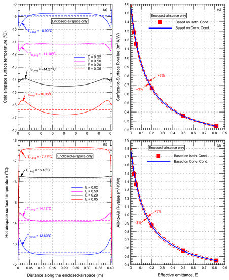
Figure 12.
Airspace temperature distributions on the cold bottom surface (a) and the hot top surface (b), and the surface-to-surface R-values (c) and the air-to-air R-values (d) of horizontal enclosed airspace with convective boundary conditions shown in Figure 1b for downward heat flow (inclination angle of 0°).
5.2.3. Horizontal Heat Flow for θ = 90°
For the vertical reflective building assembly (θ = 90°) shown in Figure 1a (rotated 90°) with horizontal heat flow and subjected to convective boundary conditions, Figure 13a–c show the temperature distribution in the whole assembly, the temperature distribution in the airspace and the resultant air velocity in the airspace, respectively. As shown in these figures, the buoyancy driven flow has resulted in developing one convective loop in which the highest resultant air velocity is 86.9 mm/s. The one convection loop in the airspace causes large variations in the local temperatures on both the airspace cold side (Figure 14a) and hot surface (Figure 14b). The temperature variation along the airspace cold surface and hot surface depends on the value of the effective emittance. For example, the maximum temperature difference on the cold surface ΔTC,max at E of 0.05 is 11.24 °C, whereas that at E of 0.82 is 4.48 °C (Figure 14a). Additionally, the maximum temperature difference on the hot surface ΔTH,max at E of 0.05 is 5.11 °C, whereas that at E of 0.82 is 2.75 °C (Figure 14b). At E of 0.05, 0.2, 0.5 and 0.82, the local temperatures on the airspace cold surface shown in Figure 14a were used to determine the area-weighted average temperatures TC,avg, which are 4.07 °C, 5.51 °C, 7.45 °C and 8.74 °C, respectively. At these values of effective emittance, the local temperatures on the airspace hot surface shown in Figure 14b were also used to determine the area-weighted average temperatures TH,avg, which are 15.48 °C, 15.21 °C, 14.86 °C and 14.63 °C, respectively.
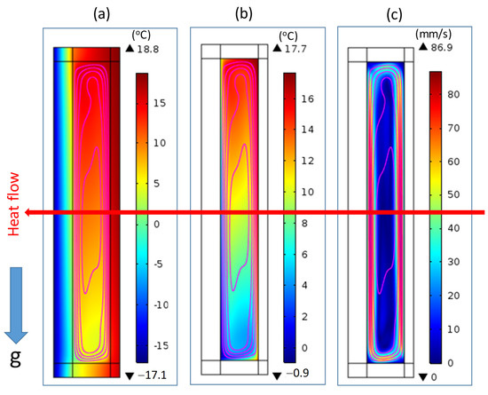
Figure 13.
Velocity streamline for horizontal heat flow at effective emittance of 0.05: (a) temperature distribution in the reflective building assembly, (b) temperature distribution in the airspace only and, (c) resultant air velocity distribution in the airspace (inclination angle of 90°).
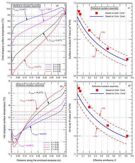
Figure 14.
Airspace temperature distributions on the cold left surface (a) and the hot right surface (b), and the surface-to-surface R-values (c) and the air-to-air R-values (d) of vertical reflective building assemblies with convective boundary conditions shown in Figure 1a for horizontal heat flow (inclination angle of 90°).
Similar to the horizontal reflective building assembly with upward heat flow and down, the values of TC,avg and TH,avg provided above for the reflective building assembly with horizontal heat flow were used as isothermal boundary conditions to determine the airspace R-values (see the procedure in Figure 2). Figure 14c and d, respectively, show comparisons for the surface-to-surface R-values and air-to-air R-values based on the convective and isothermal boundary conditions. As shown in these figures, the maximum deviation on the R-values based on both convective and isothermal boundary conditions is ±3%.
For the vertical enclosed airspace of various effective emittance shown in Figure 1b (rotated 90°) with horizontal heat flow and subjected to convective boundary conditions, Figure 15a,b show the local temperature distribution on the airspace cold surface and hot surface, respectively. For the cold surface, the maximum temperature difference ΔTC,max at E of 0.05 is 15.51 °C and that at E of 0.82 is 8.12 °C (Figure 15a). Additionally, for the airspace hot surface, the maximum temperature difference ΔTH,max at E of 0.05 is 8.78 °C and that at E of 0.82 is 6.29 °C (Figure 15b). For the airspace cold surface at E of 0.05, 0.2, 0.5 and 0.82, the values of TC,avg are −11.17 °C, −10.08 °C, −8.31 °C and −6.86 °C, respectively. Additionally, for the airspace hot surface at these values of E, the values of TH,avg are 14.11 °C, 13.39 °C, 12.20 °C and 11.24 °C, respectively. As per the procedure shown in Figure 3, the values of TC,avg and TH,avg were used as isothermal conditions to determine the airspace R-values. For a wide range of effective emittance, Figure 15c for the surface-to-surface R-values and Figure 15d for the air-to-air R-values show that the maximum deviation in these R-values based on both the convective and isothermal boundary conditions is ±3%.
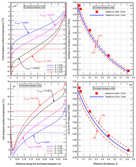
Figure 15.
Airspace temperature distributions on the cold left surface (a) and hot right surface (b), and the surface-to-surface R-values (c) and the air-to-air R-values (d) of vertical enclosed airspaces with convective boundary conditions shown in Figure 1b for horizontal heat flow (inclination angle of 90°).
5.2.4. Upward and Downward Heat Flow and for Sloped Orientation for θ = 45°
For sloped roof applications, numerical simulations were completed for the reflective building assembly shown in Figure 1a (rotated 45°) with upward heat flow (i.e., cold climate) and subjected to convective boundary conditions. At E = 0.05, Figure 16a, b and c, respectively, show the temperature distributions in the whole assembly, the temperature distribution in the airspace and the resultant air velocity where one convection loop was formed in the airspace in which the highest resultant air velocity is 85 mm/s. For the same reflective building assembly subjected to convective boundary conditions at E = 0.05 but with downward heat flow (i.e., hot climate), the corresponding results are shown in Figure 17a–c where one convection loop was also formed in the airspace in which the highest resultant air velocity (68.8 mm/s) was 19% lower than that for upward heat flow (85 mm/s). For the case with upward heat flow, Figure 18a and b, respectively, show the local temperature distributions on the airspace cold surface and hot surface at effective emittances of 0.05, 0.2, 0.5 and 0.82. The corresponding results for the case with downward heat flow are shown in Figure 19a,b.
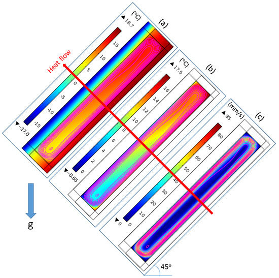
Figure 16.
Velocity streamline for upward heat flow at effective emittance of 0.05: (a) temperature distribution in the reflective building assembly, (b) temperature distribution in the airspace only and, (c) resultant air velocity distribution in the airspace (inclination angle of 45°).
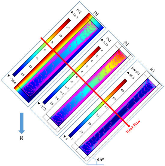
Figure 17.
Velocity streamline for downward heat flow at effective emittance of 0.05: (a) temperature distribution in the reflective building assembly, (b) temperature distribution in the airspace and, (c) resultant velocity distribution in the airspace (θ = 45°).
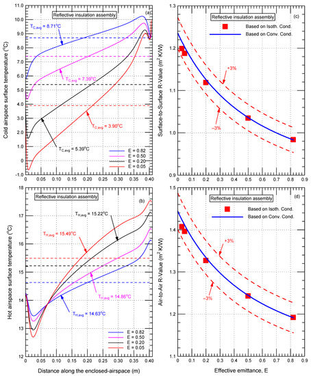
Figure 18.
Airspace temperature distributions on the cold top surface (a) and the hot bottom surface (b), and the surface-surface R-values (c) and the air-to-air R-values (d) of 45° reflective building assembly subjected to convective boundary conditions shown in Figure 1a for upward heat flow.
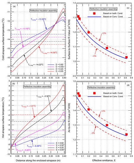
Figure 19.
Airspace temperature distributions on the cold bottom surface (a) and the hot top surface (b), and the surface-to-surface R-values (c) and the air-to-air R-values (d) of 45° reflective building assembly with convective boundary conditions shown in Figure 1a for downward heat flow.
Like the vertical assembly with horizontal heat flow, and horizontal assembly with upward and downward heat flow, the shapes of the local temperatures on the airspace cold surface and hot surface for sloped assemblies with upward heat flow and downward heat flow depend on E. As examples for the case with upward heat flow, the maximum temperature difference on the airspace cold surface ΔTC,max at E of 0.05 is 10.58 °C versus 4.39 °C at E of 0.82 (Figure 18a). The corresponding value of ΔTC,max for the case with downward heat flow is 6.90 °C at E of 0.05 versus 3.61 °C at E of 0.82 (Figure 19a). Additionally, for the case with upward heat flow, the maximum temperature difference on the airspace hot surface ΔTH,max at E of 0.05 is 4.85 °C versus 2.69 °C for E of 0.82 (Figure 18b). The corresponding value of ΔTH,max for the case with downward heat flow is 13.89 °C for E of 0.05 versus 5.32 °C for E of 0.82 (Figure 19b).
The airspace temperature distributions on the cold surface and hot surface were used to determine the area-weighted average temperatures TC,avg and TH,avg. For upward heat flow at E = 0.05. 0.2, 0.5 and 0.82, the values for TC,avg are 3.90 °C, 5.39 °C, 7.39 °C and 8.71 °C (Figure 18a) and those for TH,avg are 15.49 °C, 15.22 °C, 14.86 °C and 14.63 °C (Figure 18b). For the case of downward heat flow, the corresponding values for TC,avg are −14.56 °C, −14.22 °C, −13.76 °C and −13.35 °C (Figure 19a), and those for TH,avg are −1.91 °C, −3.30 °C, −5.20 °C and −6.49 °C (Figure 19b). As demonstrated in Figure 2, the values of TC,avg and TH,avg were used as isothermal boundary conditions on the airspace surfaces to determine the airspace R-values.
As indicated earlier, the airflow velocity in the airspace for the assembly with downward heat flow is lower than that for the assembly with upward heat flow, where the highest resultant velocity at E = 0.05 in the former (68.8 mm/s, Figure 17c) is 19% lower than that in the latter (85 mm/s, Figure 16c). Consequently, at a given effective emittance, this would result in a reduction in the R-value due to heat transfer by convection for the assembly, with a downward heat flow smaller than that for the assembly with upward heat flow. As such, the R-value of the assembly with downward heat flow (see Figure 19c,d) is greater than that of the assembly with upward heat flow (see Figure 18c,d). At E = 0.05, as an example, the surface-to-surface R-value for the assembly subjected to convective boundary conditions with downward heat flow (1.252 m2·K/W, Figure 19c) is 4% greater than that for the assembly with upward heat flow (1.203 m2·K/W, Figure 18c). For the surface-to-surface R-values and air-to-air R-values over a wide range of effective emittance, Figure 18c,d (assembly with upward heat flow) and Figure 19c,d (assembly with downward heat flow) show that the maximum deviation in these R-values based on both the convective and isothermal boundary conditions is ±3%.
Finally, for the reflective enclosed airspace shown in Figure 1b (rotated 45°) with upward heat flow and subjected to convective boundary conditions, Figure 20a and Figure 20b, respectively, show the local temperature distributions on the airspace cold surface and hot surface. The corresponding results for the reflective enclosed airspace subjected to convective boundary conditions with downward heat flow are shown in Figure 21a,b. For upward heat flow at E of 0.05 and 0.82, respectively, Figure 20a shows that the highest temperature difference on the airspace cold surface ΔTC,max is 13.10 °C and 7.26 °C (versus 12.28 °C and 8.39 °C for downward heat flow; Figure 21a). Additionally, for downward heat flow at E of 0.05 and 0.82, respectively, Figure 20b shows that the highest temperature difference on the airspace hot surface ΔTH,max is 8.10 °C and 5.97 °C (versus 13.26 °C and 6.61 °C for downward heat flow, Figure 21b). For a wide range of E, the surface-to-surface and air-to-air R-values are provided in Figure 20c,d for the airspace with upward heat flow and Figure 21c,d for airspace with downward heat flow. At E = 0.05, the surface-to-surface R-value of the enclosed airspace subjected to convective boundary conditions with downward heat flow (0.417 m2·K/W, Figure 21c) is 32% higher than that with upward heat flow (0.317 m2·K/W, Figure 20c).
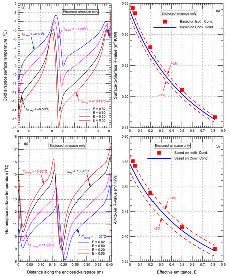
Figure 20.
Airspace temperature distributions on the cold top surface (a) and the hot bottom surface (b), and the surface-to-surface R-values (c) and the air-to-air R-values (d) for 45° enclosed airspace with convective boundary conditions shown Figure 1b for upward heat flow.
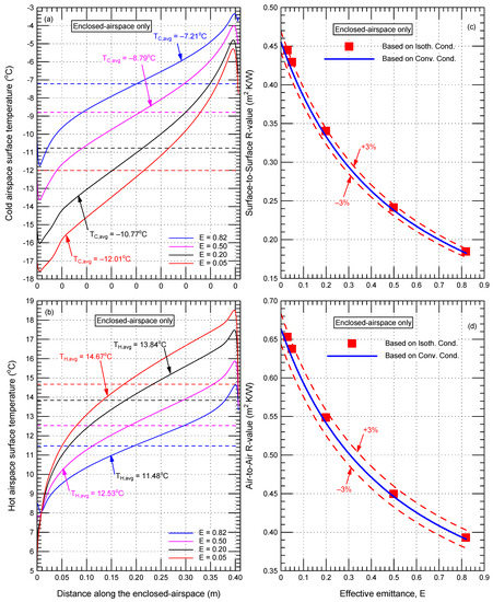
Figure 21.
Airspace temperature distributions on the cold bottom surface (a) and the hot top surface (b), and the surface-to-surface R-values (c) and the air-to-air R-values (d) for the 45° enclosed airspace with convective boundary conditions shown in Figure 1b for downward heat flow.
For the enclosed airspace (Figure 1b) with upward heat flow at E = 0.05, 0.2, 0.5 and 0.82, respectively, Figure 20a shows that the area-weighted average temperature on the airspace cold surface TC,avg is −10.49 °C, −9.50 °C, −7.88 °C and −6.53 °C (versus −12.01 °C, −10.77 °C, −8.79 °C and −7.21 °C for downward heat flow, Figure 21a), whereas the area-weighted average temperature on the airspace hot surface TH,avg shown in Figure 20b is 13.66 °C, 13.00 °C, 11.92 °C and 11.02 °C (versus 14.67 °C, 13.84 °C, 12.53 °C and 11.48 °C for downward heat flow, Figure 21b). These values for TC,avg and TH,avg were used as isothermal boundary conditions on the airspace cold surface and hot surface to determine the airspace R-value using Figure 3. As shown in Figure 20c,d for the airspace with upward heat flow and Figure 21c,d for the airspace with downward heat flow, the maximum deviation between the surface-to-surface and air-to-air R-values based on both convective and isothermal boundary conditions is ±3%.
In summary, the results provided in this subsection showed that using the actual boundary conditions (convective boundary conditions in this study) to determine the R-values of building assemblies with reflective insulations or enclosed airspaces have resulted in non-uniform local temperature distributions on both the airspace cold and hot surfaces, where the non-uniformity/shapes of these temperature distributions strongly depend on: (a) effective emittance, (b) orientation and (c) heat-flow direction. However, to the best of our knowledge, all available methods, tables, correlations and tools that are currently being used around the world to determine the R-values of enclosed airspace are based on isothermal boundary conditions (i.e., constant temperature on the airspace cold surface, TC, and constant temperature on the airspace hot surface, TH). For all cases presented in this subsection that include reflective building assembly (Figure 1a) and enclosed airspace (Figure 1b) of various orientations with different heat-flow directions, all comparisons between the surface-to-surface R-values and air-to-air R-values based on both convective and isothermal boundary conditions are summarized in Figure 22a,b for reflective building assembly and Figure 22c,d for enclosed airspace. As shown in Figure 22a through Figure 22d, the maximum deviation between all R-values based on convective boundary conditions and isothermal boundary conditions is ±3%. As such, for the full range of effective emittance (0–0.82), the currently available methods [23,24,25,26], correlations [28] and tools [27] based on the assumption of isothermal boundary conditions can be used with confidence to determine the R-values of enclosed airspaces of various orientations with different heat-flow directions.
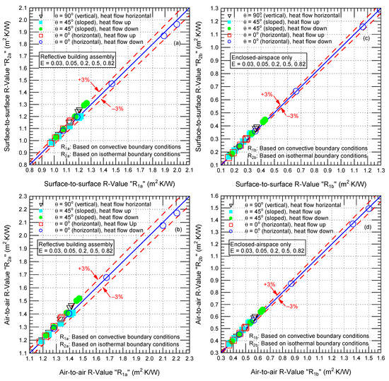
Figure 22.
Based on convective and isothermal boundary conditions for various orientations and heat-flow directions, comparisons of the surface-to-surface R-values (a) and the air-to-air R-values (b) for reflective building assembly shown in Figure 1a, and the surface-to-surface R-values (c) and the air-to-air R-values (d) for enclosed airspace shown in Figure 1b.
5.3. Effect of Airspace Aspect Ratio on R-Value
The ratio of the airspace length, H (perpendicular to the heat-flow direction) to airspace thickness, D (parallel to the heat-flow direction) is defined as the aspect ratio, AR. The effect of AR on the R-values of vertical enclosed airspaces (horizontal heat flow) is discussed in this section. Heat transfer occurs in enclosed airspaces via conduction, convection, and radiation. For the same boundary conditions (TH and TC) and airspace thickness, in the absence of heat transfer in the airspace by convection and radiation, the airspace R-values are independent of AR. However, to show the effect of heat transfer by radiation on the airspace R-values of various aspect ratios, consider the parameter SRL-e, which represents the fraction of low-e airspace surface area of the airspace surface area. SRL-e is the ratio of the surface area of low-e at emittance of E1 to the total surface areas of the enclosed airspace of various emittances (E1, E2 and E3, where E2 = E3 = 0.9 in this study). It follows that SRL-e = 0.5 H/(H + D), which can be rewritten in terms of the aspect ratio (AR = H/D) as SRL-e = 0.5 AR/(AR + 1). SRL-e increases as aspect ratio increases with limiting value of 0.5. In the absence of heat transfer by conduction and convection, and for a given value for low-e E1 or effective emittance E, the larger SRL-e value, which occurs at larger aspect ratio, would result in a reduction in the heat transfer rate in the airspace due to the radiative interchanges on all airspace surfaces. As such, an increase in the aspect ratio (i.e., larger SRL-e) tends to favor an increase in thermal resistance. This observation was tested by modeling the airspace heat transmission with all modes of heat transport included.
Figure 23 contains R-values for E = 0.03, 0.05 and 0.1 for vertical enclosed airspaces (θ = 90°) of various length and thickness 88.9 mm with horizontal heat flow at TH = 90°F and TC = 60°F. Figure 23 also contains R-values for various values of E = 0.03, 0.05 and 0.1, obtained using data from HRP 32 [10,11] and R-values based on ISO 6946 [23]. The R-values based on HRP 32 data or calculated using ISO 6946 have been used around the world for decades to evaluate reflective insulation assemblies. Figure 23 shows the dependence of the R-value on the airspace length (bottom x-axis) and the aspect ratio (top x-axis). As shown in this figure at E of 0.03, 0.05 and 0.1, respectively, the R-values (0.651, 0.606 and 0.516 m2·K/W) of the enclosed airspaces of 2,438.4 mm long (AR = 27.4) are 1.99, 1.90 and 1.72 times that for enclosed airspaces of 101.6 mm long, AR = 1.1 (0.327, 0.319 and 0.300 m2·K/W). The effect of the aspect ratio on the airspace R-value is not accounted for in both HRP 32 and ISO 6946. At these effective emittance values (0.03, 0.05 and 0.1, respectively), the HRP 32 R-values (0.474, 0.445 and 0.409 m2·K/W [10,11]) overestimated the R-values of small aspect ratio of 1.1 by 45%, 40% and 36% and underestimated the R-values of large aspect ratio of 27.4 by 27%, 26% and 21%. Similarly, for these effective emittance values, the ISO 6946 R-values (0.489, 0.462 and 0.407 m2·K/W [23]) overestimated the R-values of small aspect ratio of 1.1 by 50%, 45% and 35% and underestimated the R-values of large aspect ratio of 27.4 by 25%, 24% and 21%.
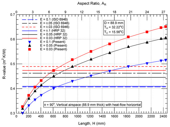
Figure 23.
R-value dependence on aspect ratio for vertical enclosed airspace 88.9 mm thick and subjected to horizontal heat flow with low effective emittance.
6. Conclusions
The neglect of thermal radiative exchange on the airspace surfaces that are parallel to the heat-flow direction (the edges or ends of an enclosed reflective airspace) results in an overestimate of the calculated surface-to-surface building assembly R-value. For the reflective building assembly containing airspace investigated in this study, the results show that:
- The percentage overestimates of the assembly surface-to-surface R-value increase as the heat-flow direction rotates from upward to downward heat flow. The overestimates of the assembly surface-to-surface R-value are below ~2.0% for heat flow from upward to horizontal directions. The percentage estimates increase significantly as heat flow approaches the downward direction, where radiation is dominant.
- The neglect of radiative exchange for heat-flow directions of 45° upward, horizontal, and 45° down impacts the reflective airspace R-values by less than 3% and can be neglected.
- The neglect of radiative exchange with airspace ends impacts the reflective airspace R-values by more than 10%. Consideration should be given to inclusion of radiative exchanges with the airspace ends (edges) for downward heat flow.
The impact of the assumption of isothermal hot surface and cold surface temperatures on surfaces perpendicular to the heat-flow direction was evaluated by comparing the calculated isothermal R-values with R-values obtained with temperature profiles resulting from convection on the hot and cold airspace surfaces. The results show that:
- The use of isothermal airspace surfaces results that are greater than the R-values obtained with convective boundary conditions by less than 3% for effective emittance range from 0 to 0.82 for upward heat flow, 45° up and horizontal. Additionally, the impact of the isothermal assumption for heat flow 45° down and down is negligible for the assemblies modeled.
- The isothermal assumption is valid for the type assemblies that were modeled in this research.
The potential impact of airspace dimensions on calculated R-values was evaluated for a vertically oriented enclosed airspace assembly with horizontal heat flow. The results obtained with numerical modeling were compared with one-dimensional results obtained using ISO 6946 or based on results obtained using data from HRP 32. For the enclosed airspace assembly investigated in this study, the following observations are made.
- The R-values obtained using numerical modeling increase as the aspect ratio increases.
- The R-values obtained using numerical modeling are lower than the one-dimensional results for aspect ratios less than seven.
- The R-values obtained using numerical modeling are greater than the one-dimensional R-values for aspect ratios greater than seven.
- The R-value results exceeds the one-dimensional values by as much as 40% as the aspect ratio approaches 27.
- The impact of the airspace aspect ratio should not be neglected when the thermal resistances of enclosed airspaces are evaluated.
Author Contributions
Conceptualization, H.H.S. and D.W.Y.; methodology, H.H.S. and D.W.Y.; software, H.H.S.; validation, H.H.S. and D.W.Y.; formal analysis, H.H.S.; investigation, H.H.S. and D.W.Y.; resources, D.W.Y.; data curation, H.H.S. and D.W.Y.; writing—original draft preparation, H.H.S.; writing—review and editing, H.H.S. and D.W.Y.; visualization, H.H.S. and D.W.Y.; supervision, H.H.S. and D.W.Y.; project administration, H.H.S.; funding acquisition, D.W.Y. All authors have read and agreed to the published version of the manuscript.
Funding
This research received no external funding.
Data Availability Statement
Not applicable.
Conflicts of Interest
The authors declare no conflict of interest.
References
- Pratt, A.W. Heat Transmission in Buildings; John Wiley and Sons: New York, NY, USA, 1981; pp. 66–78. [Google Scholar]
- Wilkes, G.B. Reflective Insulation; John Wiley and Sons: New York, NY, USA, 1950; Chapter 6. [Google Scholar]
- Nash, G.D.; Comrie, J.; Broughton, H.F. The Thermal Insulation of Buildings-Design Data and How to Use; Her Majesty’s Stationary Office: London, UK, 1955. [Google Scholar]
- Hollingsworth, M., Jr. Thermal Testing of Reflective Insulation; ASTM STP 922; American Society for Testing and Materials: West Conshohocken, PA, USA, 1987; pp. 506–517. [Google Scholar]
- Lee, S.W.; Lim, C.; Salleh, E.B. Reflective thermal insulation systems in buildings: A review on radiant barrier and reflective insulation. Renew. Sustain. Energy Rev. 2016, 65, 643–661. [Google Scholar] [CrossRef]
- Tenpierik, M.J.; Hasselaar, E. Reflective multi-foil insulations for buildings: A review. J. Energy Build. 2013, 56, 233–343. [Google Scholar] [CrossRef]
- Fairey, P. The Measured Side-by-Side Performance of Attic Radiant Barrier Systems in Hot and Humid Climates; Thermal Conductivity 19; Plenum Press: New York, NY, USA, 1988; pp. 481–510. [Google Scholar]
- Craven, C.; Garber-Slaght, R. Product Test: Reflective Insulation in Cold Climates; Technical Report TR 2011-01; Cold Climate Research Center: Fairbanks, AK, USA, 2011. [Google Scholar]
- Goss, W.P.; Miller, R.G. Literature Review of Measurements and Predictions of Reflective Building Insulation Systems Performance: 1900–1986. ASHRAE Trans. 1989, 95, 651–664. [Google Scholar]
- Robinson, H.E.; Powlitch, F.J.; Dill, R.S. The Thermal Insulation Value of Airspaces; Housing Research Paper 32; Housing and Home Finance Agency: Washington, DC, USA; U.S. National Bureau of Standards: Gaithersburg, MD, USA, 1954. [Google Scholar]
- Robinson, H.E.; Powell, F.J. The Thermal Insulation Value of Air Spaces; Housing Research Paper 32 (HRP 32); National Bureau of Standards: Gaithersburg, MD, USA, 1956. [Google Scholar]
- Desjarlais, A.O.; Tye, R.P. Research and Development Data to Define the Thermal Performance of Reflective Materials Used to Conserve Energy in Building Applications; ORNL/Sub/88-SA835/1; U.S. Department of Energy Office of Scientific and Technical Information: Oak Ridge, TN, USA, 1990. [Google Scholar]
- Reflective Insulation Manufacturers Association International (RIMA-I). Reflective Insulation, Radiant Barriers and Radiation Control Coatings; RIMA-I: Olathe, KS, USA, 2002. [Google Scholar]
- Vrachopoulos, M.G.; Koukou, M.K.; Stavlas, D.G.; Stamatopoulos, V.N.; Gonidis, A.F.; Kravvaritis, E.D. Testing reflective insulation for improvement of buildings energy efficiency. Open Eng. 2012, 2, 83–90. [Google Scholar] [CrossRef]
- Escudero, C.; Martin, K.; Erkoreka, A.; Floresb, I.; Sala, J.M. Experimental thermal characterization of radiant barriers for building insulation. J. Energy Build. 2013, 59, 62–72. [Google Scholar] [CrossRef]
- Medina, M.A. On the performance of radiant barriers in combination with different attic insulation levels. J. Energy Build. 2000, 33, 31–40. [Google Scholar] [CrossRef]
- Miranville, F.; Fakra, A.H.; Guichard, S.; Boyer, H.; Praene, J.-P.; Bigot, D. Evaluation of the thermal resistance of a roof-mounted multi-reflective radiant barrier for tropical and humid conditions: Experimental study from field measurements. J. Energy Build. 2012, 48, 79–90. [Google Scholar] [CrossRef]
- D’Orazio, M.; Di Perna, C.; Di Giuseppe, E.; Morodo, M. Thermal performance of an insulated roof with reflective insulation: Field tests under hot climate conditions. J. Build. Phys. 2013, 36, 229–246. [Google Scholar] [CrossRef]
- Asadi, S.; Hassan, M.M. Evaluation of the thermal performance of a roof-mounted radiant barrier in residential buildings: Experimental study. J. Build. Phys. 2014, 38, 66–80. [Google Scholar] [CrossRef]
- Ficker, T. Numerical study of heat losses of building walls containing reflective foils. Indoor Build Environ. 2022, 31, 1932–1948. [Google Scholar] [CrossRef]
- Teh, K.S.; Yarbrough, D.W.; Lim, C.L.; Salleh, E. Field Evaluation of reflective insulation in southeast Asia. Open Eng. 2017, 7, 352–362. [Google Scholar] [CrossRef]
- IEA. Annex XII, International Energy Agency, Energy Conservation in Buildings and Community Systems Programme, Annex XII, Windows and Fenestration, Step 2, Thermal and Solar Properties of Windows, Expert Guide; IEA: Paris, France, 1987. [Google Scholar]
- ISO 6946:2017; Building Components and Building Elements-Thermal Resistance and Thermal Transmittance-Calculation Methods-Annex D-Thermal Resistance of Airspaces. International Organization for Standardization: Geneva, Switzerland, 2017.
- ASHRAE. Design Heat Transmission Coefficients. In ASHRAE Handbook of Fundamentals; ASHRAE: Peachtree Corners, GA, USA, 1972; Chapter 20. [Google Scholar]
- ASHRAE. Heat, Air, and Moisture Control in Building Assemblies-Material Properties. In ASHRAE Handbook of Fundamentals; ASHRAE: Peachtree Corners, GA, USA, 2009; Chapter 26. [Google Scholar]
- ASHRAE. Heat, Air, and Moisture Control in Building Assemblies-Material Properties. In ASHRAE Handbook of Fundamentals; ASHRAE: Peachtree Corners, GA, USA, 2017; Chapter 26, Table 3. [Google Scholar]
- Saber, H.H.; Alshehri, S.A.; Yarbrough, D.W. Innovative evaluation, optimization and design tool for assessing enclosed reflective airspace performance. In Proceedings of the 2022 Buildings XV International Conference on Thermal Performance of the Exterior Envelopes of Whole Buildings, Clearwater Beach, FL, USA, 5–8 December 2022. [Google Scholar]
- Saber, H.H. Overview of Thermal Performance of Air Cavities and Reflective Insulations. In Thermal Insulation and Radiation Control Technologies for Buildings; Kośny, J., Yarbrough, D.W., Eds.; ASIN: B0B3HN6W4J; Springer: Berlin/Heidelberg, Germany, 2022; Chapter 3; pp. 55–82. [Google Scholar]
- ASTM C1224; Standard Specification for Reflective Insulation for Building Applications. ASTM-International: West Conshohocken, PA, USA, 2021; Volume 04.06, pp. 706–710.
- ASTM C518; Standard Test Method for Steady-State Heat Flux Measurements and Thermal Transmission Properties by Means of the Heat Flow Meter Apparatus. ASTM-International: West Conshohocken, PA, USA, 2021; Volume 04.06, pp. 163–178.
- ASTM C1363; Standard Test Method for the Thermal Performance of Building Assemblies by Means of a Hot Box Apparatus. ASTM-International: West Conshohocken, PA, USA, 2021; Volume 04.06, pp. 792–836.
- Seigel, R.; Howell, J.R. Thermal Radiation Heat Transfer; McGraw-Hill Book Company: New York, NY, USA, 1972; pp. 240–241. [Google Scholar]
- Saber, H.H.; Yarbrough, D.W. Advanced modeling of enclosed-airspaces to determine thermal resistance for building applications. Energies 2021, 14, 7772. [Google Scholar] [CrossRef]
- Saber, H.H.; Yarbrough, D.W. Advancements in the evaluation of reflective insulation assemblies. Constr. Specif. 2022, 75, 20–27. [Google Scholar]
- Cook, J.C.; Yarbrough, D.W.; Wilkes, K.E. Contamination of reflective foils in horizontal applications and the effect on thermal performance. ASHRAE Trans. 1989, 95, 677–681. [Google Scholar]
- Bird, R.B.; Stewart, W.E.; Lightfoot, E.N. Transport Phenomena; John Wiley & Sons, Inc.: New York, NY, USA, 1960; pp. 446–447. [Google Scholar]


Disclaimer/Publisher’s Note: The statements, opinions and data contained in all publications are solely those of the individual author(s) and contributor(s) and not of MDPI and/or the editor(s). MDPI and/or the editor(s) disclaim responsibility for any injury to people or property resulting from any ideas, methods, instructions or products referred to in the content. |
© 2023 by the authors. Licensee MDPI, Basel, Switzerland. This article is an open access article distributed under the terms and conditions of the Creative Commons Attribution (CC BY) license (https://creativecommons.org/licenses/by/4.0/).