Proof of Concept and Preliminary Validation of an Analytical Model of an Energy Dissipator for Tension Loads with Self-Centering Capacity

Abstract

A novel energy dissipation device is proposed to protect structures against dynamic loads. A conceptual model of the device is presented, describing the fundamental components of its operation. This model has a linear elastic element and a frictional damper. The equilibrium equations that lead to the relationship that governs its behavior are proposed. A functional model of the device was built on a 3D printer with PLA filament. Experimental trials were carried out to characterize its elastic component and the coefficient of friction of the damping parts. Proofs of concept load-unload tests were also carried out on the device, subjecting it to cyclical movement sequences. The results of the first two types of tests allowed the parameters of the previously developed analytical model to be calibrated. The results of the load-unload tests were compared with the predictions of the analytical model using the calibrated parameters. Consistency was observed between the experimental and analytical results, demonstrating the basic attributes of the device: self-centering capacity, dissipation capacity and force proportional to the displacement demand. It is concluded that the proposed device has the potential to be used effectively in the protection of structures under dynamic loads.

1. Introduction

In the past two decades, numerous large-magnitude seismic events (8 Mw or more) have been recorded in several parts of the world. These have affected cities, destroying or damaging buildings and taking countless lives. Chile has been affected by many severe earthquakes since it is located on the southeastern edge of the Pacific ring of fire. This area concentrates more than 90% of the seismic energy released annually [1]. It is situated between four large tectonic plates, the Nazca to the west, the South American on the continental side to the east, the Antarctic and Scotia to the south, which makes it one of the countries with the greatest seismic hazard in the world [1]. Most of its seismic activities were concentrated in the subduction zone between the Nazca and South American plates due to the relatively high speed of convergence between them, which is estimated at 7.4 cm per year [2]. In Chile, three of the ten most severe earthquakes recorded in history have occurred: the Valdivia earthquake of 1960, 9.5 Mw, ranking 1; the earthquake of Arica of 1868, 9 Mw, ranking 6; and the earthquake of Maule in 2010, 8.8 Mw, ranking 8, [3]. Due to these large seismic events and their serious consequences, seismic engineering has focused on generating more resilient systems, allowing a quick recovery after a disruptive event [4].

As a result of the different problems that the structures have presented due to severe earthquakes, the need to implement new technologies, such as seismic protection systems, arises. Among the most widely used seismic protection systems are those of the passive type, where seismic isolators and energy dissipators are found. This is mainly due to its low manufacturing and maintenance costs compared to active and semi-active protection technologies [5]. The main function of seismic isolators is to decouple the fundamental frequency of the structure from the predominant range of frequencies of dynamic excitation. These devices are very flexible laterally, so they concentrate the lateral deformation at the isolation level, making the structure moves virtually like a rigid body [6]. On the other hand, energy dissipators reduce the damage caused by dynamic loads by dissipating part of the energy imposed by them [7]. Energy dissipators work in parallel with the resistant structure, using its deformations to dissipate part of the energy imposed by dynamic loads, releasing it to the environment in a controlled and localized manner [8]. In most cases, they dissipate by the work of non-conservative forces with their respective conjugate displacements, such as friction, sliding, metal creep and plastic deformation, among others [8]. According to their operating principles, they are classified into metallic, viscoelastic, viscous flow, and friction hysteretic dissipators [9].

One of the alternatives to reduce the damages in a structure without it being very robust is to concentrate the said damages in energy dissipation devices by metallic fluency, of accessible cost and easily replaceable [10]. According to De la Llera et al. [11], these must have two important characteristics so that they can be used in engineering applications. First, they must have a large capacity for stable energy dissipation over several cycles. Second, a representative model of its cyclical behavior must be available. Nakashima et al. [12] mentioned that the metallic creep of this type of device must be established at a low level of the load relative to the resistance of the structure in order to activate dissipation early. Among the most popular metal creep devices are the ADAS device [13], TADAS [14], U-Shape [15], honeycomb damper [16] and Buckling Restrained Brace (BRB) [17]. The BRB is designed to be incorporated into the bracing system of structural frames, dissipating axial loads and deformations by work.

It has been shown that inter-story drifts and ground accelerations can be controlled simultaneously by incorporating velocity-dependent dampers, such as viscous and viscoelastic types [18]. Wang et al. [19] mentioned that viscoelastic dampers have a more complex mechanical behavior than viscous ones, which depends on the deformation amplitude, deformation rate, frequency, and ambient temperature. Dynamic tests have been carried out on structures equipped with viscoelastic dampers on a shaking table, such as those by Chang et al. [20], who tested scale models, and those by Lai et al. [21], with real-scale structures. As a conclusion of these experimental studies, it was obtained that this type of damper allows reducing seismic damage in structures; however, the energy dissipation capacity is reduced with the increase in ambient temperature. On the other hand, viscous dampers have also become popular as seismic protection for structures. This perception is because they have a great capacity to improve seismic performance by providing significant energy dissipation; they can react with forces out of phase with the maximum displacements; they add damping without significantly altering the inherent stiffness of the structure [22]. This type of technology has been implemented in existing and new structures [23,24,25].

Frictional energy dissipation devices have been widely used as they have a high potential for energy dissipation at a relatively low cost and are easy to install and maintain [26,27]. These devices dissipate the energy delivered by the disruptive event through the work between the friction force and the sliding between two surfaces in contact [28]. Due to their ability to produce almost rectangular hysteresis loops, they can dissipate a large amount of energy in each load-unload cycle [27]. One of the main disadvantages of this type of dissipation is that the coefficient of friction between the surfaces in contact can vary after multiple load-unload cycles [29]. In addition, traditional frictional devices lack the ability to self-center naturally so that the structure can be left with residual deformations [30]. Due to this, several researchers have investigated frictional-type dissipators with self-centering capacity. That is, the device returns to its resting position after the external forcing has been removed, reducing permanent deformations in the structure. One of the first self-centering energy dissipation devices is the one proposed by Aiken [31], who proposed the Sumitomo friction damper. Özbulut et al. [32] developed the re-centering variable friction device (RVFD), which is centered with a group of shape memory alloy (SMA) wires. Other devices with similar characteristics were developed and studied by various authors [27,33,34,35,36].

Seismic protection technologies such as the one presented here can be used not only in the design of new structures but also in the retrofit of existing structures. Seismic retrofit can be divided into (1) strength improvement, (2) ductility improvement, and (3) seismic dissipation and isolation [36]. Cao et al. [37,38] mentioned that self-centering systems could reduce the residual interstory drift ratio and provide a larger initial stiffness, possessing the potential to enhance the overall structural resilience. Therefore, the device proposed here is presented as a form of minimally invasive retrofitting of existing structures, capable of improving seismic performance and structural resilience.

In this research, a novel friction energy dissipation device for use in the seismic protection of structures is presented. The device works only in tension, being practical for its use in bracing diagonals. It can work post-tensioned, thus allowing its use under cyclical compression-traction loads in doubly braced systems. It has the particularity that both, the non-conservative force due to friction and the elastic force with which the device responds, grow as the imposed displacement increases. The elastic component of the device allows it to recover its original shape by removing the external force that generates its deformation. This allows the device and the structure it protects to remain without permanent deformation once the seismic action or dynamic forcing has ended. As the non-conservative force due to friction increases with the increasing imposed deformation, the device dissipates much more energy when the dynamic forcing is more severe. This research presents a mathematical formulation that leads to a constitutive equation for describing the dynamic and mechanical behaviors of the proposed device. An experimental protocol is proposed and executed, allowing double-blind validation of said constitutive equation. The experimental results show an acceptable fit with the numerical predictions, verifying the validity of the characteristic mathematical model of the device.

2. Materials and Methods

This section presents a conceptual model of the proposed device that describes its fundamental components to achieve the expected behaviors. The equilibrium equations of the conceptual model are proposed, considering simplifications that allow obtaining an analytical model that is easy to evaluate and implement numerically. A physical model of the device was built in a 3D printer with PLA (polyactic acid) filament. An experimental campaign was executed where three different types of tests were carried out; two to determine the properties of the components of the built prototype and the third to determine the behavior of the device as a whole. The tests were carried out in a specific measurement system built into a 3D printer using PLA as material. The experimental results of the complete device and the numerical simulations with experimentally calibrated parameters allowed the validation of the expected behaviors and attributes of the proposed device.

2.1. Description of the Conceptual Model of the Device

Figure 1a shows the conceptual model of the proposed dissipator in its non-deformed configuration and Figure 1b in its deformed position, indicating the fundamental components of the device. These components are the body or casing (1), the clamps (2), the connecting rods (3), the interconnection system (4), the transmission shaft (5), the elastic spring (6), the point of fixing (left side), and the mobile clamping point (7).

In Figure 1b, the clamps (2) can pivot at their hinged ends with case (1) due to the force applied to the mobile end (7), transmitted to the pair of clamps (2) by the transmission shaft (5). This shaft can slide across the surface of the clamps under normal load between the parts in contact, allowing the dissipation of energy by friction. The clamps (2) transmit axial load to the pair of connecting rods (3), which in turn lead it to the interconnection element (4) that finally deforms the elastic spring (6). The components of the axial load of the connecting rods (3) in the direction perpendicular to the longitudinal axis of the spring (6) cancel each other due to the deformation symmetry of the device. The deformation of the spring (6) is proportional to the displacement u imposed on the mobile end (7), as is the axial load on the connecting rods (3) and, therefore, the normal load transmitted between the transmission shaft (5) and the surface of the clamps (2).

The device in Figure 1a,b was designed and built on a 3D printer in PLA material. Due to the equipment’s printing size restrictions, the global geometric sizing of the device was established a priori, considering the dimensions shown in

Table 1. Global dimensions of the dissipation device built in a 3D printer.

Variable	a	b	b′	c(u = 0)	l	Lg	βmax	θmax	uemax	umax
Unit	(mm)	(mm)	(mm)	(mm)	(mm)	(mm)	(°)	(°)	(mm)	(mm)
Magnitude	37.5	50	25.4	50	15	70.7	47.1	45	30.0	45

.

2.2. Formulation of the Analytical Model of the Device

2.2.1. Assumptions and Simplifications

Prior to presenting the formulation of the analytical model to characterize the mechanical behavior of the proposed device, it is necessary to establish assumptions and simplifications that facilitate the formulation. First, it will be considered that the proposed device is a mechanism made up of non-deformable parts, with the sole exception of the spring arranged inside it (elements (6) in Figure 1a). All the parts of the device are connected to each other by means of perfectly-hinged joints, without friction between them. The dissipation of energy occurs in a concentrated way due to the work of the friction force between the cylindrical axis of load transmission and the set of clamps (elements (5) and (2) in Figure 1a). The friction force between the aforementioned parts follows Coulomb’s law, then its magnitude is proportional to the product between the coefficient of friction and the normal force, and its direction is opposite to the direction of relative movement [39,40]. The spring inside the device is assumed to work in the linear elastic range, its force being always proportional to the deformation imposed on it. The rigid body rotations and translations of the constituent elements of the device, as well as the deformation of the spring within it, can be determined through the geometric analysis of the mechanism in deformed configuration by nonlinear relations in terms of a single degree of freedom.

2.2.2. Kinematic Relations

The statement of the equilibrium equations of the device must be defined in its deformed condition since the displacements can be comparable to the dimensions of the device. For this, it is first necessary to describe the kinematic relations that link the local deformation variables: θ, β and u_e, with the global deformation variable of the device, u. These arise from the geometric analysis of Figure 1b and are given by Equations (1)–(6).

$$c\left(u\right)=\sqrt{b^2+u^2-2·u·r}$$

(1)

$$\mathit{cos}\theta =\frac{b·c\left(u\right)+r^2-r·u}{c{\left(u\right)}^2+r^2}$$

(2)

$$\mathit{sin}\theta =\frac{b·r-c\left(u\right)·r+c\left(u\right)·u}{c{\left(u\right)}^2+r^2}$$

(3)

$$\mathit{sin}\beta =\frac{a}{l}·\left(1-\mathit{cos}\theta \right)$$

(4)

$$\mathit{cos}\beta =\sqrt{1-si{n}^2\beta }$$

(5)

$$u_e=a·sin\theta -l·\left(1-\mathit{cos}\beta \right)$$

(6)

2.2.3. Balance of the Forces and Bending Moments

With Equations (1)–(6), it is possible to formulate the equilibrium equations of the device components analyzed in isolation (Figure 2a–c).

Figure 2a–c allows us to state the equilibrium conditions of each component of the dissipator, given by Equations (7)–(9).

$$F_{E1}=\frac{k_r}{2·\mathit{cos}\beta }·\left[a·\mathit{sin}\theta +l·\left(1-\mathit{cos}\beta \right)\right]$$

(7)

$$F_N=\frac{F_{E1}·a}{c\left(u\right)}·\left(\mathit{cos}\beta ·\mathit{cos}\theta +\mathit{sin}\beta ·\mathit{sin}\theta \right)$$

(8)

$$F\left(u\right)=2·F_R·\mathit{sin}\theta +2·F_N·\mathit{cos}\theta$$

(9)

Combining Equations (7)–(9) and considering Coulomb’s friction force, F_R in Figure 2b,c is given by $F_R=\mu F_{N}sign\left(\dot{u}\right)$ [39,40]. In the indicated expression, the factor “$sign\left(\dot{u}\right)$” denotes that the friction force opposes the relative displacement between the sliding parts subjected to the normal force F_N (Figure 2b). With the above, the mathematical model of the device is defined by a characteristic Equation (10).

$$F\left(u,\dot{u}\right)=\frac{a}{c\left(u\right)}{k}_r{u}_e\left(\left(co{s}^2\theta +tan\beta \mathit{sin}\theta cos\theta \right)+\mu sign \dot{u}\left(cos\theta sin\theta +tan\beta {\mathit{sin}}^2\theta \right)\right)$$

(10)

The geometric parameters included in Equation (10) are well explained in Figure 1b and implicitly defined by Equations (1)–(6). The lengths and displacements must be expressed in the same units, which are dynamically compatible with the unit of the measure of the spring stiffness, K_r. From Equation (10), it can be seen that the response of the device is proportional to the elastic force developed in the spring, F_E = K_r∙u_e (Figure 2a). The indicated response is made up of an elastic part and a frictional part, where the coefficient of friction µ and the sign of $\dot{u}$ are included, which denotes that the direction of the imposed movement speed gives the direction of the friction force.

2.3. Analytical Model of the Device’s Spring

Prior to the sizing and construction of the dissipation device prototype in a 3D printer, it was necessary to define an analytical model of the spring inside. This is in order to ensure that the indicated spring is capable of resisting, in the linear elastic range of behavior of the material, the maximum deformation that will be imposed on the device.

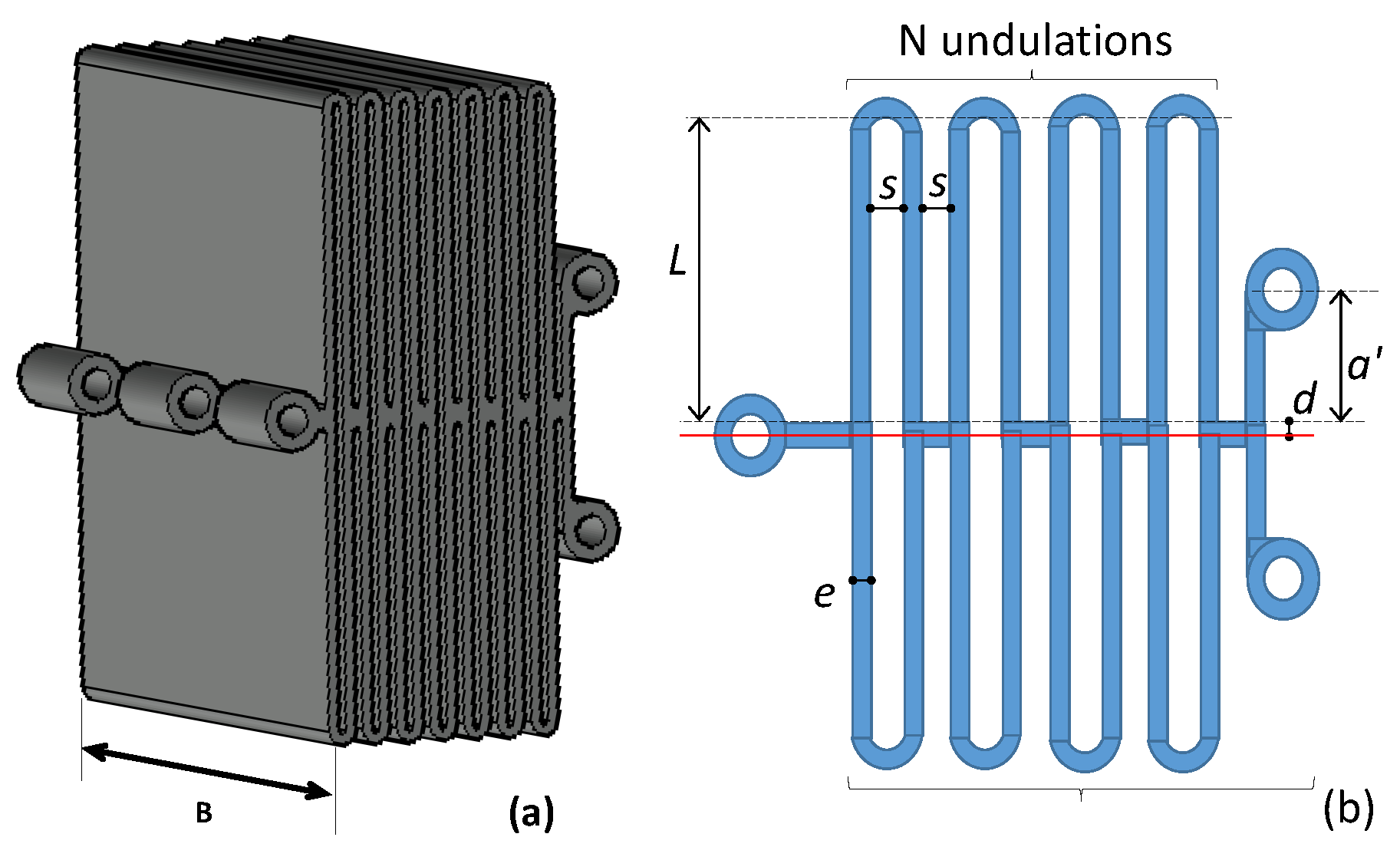
The equations of the resistance of materials were used to define the analytical model of the springs, considering the deformation capacity (45 mm) (Table 1) and load capacity (10,000 g) of the testing machine designed for these effects. Figure 3a and Figure 3b, respectively, show the 3D model and flat diagram of the type of spring built and used in the tests. Figure 4 presents the conceptual model for the analysis of the indicated spring, which considers its symmetry and allows the equations that relate the applied force F to the elongation u that it generates. These equations allow sizing the springs to ensure their behaviors in the linear elastic range when the dissipation device is deformed to its full capacity. Each spring was dimensioned using Equations (11)–(21), considering that the stiffest spring subjected to a force of 5000 g—50% of the capacity of the testing machine—reaches 75% of the elastic limit deformation of the PLA material, ε_el, at its most requested point.

To define the analytical model that allows the calculation of the stiffness of the spring, it was divided into two equivalent halves based on their symmetry. Each half of the spring, located on each side of the plane of symmetry, is made up of 2 types of elastic elements with stiffnesses, K₁ and K₂ (Figure 4a). In each half of the spring, there are 2N elements with the stiffness K₁ and 1 element with the stiffness K₂ (Figure 3b), all of them working in series. The second half of the spring works in parallel with its symmetrical counterpart, which allows associating a simplified analytical model to calculate its stiffness.

The stiffnesses K₁ and K₂ of the model, shown in Figure 4a, are given by:

$$K_1=\frac{12EI}{L^3}$$

(11)

$$K_2=\frac{3EI}{{a^{\prime }}^3}$$

(12)

$$I=\frac{1}{12}B{e}^3$$

(13)

Considering that in each symmetrical half of the spring, there are 2N elements with the stiffness K₁ and 1 element with the stiffness K₂ working in series, the equivalent stiffness of this set is given by:

$$K_{eq}^{\left(1/2\right)}={\left(\frac{2N}{K_1}+\frac{1}{K_2}\right)}^{-1}$$

(14)

Then, adding the contributions of both symmetrical halves of the spring working in parallel to each other, the theoretical stiffness of the complete spring is obtained as:

$$K_{eq}^{\left(T\right)}=2K_{eq}^{\left(1/2\right)}$$

(15)

To determine the modulus of elasticity E of the PLA material, necessary for determining the spring stiffness, the experimentally obtained equivalent stiffness of the spring, $K_{eq}^{\left(E\right)}$, was used. That stiffness was considered as the linear range stiffness obtained from the test of a sacrificial spring. Considering the above, the modulus of elasticity is defined by the following expression:

$$E=\frac{1}{12I}{K}_{eq}^{\left(E\right)}\left(N{L}^3+2a^3\right)$$

(16)

This modulus of elasticity is typical of the PLA material, which is why it was used for the design of all the other springs. The indicated springs must be designed with specific stiffnesses, also having the necessary deformation capacity to resist the maximum displacement level imposed in the tests.

Considering the analysis model of Figure 4a, the maximum stress in each of the constituent elements with the stiffness K₁, due to a force of F_E elongating the spring (Figure 4a), is given by:

$${\sigma }_1^{max}=\frac{F_{E}Le}{8I}$$

(17)

Similarly, the maximum stress in the constituent elements with the stiffness K₂ is given by:

$${\sigma }_2^{max}=\frac{F_E{a}_e^{\prime }}{4I}$$

(18)

The maximum displacement of the spring is limited by the size of the dissipating device. The geometric design of this dissipating device admits a maximum deformation, u_max = 45 mm, which generates a maximum extension in the spring of u_e^max = 30 mm (Table 1), consistent with Equations (1)–(6). Considering the above, the theoretical maximum force acting on the elastic element or spring was determined as:

$$F_{max}^{\left(T\right)}=K_{eq}^{\left(T\right)}·u_e^{max},$$

(19)

where $K_{eq}^{\left(T\right)}$ is the theoretical spring stiffness defined by Equation (15), combined with Equations (11)–(14), using the modulus of elasticity determined from the experimental results replaced in Equation (16).

Equation (19), replaced in Equations (17) and (18), allows for determining the maximum working stresses in the constituent elements of the spring. The maximum value of the indicated normal stresses defines the maximum stress and deformation of the spring material, according to Equations (20) and (21):

$${\sigma }_{max}=max\left({\sigma }_1^{max}, {\sigma }_2^{max}\right)$$

(20)

$${\epsilon }_{max}=\frac{1}{E}{\sigma }_{max}.$$

(21)

The maximum deformation of the elastic limit of the PLA material, ε_el, is determined with Equation (21), using the stresses σ₁^max and σ₂^max calculated according to Equations (17) and (18), replaced in Equation (20). In the calculation of the indicated stresses, the force F_E is determined in the test of the sacrificial spring brought to failure at the limit point of linear elastic behavior.

2.4. Preliminary Sizing of Springs

In addition to the constraints of spring stiffness and internal resistance to deformation of the PLA material, other geometric constraints were established. These are mainly due to the pre-established dimensions of the geometric design of the complete dissipation device (Table 1) and limitations due to the capacity of the 3D printer used. These restrictions on the sizing of the spring are the following: a = 11.5 mm; B = 60 mm; d = 1 mm (Figure 3a,b). The values assigned to these variables were considered constant for all springs, regardless of their stiffness.

Considering the above, the geometric design of the spring is summarized in the determination of the parameters: L, e, s and N (Figure 3b). Due to the predetermined size of the energy dissipator (Table 1), the length L should not be greater than 35 mm to allow the spring to fit inside the device. To ensure a good 3D printing resolution of the spring, the thickness e should not be less than 0.8 mm. Furthermore, in order to avoid leading to the very high rigidity of the spring or excessive use of material, the indicated thickness should be at most 2 mm. The separation s between the printed stripes (Figure 3b) should not be less than 0.5 mm to prevent adhesion between portions that must be printed without contact. Finally, the number of undulations N (Figure 3b) is determined in order to give the spring the necessary stiffness, imposing a restriction that 5 ≤ N ≤ 8 to delimit the amount of PLA used in its preparation in a 3D printer.

The geometry of each spring was designed to obtain the desired stiffness, ensuring that the maximum stress and deformation given by Equations (20) and (21) do not exceed 75% of the maximum deformation of the linear range of the PLA material when subjected to an elongation $u_e^{max}$ = 30 mm.

Each spring was designed so that it could withstand large elongations and only tension forces, in addition to being built in a 3D printer in PLA material. The “accordion” shape shown in Figure 3 was established as a feasible design since it facilitates support on the hotbed of the 3D printer, turning out to be very flexible and resistant. This element corresponds to the elastic part of the device that helps it return to its original shape once the external load has been removed. For this to be true, the PLA material must not exceed the elastic-linear working range.

2.5. Specific Model of the Dissipation Device

A physical prototype of the proposed device was built, according to the conceptual model of Figure 2a,b, with the overall dimensions shown in Table 1. This prototype was completely built on a 3D printer using PLA as material (Figure 5a,b).

The specific prototype of the dissipation device was made up of a set of parts that allow it to function according to the conceptual model presented above. The parts that make up the dissipation device are shown in Figure 6 and are given in the following: (1) casing with pins, (2) clamps with hooks, (3) connecting rods, (4) interconnection system, (5) transmission shaft with friction heads, (6) elastic element or spring, and (7) mobile clamping. The friction heads of element (5) are interchangeable. They serve two purposes: to distribute the load passed from the transmission shaft to the clamps in a finite area and not at a point and to modify the coefficient of friction between the shaft and the clamps by incorporating sheets of sandpaper on the surface of the ring-shaped heads.

2.6. Description of the Experimental Tests

Three types of tests were carried out: direct shear test to determine the coefficient of friction between sliding parts, traction test to calculate the stiffness of the elastic element, and load-unload cyclical test to determine the response of the dissipation device as a whole.

2.6.1. Direct Shear Friction Tests

An experimental test was designed to determine the coefficient of dynamic friction between two surfaces through the balance of the forces present. Dynamic friction is the one that acts between two surfaces when there is sliding between the parts in contact, and it is the one that generates the dissipation of energy. An experimental protocol was defined, and the test framework was built in a 3D printer using PLA material. The measurement system consists of three parts (Figure 7a), which are:

• Sliding Cart ①: It can slide on a rail aided by lateral bearings that direct the movement. Different masses can be added to it to increase the normal contact force between sliding surfaces. Two “tablets” attached to its lower part allow changing the materiality of one of the sliding surfaces.
• Guide Rail ②: It corresponds to a flat surface rail made of PLA, allowing a 30 cm run of the Sliding Cart on it. At its furthest end from the Sliding Cart, it has a pulley that allows the direction of the weight load as a lateral load on the Cart.
• Weight ③: A container filled with sand was used as a weight. This allows, by means of a cable and a pulley, to apply a lateral load to the Sliding Cart until the friction force is overcome.

Figure 7. Direct shear test. (a) Photograph of the test with its parts, (b) Schematic diagram with measurement variables.

Figure 7. Direct shear test. (a) Photograph of the test with its parts, (b) Schematic diagram with measurement variables.

As can be seen in Figure 8b, the blue pieces correspond to the PLA surface, while those in black correspond to the same PLA pieces, but with their surface covered with a sheet of sandpaper that allows increasing the coefficient of friction. These pieces are inserted into the perforated slots shown in Figure 8a under the sliding cart and fixed with the wooden dowels in Figure 8b.

The dynamic equilibrium of the sliding cart with added mass (total mass M) was formulated based on the diagram in Figure 7b once the dynamic friction had been overcome. In this condition, the force P is applied laterally to the car by the pulley, and the weight hanging from it is greater than the dynamic friction force F_R. In this way, the car has a constant net force P-F_R, and therefore, its acceleration ü is constant. The Coulomb’s friction was considered [39,40] so that the friction force is proportional to the normal force, according to Equation (22).

$$F_R={\mu }_{c}Mg$$

(22)

Considering the above, the variables involved in the test in Figure 7b are related by means of Equation (23):

$$M\ddot{u}=P-{\mu }_{c}Mg$$

(23)

The acceleration of the cart can be determined by means of the kinematics equations, considering that the net force is constant, based on the distance traveled, Δu, and the time to travel it, Δt, according to Equation (24).

$$\ddot{u}=\frac{2\Delta u}{\Delta t^2}$$

(24)

By combining Equations (23) and (24), the friction coefficient can be determined based on the variables measured in the test, according to Equation (25).

$${\mu }_c=\frac{P\Delta t^2-2M\Delta u}{Mg\Delta t^2}$$

(25)

For each pair of friction surfaces used (PLA-PLA and PLA-Sandpaper), two tests were carried out with different added masses on the sliding cart. Each test with a different mass was repeated three times to ensure the reliability of the results. The data acquired in these tests were the sliding time Δt elapsed to achieve a sliding Δu = 23 cm, in addition to the minimum hanging load P, necessary to overcome the static friction and start the cart moving. The tests were recorded on video from before the cart started its movement at u = 0 cm until it reached its final position considered at u = 23 cm. From the slow motion analysis of each video, it was possible to determine, with the precision of one-hundredth of a second, the time increment Δt that the cart took moving between the two positions indicated above in each test. A bucket, whose level of sand was gradually increased, was used until the static friction was overcome. The load P of each test corresponds to the weight of the bucket and the added sand up to the moment of incipient sliding of the cart.

2.6.2. Tensile-Elongation Tests of the Springs

These tests were used to measure the resistance to deformation and tension in the linear elastic range capable of resisting the PLA material, of which the spring of the device was made. In addition, it was used to experimentally determine the stiffness of the springs that would later be used in the tests of the device.

Five springs were built in a 3D printer. The N° 5, called a sacrificial spring, was subjected to a load-unload test in tension, bringing it to the breaking condition, exceeding the elastic range. This allowed us to determine the resistance to tension and deformation of the linear elastic limits of the PLA material, σ_el and ε_el. These were determined using Equations (20) and (21), substituting in them the force F_e^(el), corresponding to the highest force for which the force-elongation curve of the sacrificial spring maintains a linear relationship between the variables. These results—σ_el and ε_el—were incorporated into an analytical calculation model of the spring used in the tests to determine the maximum deformation and load that can be applied to each spring while maintaining its linear elastic behavior. This allowed defining the limits of deformation imposed in the experimental protocols of cyclical loading-unloading implemented to each one of the springs. The results of the tests allowed determining experimentally the rigidity in the linear elastic range of each of the springs built in a 3D printer with PLA material, which was later used in the tests of the dissipation device as a whole.

2.7. Tensile-Elongation Testing Machine

A device was designed and built in a 3D printer for the execution of the cyclic load-elongation test of the springs (Figure 9). This machine was used to carry out the cyclic tensile-elongation tests on the springs and on the complete dissipation device. Subsequently, a select group of tests of the dissipation device was repeated in a machine with more professional characteristics. This second machine is made of steel, and it is driven by a stepper motor controlled by a computer through Arduino UNO. The machine transforms the torque into linear force using a ball screw. In all cases, the test protocol contemplates the application of controlled deformation with a specific imposed displacement sequence.

2.7.1. Machine Built on a 3D Printer

For a detailed explanation of the testing machine, in this section, reference will be made to the components of the testing equipment according to the numbers indicated in Figure 9. Considering the pitch—or displacement in each complete turn—of the bolt used ③, each turn of the nut attached to the gear ① driven by a direct current motor with a speed reduction box ② imposes a displacement p = 1.41 mm/rev. on the spring ④—or tested device— fastened to a load frame ⑤ at its opposite end to the pin ③. The nut-gear system is in contact with a load cell ⑥ with a load measurement range of 10,000 g and a sensitivity of 1 g that is part of a digital kitchen scale ⑦ adapted to the equipment. An axial ball bearing was inserted between the load cell ⑥ and the gear nut ① to minimize the friction due to the rotation of the gear nut and thus achieve the least disturbed measurement possible. The gearbox motor ② has a rated speed of 600 rpm with a 24 VDC supply. However, a 6 VDC power source was used to further reduce the rotation speed, which is estimated at 150 rpm. The output shaft of the motor with reduction box ② is connected to the gear ① with a transmission ratio of 12/120, reducing the speed to 1/10, that is, approximately 15 rpm in the largest gear when having a 6 VDC power supply. Considering the above and a pitch p = 1.41 mm/rev. of the bolt ③, the estimated speed of application of the deformation is 0.35 mm/s. This is a conservative estimate since it would correspond to the deformation speed without resistance offered by the tested object and possible friction between the pieces of equipment. Therefore, this speed is reduced as the resistance of the tested object or specimen increases. Load measurements were recorded for the specifically imposed displacements corresponding to 1, 5, 10, 15, 20, 25 and 30 turns of the gear nut ①. These displacements correspond to the imposed elongations of 1.41, 7.05, 14.1, 21.15, 28.2, 35.25 and 42.3 mm, respectively. Because PLA is a thermoplastic material, the tests were carried out considering a 30-s pause after each short movement sequence that determines the points recorded in the load-displacement test to achieve load stabilization in each of them.

Figure 9. Assembly of a spring in the testing machine built on a 3D printer with PLA material.

Figure 9. Assembly of a spring in the testing machine built on a 3D printer with PLA material.

This test consisted of applying an imposed displacement u of cyclical nature at the mobile end of the device (Figure 1b). The displacement was applied in three loading and unloading sequences with increasing amplitudes. A single device casing was tested (Figure 10), but with two different coefficients of friction on the sliding surface under friction, permuted with two different elastic elements or springs of different stiffnesses (Figure 3b). The sliding ring-shaped heads were covered with sandpaper to modify the coefficient of friction between the sliding surfaces. These elements could be exchanged for an equivalent one with a PLA surface, leaving its counterpart with a PLA surface. In this way, it was possible to have sliding surfaces between the sandpaper and PLA and between PLA and PLA, thus having two different coefficients of friction, as previously determined. The stiffness of the elastic element was modified by exchanging it inside the device (element (6) in Figure 6), using two different springs previously built and tested to determine their corresponding stiffnesses.

This machine was used to carry out the tensile-elongation test on the N° 5 spring built in a 3D printer in PLA material (Figure 11). The indicated spring was tested until failure, which was assumed as the condition in which an increase in applied deformation generated a reduction in the measured force. In this failure condition, concentrated plasticity is evidently manifested at some points of the maximum stress in the material (Figure 11). Springs N° 1 to 4 were tested in the linear elastic range, and spring N° 5 was tested to failure in order to determine the resistance and deformation parameters of PLA in the elastic range. This allowed springs N° 1 to 4 to be geometrically designed to ensure their behavior in the linear elastic range for the deformation demand to which they would be subjected when inside the dissipation device.

2.7.2. Steel Testing Machine with the Electromechanical Actuator

A tensile testing machine built in metal and driven by displacement control using a stepper motor (Figure 12) was employed due to the load limitations that the machine built in a 3D printer has. The tests on the machine built on a 3D printer were carried out during the teleworking period due to the COVID-19 pandemic. In addition, when returning to face-to-face work, the University’s laboratory equipment and instruments were available. Therefore, to obtain more reliable results with a higher sampling rate, it was decided to repeat the tests of the complete dissipation device with this more professional equipment and instrumentation.

The test machine shown in Figure 12 has an electromechanical actuator controlled by displacement through an Arduino UNO board. The actuator is driven by a Longs Motor brand stepper motor, model NEMA 34HST9805-37b2, capable of exerting a sustained torque of 7 Nm with a controlled rotation of 1.8° per step. The motor is connected to a 16 mm diameter ball screw with a pitch p = 4 mm/rev., being able to describe the movement with a precision of 0.02 mm/step. Regarding the instrumentation, the force was measured with a GUANG CE brand S-type load cell, model YZC-516, with a capacity of 100 kg. The imposed deformation was measured using an LVDT-type displacement transducer with a maximum travel of 200 mm.

3. Results and Discussion

This section presents the results obtained from applying the methodology described in the previous section. These results are of three types, focused on the determination of (1) friction coefficient, (2) PLA resistance and spring stiffness, and (3) cyclical response of the device. This last type of test was carried out in two machines. The first was built with domestic materials—such as a motor with a gearbox for a baby car, a transformer to charge a cell phone, a kitchen weight for food, toothpicks, sandpaper for wood, multipurpose adhesive, among others—parts made in a 3D printer, and a direct current motor with gearbox, powered by a VAC220-VDC6 transformer. The second machine was built of steel and powered by a computer-controlled stepper motor.

3.1. Direct Shear Friction Tests

The data acquired in these tests were the sliding time Δt elapsed to achieve a sliding Δu = 23 cm, in addition to the minimum hanging load P, necessary to overcome the static friction and start the movement of the cart (Figure 7b). The experimental measurements indicated above are shown in Table 1 and

Table 2. Results of the critical slip experimental tests for PLA-PLA surfaces in contact.

Test N°	Mass of Cart, M (kg)	Hanging Weight, P (N)	Displacement Time, Δt (s)	Calculated Coefficient of Friction µc
1	1.67	5.51	0.69	0.237
2	1.67	5.72	0.68	0.249
3	1.67	5.10	0.73	0.224
4	3.67	10.42	0.75	0.207
5	3.67	10.81	1.12	0.263
6	3.67	10.64	0.77	0.217
			Average coefficient µm	0.233

. With these measurements and using Equation (25), the calculated friction coefficient μ_c of each test was determined, which is shown in the same tables. As mentioned in the methodology, each test was repeated three times. Therefore, six experiments were carried out for each different pair of surfaces in contact: three with a mass value of the sliding carriage and three with another value of the indicated mass. Then, using Equation (26), which uses the results of individual tests calculated with Equation (25), the mean friction coefficient of the indicated n = 6 tests was attained, obtaining a single friction coefficient for the PLA-PLA surface and one for PLA-Sandpaper.

$${\mu }_m=\frac{1}{n}{\displaystyle \sum }_{k=1}^n{\mu }_c^{\left(k\right)}$$

(26)

For each pair of friction surfaces used (PLA-PLA and PLA-Sandpaper), two tests were carried out with different added masses on the sliding carriage. Each test with a different mass was repeated three times to ensure the reliability of the results, which are shown in Table 2 and

Table 3. Results of the critical slip experimental tests for PLA-sandpaper surfaces in contact.

Test N°	Mass of Cart, M (kg)	Hanging Weight, P (N)	Displacement Time, Δt (s)	Calculated Coefficient of Friction µc
1	1.67	11.59	0.64	0.629
2	1.67	11.85	0.67	0.657
3	1.67	12.52	0.65	0.691
4	3.67	27.20	0.61	0.673
5	3.67	26.98	0.78	0.700
6	3.67	22.31	0.67	0.672
			Average coefficient µm	0.672

.

3.2. Geometric Spring Pattern

In order to determine the parameters of resistance to tension and deformation of the PLA material at the limit of its linear elastic behavior, one of the five springs was tested until it exceeded its yield point (see Figure 11 and Figure 13). For this test, the spring N° 5 of

Table 4. Geometric design parameters of the springs built on a 3D printer with PLA.

Spring N°	L (mm)	e (mm)	s (mm)	N
1	21.45	0.8	0.50	8
2	22.60	0.9	0.85	7
3	28.65	1.6	0.85	5
4	23.35	1.4	0.50	6
5	22.60	0.9	0.85	7

was used, which was designed assuming arbitrary values of the parameters L, e, s and N (Figure 3b), but complying with the restrictions mentioned above for the parameters a, B and d. This is because, a priori, the modulus of elasticity of the material and its resistance to deformation in the linear elastic range was not known, which is sought to be obtained with this test.

Figure 13 shows the results of the tensile-elongation test of the spring N° 5, where two curves corresponding to instantaneous load and stable loads can be observed. The first was built by applying discrete displacement increments and measuring the load just after the displacement was applied. The stable load curve was obtained considering the same displacements imposed but measuring the load registered after 30 s of applying the displacement. It can be seen in Figure 13 that the instantaneous load and the stable load are practically the same in the zone of linear elastic behaviors of the material, that is, up to approximately 40 N of applied force. Once the threshold is exceeded, the curves show noticeable differences, with force recorded in the stable load curve being lower than in the instantaneous load curve, the first reaching up to 50.6 N and the second up to 51.1 N. This is because PLA is a thermoplastic material and may show creep for near-failure load levels.

The results shown in Figure 13 determined the experimental stiffness and elastic limit load of the spring. The first was considered the slope of the stable load curve within the linear elastic range. The elastic limit load of the spring was considered equal to 40 N, which is where the beginning of the changes in the slopes of both curves or loss of linearity can be seen.

The modulus of elasticity of the PLA material calculated with Equation (16) for the sacrificial spring (N° 5), whose dimensions are indicated in Table 4, was E = 2183 N/mm². In the calculation of E, the stiffness obtained experimentally $K_{eq}^{\left(E\right)}$ = 1.19 N/mm was used, corresponding to the slope of the initial straight line of the stable load curve in Figure 13. Equations (20) and (21) allowed us to determine the elastic limit deformation —ε_el— of the PLA considering an elastic limit force F = 40 N, resulting in ε_el = 0.0131. With the results mentioned above, and considering Equations (11) to (21) and the previous geometric restrictions, the dimensions of springs 1 to 4 to be tested in the linear range were calculated (Table 4).

The geometric sizing of spring N° 5—sacrificial spring—does not obey resistance or stiffness calculations, and its dimensions were arbitrarily assigned in order to determine the mechanical properties of the PLA material. The dimensions of springs 1 to 4 were defined in order to obtain the stiffnesses in a wide range, considering the tensile capacity (10 kg) and imposed stretching capacity (45 mm) of the machine designed and built on a 3D printer to carry out the tests. It was considered that all the springs must resist stretching u_max = 30 mm without exceeding the admissible deformation equal to 75% of the elastic limit deformation, that is, ε_adm = 0.75ε_el, according to the previously described calculation methodology.

The maximum strain for verification of springs N° 1 to 4 was calculated with stresses ${\sigma }_1^{max}$ and ${\sigma }_2^{max}$ (see Equations (17) and (18)) determined using $F_{max}^{\left(T\right)}$ given by Equation (19), considering $K_{eq}^{\left(T\right)}$ from Equation (15), with E = 2183 N/mm² determined for PLA (

Table 5. Mechanical and resistance parameters of the springs built in a 3D printer with PLA.

Spring N°	${\mathit{K}}_{\mathit{e}\mathit{q}}^{\left(\mathit{T}\right)}$ (N/mm)	${\mathit{F}}_{\mathit{m}\mathit{a}\mathit{x}}^{\left(\mathit{T}\right)}$ (N)	${\mathit{\sigma }}_1^{\mathit{m}\mathit{a}\mathit{x}}$ (N/m2)	${\mathit{\sigma }}_2^{\mathit{m}\mathit{a}\mathit{x}}$ (N/m2)	εmax(1)
1	1.02	30.6	25.64	2749	0.0094
2	1.41	42.3	29.51	30.02	0.0103
3	5.36	160.9	44.99	36.12	0.0155
4	5.58	167.4	49.86	49.11	0.0171

⁽¹⁾ Calculated with Equation (21).

). The deformation thus obtained was contrasted with the admissible deformation ε_adm = 0.75ε_el = 0.0098.

3.3. Tensile-Elongation Tests of the Springs

Each of the springs, whose geometry is described in Table 4, was tested under loading and unloading until reaching a maximum displacement of 40 mm. This corresponds to the maximum demand of 30 mm, reached with the maximum deformation allowed by the dissipation device built in a 3D printer, divided by the reduction factor 0.75, or until reaching the maximum capacity of 10 kg of the testing machine built in a 3D printer. Figure 14 shows the results of the experimental stress-elongation tests for each spring designed, including spring N° 5, tested in the elastic range before loading it to failure. The results were separated by stable load and unload curves in order to identify the experimental slopes corresponding to the stiffness of each elastic element. Curves with steeper slopes correspond to the springs with greater stiffness.

In Figure 14, the stiffnesses of the loading and unloading curves were obtained as the slope of the best equation of the fitted line by minimizing the sum of the squares of the difference with respect to the experimentally measured data. In this figure, it can be seen that the charge and discharge curves of individual springs are slightly different. Therefore, the theoretical stiffness described by the analytical model given by Equation (15) only considers a spring with a single stiffness. This stiffness was considered as the average of the stiffnesses in load, $K_r^{\left(c\right)}$, and in unloading, $K_r^{\left(d\right)}$, given by Equation (27), in order to compare the analytical predictions of the stiffness of the individual spring with the experimental values obtained with the indicated equation, as shown in

Table 6. Experimental stiffnesses at load, at unload, average and theoretical of individual springs tested.

Spring N°	Stiffness under Load Kr(c) (N/mm)	Unloading Stiffness Kr(d) (N/mm)	Average Experimental Stiffness Kr (N/mm)	Analytical Stiffness Keq(T) (N/mm) (1)
1	0.82	0.84	0.83	1.02
2	1.13	1.19	1.16	1.41
3	4.69	4.82	4.75	5.36
4	4.93	5.16	5.05	5.58
5	1.11	1.18	1.15	1.41

⁽¹⁾ Calculated with Equation (15), using the spring dimensions from Table 4 and the modulus of elasticity E = 2183 MPa for the PLA.

.

$$K_r=\frac{1}{2}(K_r^{\left(c\right)}+K_r^{(d)})$$

(27)

3.4. Cyclic Load-Unload Tests on the Device

3.4.1. Tests Made on a Machine Built in a 3D Printer

Table 7. Parameters of the forcing and the device in the execution of the cyclic load tests in a machine built on a 3D printer.

Test N°	Width of Cycles, umax (mm)	Average Coefficient of Friction, µm	Spring Stiffness, Kr (N/mm)
1A	6/20/34	0.233	1.16
2A	6/20/27	0.233	5.05
3A	6/20/34	0.672	1.16
4A	6/20/27	0.672	5.05

shows the results of the tests carried out with the assembly shown in Figure 10. A total of four devices with different characteristics of the coefficient of friction and stiffness of the elastic element were tested. This is because the indicated assembly has certain limitations, one of them being that it can only measure a maximum tension of 10 kg. In addition, the tension marked by the kitchen weight of the testing machine built on a 3D printer for the indicated assembly must be recorded on video. The forces for each discrete displacement imposed in the deformation cycles must be extracted from the video. Given these conditions, the device with a spring with a stiffness of K_r = 5.05 N/mm was only essayed up to a maximum of 27 mm of deformation.

Figure 15 shows the experimental results of the four tests carried out on the device in the machine built on a 3D printer. In the figure, each column of graphs represents the device with the same spring but with a different coefficient of friction µ, being µ constant in each row of graphs. It can be seen that when the force registered in the device increases, the stiffness K_r of the elastic element inside it becomes higher. It can also be observed that when increasing the friction coefficient, there is also an increase in the force, but the increase is less than when increasing the stiffness. Furthermore, the higher the coefficient of friction, the higher the energy dissipated by the device at the same spring stiffness. The dissipated energy also increases with the increasing spring stiffness, keeping the coefficient of friction constant. Consequently, the force with which the device responds and the energy dissipated in a complete load-unload cycle depends on the rigidity of the elastic element and on the coefficient of friction. The dissipated energy increases exponentially, and this causes the displacement imposed on the device in the load-unload cycle to become greater.

3.4.2. Tests Made on a Machine with the Electromechanical Actuator

With the experimental setup presented in Figure 12, a single casing of the device was tested, but with four different springs and two different coefficients of friction, which resulted in eight different tests, whose parameters are presented in

Table 8. Parameters of the forcing device and the execution of the cyclical load tests in a machine with an electromechanical actuator, commercial load and displacement sensors.

Test N°	Cycle Deformation Amplitude, umax (mm)	Average Coefficient of Friction, µm	Spring Stiffness, Kr (N/mm)
1B	34	0.233	0.83
2B	34	0.233	1.16
3B	34	0.233	4.75
4B	34	0.233	5.05
5B	34	0.672	0.83
6B	34	0.672	1.16
7B	34	0.672	4.75
8B	34	0.672	5.05

. The stiffnesses of the springs and coefficients of friction were obtained in the same manner as for the tests of the device in a machine built into a 3D printer, according to the methodology in Section 2.6 and the results in Section 3.1, Section 3.2 and Section 3.3. The movement sequence imposed by the actuator was ten cycles of loading and unloading of the sawtooth type, with an amplitude of 34 mm and a deformation speed of 12 mm/s.

Figure 16 shows the results of the experimental tests carried out with the experimental setup and instrumentation presented in Figure 12. In each graph, the tests with the same coefficient of friction are presented but with different spring stiffnesses. From the results obtained, the greater the stiffness of the elastic element or spring, the greater the force provided by the device. This is visibly noticeable since each graph presents curves with different inclinations according to the stiffness of the spring. It can also be seen that the greater the coefficient of friction, the greater the force the device provides in the loading branch. Regarding the energy dissipated in a load-unload cycle, the energy dissipated is proportional to the friction coefficient, and if this is increased, the energy dissipated by the device in a complete cycle is greater. Furthermore, it can be seen that the dissipated energy is also related to the stiffness of the elastic element inside the device, and if there is a greater rigidity, the greater energy will be dissipated by the device. The foregoing is consistent with what was observed in the results of the tests carried out on the machine built on a 3D printer in the previous section.

3.5. Comparison of the Analytical and Experimental Results

The experimental results of the cyclic load-unload tests on the device, shown in Section 3.4, were compared with the numerical predictions. For the above, the analytical model of the device defined by Equation (10) was used, with the coefficients of friction and stiffnesses of springs determined experimentally in Section 3.1 and Section 3.3, respectively. The experimental results in Section 3.1 and Section 3.3 are independent of the results of the cyclic load-unload tests of the device shown in Section 3.4. These tests—Section 3.1 and Section 3.3 versus Section 3.4—are double-blind and, therefore, allow the analytical formulation of the device to be validated with its experimental results. The comparison of the experimental results and analytical predictions are only shown for load-unload cycles of greater amplitude in each of the tests carried out.

The experimental results from Section 3.4 are shown in Figure 17, superimposed with the respective analytical predictions, calculated as above. In the figure, the area enclosed by each curve corresponds to the energy dissipated by the device in the load-unload cycle. It can be seen that these areas, although they are not the same between the experimental and analytical results, are similar and follow the same trend. That is, the greater the stiffness of the spring, the greater the force with which the device responds, as well as the greater the energy dissipation in one cycle. Furthermore, the dissipated energy increases when the coefficient of friction between the sliding surfaces increases. Also, the greatest differences between the analytical model and the experimental tests occur for the highest coefficient of friction. These differences are attributed to the fact that the analytical model overestimates the dissipation capacity of the device for larger friction coefficients and underestimates it for lower friction coefficients. This may be due to the fact that the roughness of the surface covered with sandpaper is very high, and there is a mechanical bond that leads to Coulomb friction—friction force proportional to the product between the friction coefficient and normal force—is not a good approximation in this case. Due to the above, Equation (26)—which uses individual test results calculated with Equation (25)—may not be a good estimator of the effective coefficient of friction between surfaces. Another possible explanation for the differences between the analytical predictions and experimental results is that the items used in the test in Section 3.1 are not flat, smooth surfaces. Instead, these elements have perforations to allow the fastening of the interchangeable frictional elements (Figure 8b). These holes could have ridges that could generate mechanical binding that would lead to an overestimation of the coefficient of friction. This would lead to analytical results that would overestimate the energy dissipation capacity by using a friction coefficient higher than that corresponding to the sliding surfaces of the device tested in Section 3.4, where the surfaces are flat.

The shapes of the load-displacement curves and the dissipated energy—area enclosed between the charge-discharge curves—are similar between the experimental tests and the analytical predictions of the device. The greatest difference between the two groups of curves is observed between the discharge branches, this difference being more noticeable at the beginning of the discharge. This can be attributed to the friction between the pieces of the device, which are slightly different from those that the analytical model considers. The physical device included “rings-shape heads” installed on the load transmission cylindrical shaft that interact with the clamps (Figure 6b). However, in the analytical model, the load transfer occurs directly between the cylindrical axis and the clamps (elements (5) and (3) in Figure 1a).

From the experimental results and analytical predictions shown in Figure 17, the energy dissipated in each of the tests was determined. It corresponds to the area enclosed between the charge and discharge curves and was determined using the command trapz(X, Y) in the Matlab software. This command performs a numerical integration using Simpson’s rule, which evaluates the area between two discrete points, considering a straight line between them.

Table 9. Dissipated energy values were calculated with the experimental results and the analytical models.

Test N°	Average Coefficient of Friction, µm	Maximum Amplitude, umax (mm)	Experimental Energy (J)	Theoretical Energy (J)	Relative Error (%)
1	0.233	34	0.126	0.108	16.6
2	0.233	34	0.141	0.129	9.3
3	0.233	34	0.521	0.501	4
4	0.233	34	0.589	0.551	6.9
5	0.672	34	0.178	0.229	22.3
6	0.672	34	0.255	0.316	19.3
7	0.672	34	0.707	1.289	45.15
8	0.672	34	0.869	1.352	35.72

shows the calculated results of the energy dissipated by the device in each experimental test, as well as its equivalent analytical prediction, indicating the maximum displacement amplitude with which they were obtained. With the data shown in the table, it can be confirmed that in the experimental tests with sliding between PLA–PLA, the device behaves more similarly to the analytical prediction than in the case of sliding between PLA-Sandpaper. Table 9 also shows the relative error, ${\epsilon }_{ϵ}$, between the dissipated energy determined experimentally, ${ϵ}_{exp}$, and the corresponding one calculated analytically, ${ϵ}_{an}$, defined as:

$${\epsilon }_{ϵ}=\frac{\left|{ϵ}_{an}-{ϵ}_{exp}\right|}{{ϵ}_{an}}100\%$$

(28)

It must be taken into account that the experimental results shown in Figure 17 and Table 9 were made in a model built in PLA material in a 3D printer. In other words, it is not a prototype for use in real structures. In continuation of this line of research, the authors of this paper are working on designing and constructing a functional prototype for use in the seismic protection of industrial storage racks. The preliminary experimental results of the prototype have a much better fit with the numerical model. These results allow us to infer that the relatively large errors observed in Table 9 are not attributed to the analysis model but to the characteristics and materiality of the prototype built on a 3D printer. Despite the above, the results below mark a clear trend and indicate that, in general terms, the proposed device behaves as the analysis model predicts.

Table 9 shows all the tests carried out, but Figure 17 only shows half of them. This is because, with the figure, we only wanted to show the tendency that the curves show when changing the stiffness and the coefficient of friction.

3.6. Device Differentiation with the Existing Technologies

This section shows a comparison of attributes of a group of 7 energy dissipation devices, considering the one proposed here, for their use in the seismic protection of structures. Each device has been cataloged with a code from D0 to D6 to cite in

Table 10. Comparison of the attributes of the proposed device with those described in the literature.

Attributes (1)	Devices
	D0 (2)	D1	D2	D3	D4	D5	D6
Bibliographic reference		[12,13,24]	[15,16,17,28]	[20,21,27]	[22,23,25]	[26,32,33]	[34]
Wich is the way of dissipation? (FV, VE, FM, F) (3)	F	FM	VE	FV	F	F	FM
self-centering capability? (1)	1	0	0	0	0	1	1
Usable in prestressed cables? (4)	1	0	0	0	0	0	1
Requires activation force? (4)	1	0	1	1	0	1	1
Energy dissipated increases quadratic to displacement? (4)	1	1	0	0	0	1	1
Fatigue is local or global? (4*)	1	0	1	1	1	1	1
Maintenance requires qualified personnel? (4)	1	1	0	0	1	1	1
Manufacturing in metalworking industry? (4)	1	1	0	0	1	1	NC (5)
Total	7	3	2	2	3	6	6

⁽¹⁾ It is called “1” when the attribute is favorable and “0” when it is unfavorable, in order to add the points per device. ⁽²⁾ Device proposed in this investigation. ⁽³⁾ FV: Viscous fluid flow, VE: Viscoelastic, FM: Metal creep, F: Frictional. ⁽⁴⁾ Yes: 1, No: 0; ^(4*) Local: 1, Global: 0. ⁽⁵⁾ Not conclusive.

, which shows the summary of the comparison made. Each device is described below in terms of its operation, attributes and bibliographical reference.

D1: Most common Metal Creep Devices such as the TADAS, described by Tsai et al. [12], the honeycomb damper proposed by Kobori et al. [13], and the one proposed by BehkamRad et al. [24]. These heatsinks lack an autonomous self-centering system. They work in one direction but not in both directions. They require a minimal activation force—yield force—to achieve energy dissipation. After a severe earthquake, they must be inspected to verify that there is no material fatigue or severe damage. If the above is detected, the device must be completely changed. This device can be manufactured by a metalworking company.

D2: Devices that dissipate by deformation of a viscoelastic material. Some of them are the ones proposed by Wang et al. [15], Chang et al. [16], Lai et al. [17] and Aiken [28]. They are characterized by their dependence on the strain rate. They lack a self-centering system, but they do not oppose resistance to the structure so that they return to their original position. They can work in both load directions and do not require a minimum activation force. However, they must be inspected to verify that there is no loss of viscoelastic material or severe damage after an earthquake. If damage is determined, they must be changed by the companies in charge of the manufacture.

D3: Devices that dissipate by the flow of a viscous fluid. They are those of Lee et al. [20], Sorace et al. [21], and Li et al. [27]. They are characterized by depending on the speed of excitation to dissipate energy. They lack self-centering, but they do not oppose resistance to the structure so that they return to their original position. They can work in compression or traction equally. They must be inspected to verify that there is no loss of fluid after a severe earthquake. If damage is detected, it must be changed by the companies in charge of the manufacture.

D4: Devices that dissipate by the frictions between two or more surfaces. Some of them are those of Dai et al. [22] and Lee et al. [23,25]. They are characterized by not depending on the excitation speed to dissipate energy but on the displacement. They lack self-centering and can resist the structure so that they return to their original position. They can work in both load directions and require a minimum activation force. After a severe earthquake, they must be verified that there is no excessive wear of the materials. If there is some wear, the contact surface can be changed, which is easily manufactured by metal-mechanic companies.

D5: Devices that dissipate via the frictions between two or more surfaces and add a component that allows self-centering. Some of them are those of Wang et al. [26], Veismoradi et al. [32] and Westenenk [33]. They are characterized by not depending on the excitation speed to dissipate energy but only on the displacement. They can work in both load directions and require a minimum activation force. After a severe earthquake, it must be verified that there is no excessive wear of the materials. If there is some wear, the contact surface can be changed, which is easily manufactured by metal-mechanic companies.

D6: Device that dissipates by deforming a metal with shape memory, which gives it the ability to self-center. It was proposed by Gao et al. [34] and can be implemented with cross-bracing cables. The damper dissipates proportionally to the deformation and does not require an activation force for its operation. After a severe earthquake, the fatigue of the material must be verified, and, in such a case, the metal ring must be changed carefully.

As shown in Table 10, the device proposed here differs from a state-of-the-art device in several aspects. It has comparative advantages with respect to the existing technologies, and the idea of a dissipator has the potential to be implemented in seismic protection and rehabilitation of structures.

3.7. Discussion, Attributes and Application of the Proposed Dissipator

An energy dissipation device by friction that works in tension and has a self-centering capacity, whose design is original by the authors, is presented in this investigation. The device was thought to be used in structures to control vibrations produced by dynamic loads such as earthquakes.

It must be noted that the experimental results presented in this paper correspond to a prototype built in PLA material in a 3D printer. Therefore, it does not have the resistance nor the dissipation capacity to be used in real structures. The objective of the experimental tests presented here points to two aspects. The first is to verify that the device has the attributes expected of it based on its conceptual model, that is, to verify the proof of concept. The second is to verify that the simplified analytical model of the device reproduces its experimental behavior with relative fidelity.

The expected attributes of the device are (1) self-centering capability and (2) energy dissipation capability that increases in approximately quadratic proportion with strain demand. The first attribute was satisfactorily fulfilled since the tested device was able to recover its original shape without permanent deformations (Figure 15 and Figure 16). It was also possible to verify the second attribute, which is not so evident, but it can be demonstrated by analyzing the information of the legends in Figure 15, which are summarized in

Table 11. Energy dissipation capacity of the device was tested on a machine built on a 3D printer for different amplitudes of the imposed deformation, friction coefficient and spring stiffness.

Test N°	Amplitude umax (mm)	Av. coeff. of Friction µm	Spring Stiffness, Kr (N/mm)	Energy Dissipated, ED (mJ)
1A	6	0.233	1.16	7
	20	0.233	1.16	79
	34	0.233	1.16	184
2A	6	0.233	5.05	24
	20	0.233	5.05	177
	27	0.233	5.05	276
3A	6	0.672	1.16	17
	20	0.672	1.16	116
	34	0.672	1.16	271
4A	6	0.672	5.05	31
	20	0.672	5.05	257
	27	0.672	5.05	416

and Figure 18.

Figure 18 clarifies that the energy dissipation capacity of the device follows a non-linear relationship with the displacement amplitude in the load-unload cycle. This relationship approaches a quadratic behavior. It is also noted that the dissipated energy can be increased in the device by increasing the coefficient of friction and by increasing the stiffness of the spring within the device. The coefficient of friction between two surfaces assumes physically bounded values, so the increase in dissipation capacity that can be achieved by increasing it is limited. However, the stiffness of the spring can be as great as desired, depending on the application for which the device is used. Therefore, the attributes of the proposed device are easily scalable in resistance and energy dissipation capacity by increasing the stiffness of the spring inside. This makes the proposed device versatile and can be implemented in various applications.

Because the device works only in tension, to be effective in protecting structures subjected to cyclical vibrations, it must be pre-tensioned. Considering the above, it can be implemented in post-tensioned diagonal bracing of structural frames, such as in bracing towers of industrial storage racks of the selective type (Figure 19). In this case, it is required that in the same span, there are two post-tensioned diagonals bracing, each with an energy dissipation device. The arrangement can be similar to the one presented by Sorace et al. [25] for his energy dissipation device (Figure 20a). This has the advantage that it makes it possible to take advantage of the attributes of the device mentioned above, in addition to increasing the energy dissipation capacity for small deformations. In Figure 20b, the characteristic hysteresis curve for the arrangement of Figure 20a is shown, calculated with the analytical model of Section 2.2, considering the contributions of the two devices.

As seen in Figure 20b, a potentiated effect is achieved by including in flexible frames the combined action of two prestressed devices such as the one proposed here. The result is a macro-device that dissipates a greater amount of energy, even for low levels of imposed deformation. It has a self-centering capacity and provides additional rigidity to the structural system. The last two attributes allow for reducing residual story drifts, having the potential to enhance the overall structural resilience [37].

The authors are beginning to research the design and construction of a functional prototype made of steel for use in the seismic protection of industrial storage racks. The preliminary experimental results of the prototype have a much better fit with the numerical model than here. These results allow us to infer that the relatively large errors observed in Table 9 are not attributed to the analysis model but to the characteristics and materiality of the prototype built in a 3D printer. Despite the above, the results presented mark a clear trend and indicate that, in general terms, the proposed device behaves as the analysis model predicts.

4. Conclusions

In this investigation, a novel device for dissipating energy by friction with self-centering capacity, originally designed by the co-authors of this article for its use in the control of vibrations in structures, was presented. A conceptual model of the device was presented, which describes its fundamental components. An analytical model for the mechanical characterization of the device was formulated, based on the mechanical equilibrium of it and its components, considering the interaction between them in a deformed condition with large displacements.

A modular prototype of the proposed device was designed and built in a 3D printer with PLA material. This device allows the exchange of the frictional element and the elastic element inside it. This makes it possible to modify the coefficient of friction between the sliding parts and the rigidity of the elastic component of the device, being able to obtain different versions of the device. A theoretical design of the elastic element constituting the device was carried out, which was validated by means of experimental stress-elongation tests that allowed for determining its effective rigidity. The friction coefficients between two pairs of sliding surfaces, PLA-PLA and PLA-Lija, were also experimentally determined. This allowed the assembly of eight dissipation devices with different characteristics, which were subsequently tested and experimentally subjected to charge-discharge cycles with different displacement amplitudes. The experimental results were contrasted with the analytical predictions that used the results of stiffnesses and friction coefficients previously determined. The foregoing is in order to perform a validation of the double-blind analytical model.

Based on the results above, it was possible to determine that the device behaves experimentally in the way the analytical model predicts it, being capable of self-centering and dissipating energy proportionally to the imposed displacement. The behavior trends of the device response in terms of force and energy dissipated in a charge-discharge cycle are consistent between the experimental results and the analytical predictions. It was determined that the greater the rigidity of the elastic element, the greater the force with which the device responds and the greater its energy dissipation capacity. This dissipation capacity is also amplified by increasing the coefficient of friction between the sliding surfaces subjected to friction. It was possible to verify that the energy dissipated in a charge-discharge cycle increases significantly as the maximum imposed displacement increases. This is because a greater displacement leads to a greater force reaction by the device, which also increases the normal force between the sliding surfaces subjected to friction. This, in conjunction with the increase in slip with the increase in imposed displacement, causes the dissipated energy to increase approximately in a quadratic proportion to the imposed displacement amplitude.

In general, the design of the proposed device meets the energy dissipation expectations predicted in the conceptual model, the experimental results being consistent with the analytical predictions. The device showed great potential for structural applications and vibration control of mechanical systems.

5. Patents

The technology presented in this research has intellectual property protection through patent application N° PCT/IB2022/057524, dated 12 August 2022, and filed at the WIPO International Office, by the UNIVERSIDAD CATÓLICA DE LA SANTÍSIMA CONCEPCIÓN, with the title: ENERGY DISSIPATER FOR TRACTION LOADS.