Development of a Low-Cost Luminance Imaging Device with Minimal Equipment Calibration Procedures for Absolute and Relative Luminance

Abstract

Luminance maps are information-dense measurements that can be used to directly evaluate and derive a number of important lighting measures, and improve lighting design and practices. However, cost barriers have limited the uptake of luminance imaging devices. This study presents a low-cost custom luminance imaging device developed from a Raspberry Pi microcomputer and camera module; however, the work may be extended to other low-cost imaging devices. Two calibration procedures for absolute and relative luminance are presented, which require minimal equipment. To remove calibration equipment limitations, novel procedures were developed to characterize sensor linearity and vignetting, where the accurate characterization of sensor linearity allows the use of lower-cost and highly non-linear sensors. Overall, the resultant device has an average absolute luminance error of 6.4% and an average relative luminance error of 6.2%. The device has comparable accuracy and performance to other custom devices, which use higher-cost technologies and more expensive calibration equipment, and significantly reduces the cost barrier for luminance imaging and the better lighting it enables.

1. Introduction

Lighting design has historically been limited to illuminance measurement, in part due to technological limitations. However, new technologies, such as imaging photometers, also called luminance imaging devices, are now available, which can capture luminance maps. Luminance maps are analogous to images produced by conventional photography; however, instead, each pixel represents an accurate luminance measurement. Luminance maps better reflect human vision and, as such, can be used to better guide the application of lighting toward human vision and lead to significantly improved lighting efficiency and performance [1]. In particular, they can be used to directly evaluate important lighting measures such as discomfort glare (UGR) [2], which is typically evaluated indirectly and inaccurately, and also to evaluate promising alternative lighting measures such as Mean Room Surface Exitance (MRSE) [3,4]. Therefore, increasing the ubiquity of luminance imaging devices and increasing the incorporation of luminance maps and their derived measures into lighting practice will lead to improved lighting design. Additionally, luminance imaging devices are well served to meet the growing awareness and consideration of lighting quality [5,6,7].

Cost is a major barrier to the adoption of luminance imaging, with commercial options costing around USD 45,000 (LumiCam) [8,9]. However, low-cost electronics have enabled low-cost luminance imaging. Custom luminance imaging devices have been developed from a range of lower-cost imaging devices, including research CCD cameras [10,11,12,13,14], commercial digital cameras [15,16,17,18], 360° panoramic cameras [19,20], a Raspberry Pi (RPi) with a camera module [21], and High Dynamic Range (HDR) cameras [22]. Expensive CCD camera sensors have a more linear response to light, enabling easier calibration and greater accuracy [23]. However, commercial digital cameras often perform internal image processing to capture aesthetic images, increasing non-linearity, which complicates calibration for luminance measurement [15].

Three processes for calibrating digital cameras for luminance imaging are High Dynamic Range (HDR) imaging, Vignetting correction, and digital-to-luminance conversion. HDR imaging compiles images at multiple exposure speeds to increase the brightness measurement range [24], requiring manual or software image processing [16,17]. Vignetting is a characteristic dimming towards the image periphery [25] and must be characterized to obtain luminance measurements across the FOV. Finally, digital color readings (RGB) must be related to luminance by a standard equation [21] or a custom relationship [16].

These calibration methods require expensive, less common equipment, including integration spheres [10,12,21], uniform light-boxes [11,26], standard light sources [10,11,26,27], imaging photometers [13], luminance meters [11,13,15,21,22,28,29], and spectral response systems [21]. Further, device calibration and image acquisition with custom luminance cameras are involved and manually intensive [13,15,18,21]. The expensive calibration equipment presents a significant barrier to adopting luminance imaging [21]. Hence, custom devices are not a reasonable substitute for practitioners at this time.

This study presents new, low-cost methods and hardware. Low-cost luminance and relative luminance calibration procedures are presented, which enable the use of low-cost and highly non-linear sensors, and eliminate the need for uniform sources for vignetting and luminance calibration typically required. The luminance calibration procedure requires only a luminance meter and a steady light field, which can be produced with a variety of common lamp types. The relative luminance calibration procedure only requires a commonplace illuminance meter and a steady light field. The methods presented can be readily applied to smartphone technologies to make luminance imaging further accessible. Together, these methods overcome the need for expensive equipment and make useful luminance measurement far more accessible to lighting practitioners and thus more readily implemented and used to optimize lighting in practice.

2. Materials and Methods

The methods and materials section is laid out as follows: Section 2.1 introduces the main general steps for calibration for a custom imaging device; Section 2.2 discusses the required specifications for a successful device; Section 2.3 describes the selection, development, and specifications of the imaging device, and subsequently describes the methodology for each step of the device calibration process, following sequence of steps in Section 2.1; Section 2.4 details how, and against what standard, the performance of the resultant device is assessed.

2.1. Characterisation and Calibration Methods for Custom Imaging Devices

There are three different characterization and calibration procedures for custom luminance imaging devices: (1) sensor linearity; (2) vignetting; and (3) digital color reading to absolute and relative luminance calibration.

2.1.1. Sensor Linearity

Building environmental light covers several orders of magnitude. Achieving this range requires HDR imaging, and HDR imaging requires characterization of the pixel response. Pixel response is observed as the digital response to incident light, as illustrated by the example in Figure 1. For low-cost and highly non-linear sensors, or where the response has been manipulated by internal image processing, such as gamma compression [15], the pixel response must be accurately characterized with a non-linear model. In this work, pixel response is characterized by simulating increasing sensor illuminance with incrementally increasing exposure time, which has the same effect as increased illumination, yet requires less equipment.

2.1.2. Vignetting Characterisation

Vignetting is typically characterized by imaging a uniform field produced with expensive equipment, including integration spheres [10,12,15,18,21], uniform light boxes [11,26], or luminous ceilings [17]. An alternative procedure is presented, which requires only a steady non-uniform field, where dimming may be mapped by only changing the camera orientation. A target is imaged in the center of view and reimaged at some off-center position. As the target luminance is constant, the difference in target readings is due to vignetting at the off-center position and is the ratio of the two.

2.1.3. Color Readings to Luminance Calibration

Custom devices have been calibrated against luminance meters [11,15,16,17,18,22,29], standard light sources [10,12,15], and imaging photometers [13]. To minimize calibration equipment requirements, two low-equipment calibration procedures are developed: (1) an absolute luminance calibration requiring only a luminance meter and (2) a relative luminance calibration using only a common illuminance meter.

Luminance is calculated from camera color intensity readings. Where color measurements are assumed accurate, relative luminance (rL) can be found by definition of the RGB color space CIERGB (International Commission on Illumination), defined as follows [30,31]:

rL = 0.2126R + 0.7152G + 0.0722B

(1)

where R, G, and B are the measured color intensities in the RGB space. The resulting relative luminance may be scaled to absolute luminance measurements [15,16,21]. A similar approach is used in the SmartBeam Luminance Camera application; however, instead of scaling with a luminance reading, manufacture-reported sensor sensitivities are used to scale the results [32]. Internal settings, such as auto-white balancing (AWB) [33], lead to inaccurate color measurements and high luminance measurement errors, particularly for highly saturated colors [16]. Hence, these approaches have low accuracy.

In this work, absolute luminance calibration overcomes these inaccuracies by utilizing the following technique: (1) AWB is disabled to eliminate fluctuations in image color readings that do not have a physical basis; (2) a luminance meter is used to measure the luminance of a number of colored targets; (3) the same targets are imaged under identical conditions; and (4) a unique relationship, of similar form but different to Equation (1), is fit between the imaged RGB readings and absolute luminance readings taken with the luminance meter. A similar procedure is followed to calibrate to relative luminance. The luminance measuring device is substituted for a relative luminance measurement device, which may be made by simply transforming a low-cost and commonplace illuminance meter. For both absolute and relative luminance calibration procedures, a range of colors should be used, and a range of readings should be taken to ensure the unique relationship and resultant fitting is accurate broadly across the color spectrum.

2.1.4. Sources of Error

There are many potential sources of error using digital cameras as luminance imaging devices. An excellent review of these sources is provided in [12,15]. Sources of error include the following: dark frame or noise, which can relate to thermal excitation of the sensor, and is where a signal may be present in the absence of light; pixel saturation, where cumulative light exceeds pixel well capacity; blooming, when a pixel is above saturation signal can bleed over to neighboring pixels; linearity, where the relationship between incident light and sensor signal is not proportional, but non-linearity may be characterized and compensated for; off-axis light scattering, where bright sources in the periphery of an image can cause light to scatter within the sensor and lens apparatus; defocusing effect, where the image is not focused correctly on the sensor array, and the effect is minimal for infinite focal point lenses [12]; and color reading to luminance errors, where the color measurement errors cause color readings to have a poor correlation with luminance.

Custom luminance imaging devices report average errors greater than commercial devices, between 5 and 12%, and peak errors up to 30–50% [11,12,15,16,17,18,21]. This is compared to commercial luminance meters, which have errors between 2 and 3% [34,35], and the commercial Pro-Metric imaging photometer, which reports an error of ±3% [36].

2.2. Required Performance Specifications

2.2.1. Device

The device used should be low-cost, allow image capture and processing to be automated, and allow control of key camera settings, including, for example, auto-white balancing (AWB), gamma compression, and exposure speed.

2.2.2. Measurement Accuracy over the FOV

What accuracy is required for a luminance measurement device to obtain useful results? One answer is as follows: more accurate than minimum differences in commonly recommended lighting measures, such as working plane illuminance and Unified Glare Rating (UGR). Typical indoor illumination recommendations range between 200 and 700 lux, with minimum interval of 50 lux [37,38]. A typical office value for UGR is 19, with a minimum difference of 1 unit between recommended levels. In these conditions, to be within the minimum difference for assessing illumination and glare levels, the corresponding luminance sensor accuracy must be above 7% and 8.3% for illuminance and glare, respectively. Considering these values, a mean luminance measurement device error below 7% is sufficiently accurate for typical indoor lighting.

To deliver this level of measurement error, the sum of two main components must be kept below 7%, specifically, (1) vignetting calibration error and (2) luminance calibration error. Other sources of error exist but are expressed through these measures. Vignetting error is a better candidate for error optimization with sufficient data, as the error is largely due to model fit quality. Thus, an arbitrary target of below 2% average error over the FOV is suitable for this metric, leaving a 5% error specification for luminance calibration error. Additionally, pixel response model error should be minimized as an underlying cause of error. A pixel response model must be determined and fit with minimal error, assessed as an R² fit.

2.2.3. Measurement Range

Indoor environmental light covers several orders of magnitude, from dark surfaces (~1 cd/m²) to lamps (~1 × 10⁴ cd/m²) or direct sun (~1 × 10⁸ cd/m²) [39], but newer LED lamps can reach higher luminances of (~1 × 10⁶ cd/m²). Existing luminance meters cover a range between 0.001 and 1 × 10⁶ cd/m² [35]. To reflect typical indoor conditions, a luminance measurement device should cover at least 1 to 1 × 10⁵ cd/m² to allow practical lighting measures.

2.2.4. Device Specification Summary

These luminance imaging device specifications are summarized in

Table 1. Luminance imaging device required specifications.

Controllability and automation	Device must provide control over key settings and preferably allow the automation of image compilation and processing
Pixel response model	Minimal R2 error on fit
Vignetting model	Mean error over FOV < 2%
Accuracy over the FOV	Mean error < 7%
Measurement range	>1–1 × 105 cd/m2

.

2.3. Experimental Device and Calibration Methodology

2.3.1. Imaging Device

The base device is a low-cost (<USD 60) Raspberry Pi 3B + (RPi) [40] with 5 MP camera module [41]. The camera module has a horizontal FOV of 53.5° vertical FOV of 41.4° and 1 m to infinite depth of field, which is noted to produce minimal luminance error across a wide range of measurement distances [12]. The RPi can control key camera settings and automate the imaging process. The camera module is based on low-cost and widespread CMOS sensors. The camera is operated with a Python-based application programming interface (API) in the Python version 3.7 software called PiCamera [42]. Additional modules used include Numpy, Scipy, and Matplotlib [42,43,44,45].

Image acquisition takes the following process. First, the camera is initialized, and camera settings in

Table 2. Camera settings required, leaving the image as close to the un-manipulated ‘raw’ image as possible.

Setting	Python Code	Description
Dynamic range compensation	camera.drc_strength = ‘off’	Disables dynamic range compensation, also called gamma compensation.
Auto-white balancing	camera.awb_mode = ‘off’	Disables the dynamic white balancing by fixing the AWB gains
Auto-white gains	camera.awb_gains = (1, 1)	Sets the AWB multipliers for red and blue to 1
Brightness	camera.brightness = 50	No amplification of the raw values
Exposure mode	camera.exposure_mode = ‘off’	Disables automatic adjustments of exposure speed, so exposure speed must be set manually

are applied. Second, images are captured sequentially over 20 exposure speeds between the camera limits of 12 and 33,000 ms. Third, images are compiled into HDR images for each color. Digital values outside 10–230 are filtered, corresponding to the range within which the pixel-response model was fit. Fourth, pixel by pixel, the pixel-response model is applied across the pixel exposure speeds to find HDR pixel intensity. Fourth, vignetting correction is applied to each of the HDR images. Fifth, HDR color images are converted to a single luminance image by custom equation.

2.3.2. Sensor Linearity–Pixel Response

A single HDR image was captured for a steady-state scene covering a wide range of brightnesses; a single exposure is shown in Figure 2. Pixel values of DV < 10 and DV > 230 were removed due to high variability and near-saturation behavior. A hyperbolic tangent model was identified to fit the observed saturation behavior, with a saturation behavior DV of 240. The model is defined as follows:

DV = A·tanh(k·es) = 240·tanh(k·es)

(2)

where A is the saturation value, k is the pixel light intensity used to find luminance, and es is the exposure time in milliseconds.

The model was applied to each pixel of the HDR image to yield a k-value and R² correlation assessing error. Model suitability was assessed by recording the maximum and average R² over all pixels. The average accuracy is a better representative of measurement error given the use of the device, which involves summing and averaging many pixels. The DV corresponds to the direct R, G, and B color pixel readings, the k-value similarly corresponds to HDR pixel intensities, and HDR color values are denoted by r, g, and b.

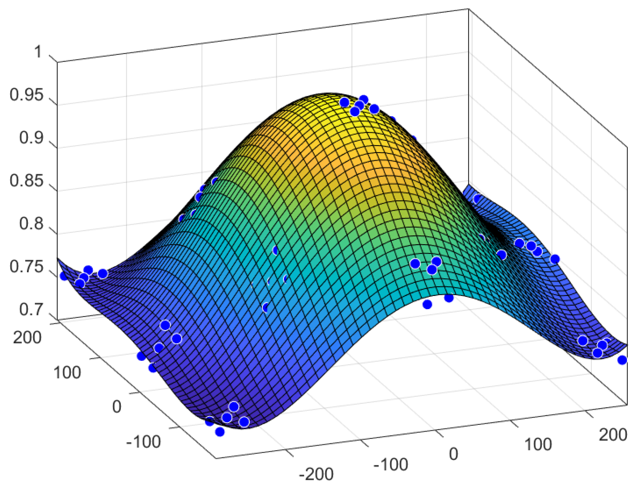
2.3.3. Vignetting

To characterize vignetting, a white target was imaged, as shown in Figure 3. The camera was rotated to orientate the target at 13 positions within the camera’s FOV, and 5 readings were extracted for each orientation for a total of 65 readings. Vignetting dimming at a position was assessed as the ratio of readings at each position to the central position. As the form for this lens was unknown, a generic fifth-order 2D polynomial was fit for vignetting dimming against the pixel location. This polynomial is defined in (x, y) as follows:

V(x,y) = a + b·x + c·y + d·x² + e·xy +f·y² + g·x³ + h·x²y + h·xy² + i·y³ + j·x⁴ + k·x³y + l·x²y² + m·xy³ + n·y⁴ + o·x⁵ + p·x⁴y + q·x³y² + r·x²y³ + s·xy⁴ + t·y⁵

(3)

2.3.4. Low-Cost Absolute Luminance Calibration

For luminance characterization, a unique relationship between HDR pixel color measurements (r, g, b) corresponding to the k-value for each color channel and luminance (L) is found by creating a new set of coefficients (C_r, C_g, C_b), such that

L = C_r·r + C_g·g + C_b·b

(4)

To find these new coefficients, camera color intensity readings and corresponding luminance measurements are recorded for a range of colored targets. The camera and a Hagner Luminance meter were set up as in Figure 3 with colored targets, as shown in Figure 4. The targets were imaged following the process outlined in Section 2.3.1, and a 7 × 7 array of manual luminance readings were taken of each colored target to capture the distribution of luminance across targets. These luminance readings and corresponding HDR pixel intensities (r, g, b) were used to fit Equation (4) for C_r, C_g, and C_b using least squares regression.

2.3.5. Ultra-Low-Cost Relative Luminance Calibration

Similar to absolute luminance calibration, the measurement device is calibrated instead to relative luminance (rL) by fitting a new relationship between imaged color target digital values and meter readings and generating a new set of coefficients (Ĉ_r, Ĉ_g, Ĉ_b):

rL = Ĉ_r·r + Ĉ_g·g + Ĉ_b·b

(5)

where rL is the relative luminance and r, g, b are the HDR pixel intensities.

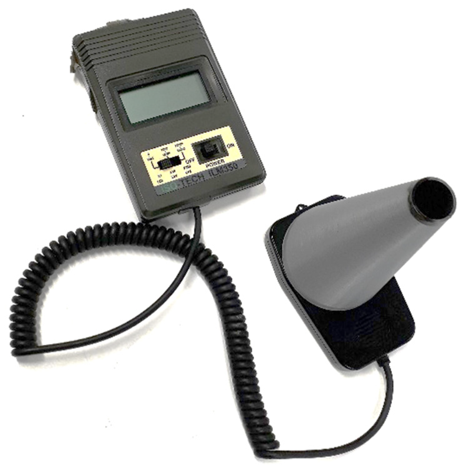
Relative luminance readings are taken by transforming a common illuminance meter into a relative luminance spot meter by fitting a cone to narrow the aperture, as shown in Figure 5. The internal surface of the cone was painted black to reduce internal reflections. This follows a similar method demonstrated in Cuttle’s “Lighting Design—a perception based approach” [46] for measuring reflectance values.

This approach to measuring relative luminance works, as luminance (L) and illuminance (E) are related by the solid angle (Ω) of light radiated, expressed as follows:

E = ∫L·dΩ

(6)

where the geometry (Ω) is held constant and relative luminance would be found by the ratio between any two illuminance readings (points 1 and 2), expressed as follows:

rL = L₁/L₂ = E₁/E₂

(7)

Fitting the cone reduces the aperture and limits the reading to a “spot” of interest.

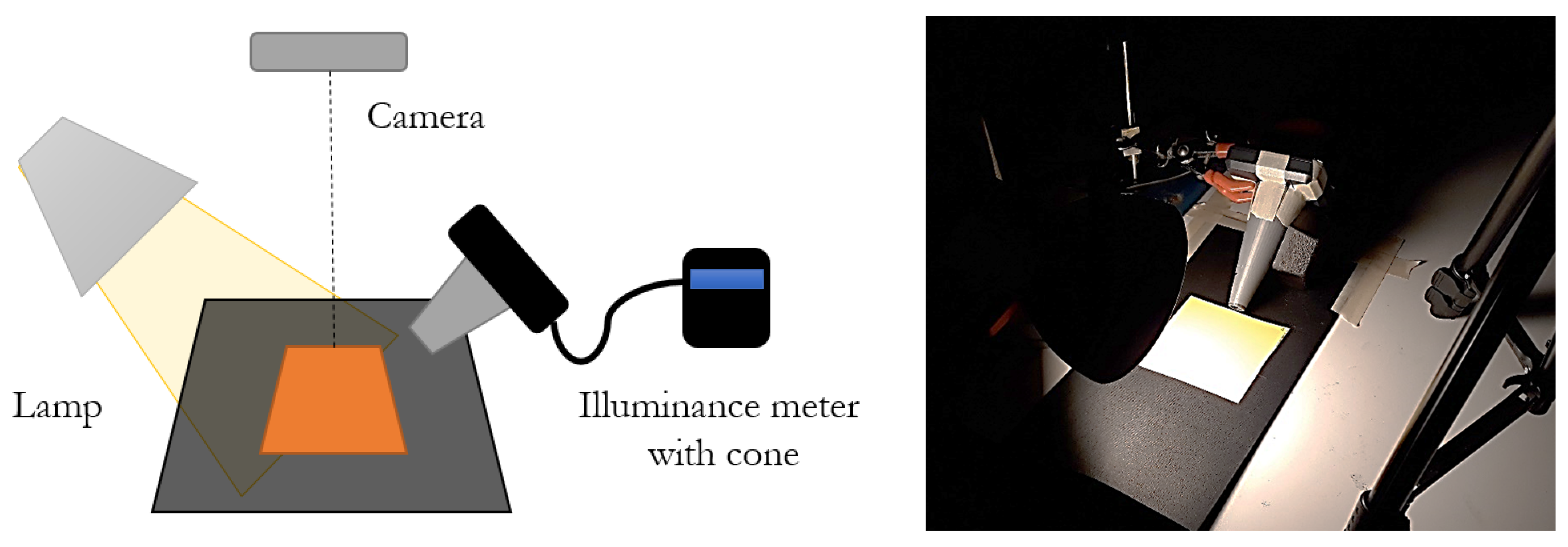
Spot relative luminance readings and images are taken of a series of illuminated colored targets, paint swatches. Seven colors ensure accuracy across a broad color range. The experimental setup is shown in Figure 6. Each color target was imaged in turn under constant illumination with an incandescent bulb providing full-spectrum non-flickering illuminance. The relative geometry was unchanged between measurements. Average color intensity readings were extracted from HDR images, and along with the manual relative luminance readings, Equation (5) was fit using least squares regression to derive a new set of coefficients.

2.3.6. Device Measurement Range

Device measurement range is limited by pixels reaching saturation at very low exposure speeds, where increased light gives no additional response, and the device becomes inaccurate. To assess maximum measurable luminance, the highest pixel intensity (k_s) is extracted from the pixel response image, shown in Figure 2. Maximum luminance is color dependent as luminance depends on color per Equation (4). To represent device measurement limits across a range of colors, color readings for absolute luminance calibration, as shown in Figure 4, are scaled up until one value reaches the maximum pixel intensity (k_s). The resultant HDR color values are applied to Equation (4) to give luminance values. The output is a maximum measurable luminance value for each color target (red, blue, green, and yellow).

2.4. Performance Analyses

Experimental tests assessing pixel response model fit, vignetting model fit, absolute luminance, and relative luminance accuracy are compared to specifications in Table 1. Specifically,

• Pixel response model fit is assessed as average R² correlation or goodness of fit across the FOV;
• Vignetting model fit is assessed as mean percentage error over FOV vs. specification of ≤2%;
• Absolute luminance accuracy over the FOV is assessed as an average and peak error percentage vs. specification of <7% and an acceptable higher value of <10%;
• Relative luminance accuracy over the FOV is assessed as an average and peak error percentage vs. specification of <7% and an acceptable higher value of <10%;
• Device measurement range is assessed as an absolute measurement range vs. a specification of ≥1–1 × 10⁵ cd/m².

Where “Accuracy over the FOV” is assessed as a simple sum of average and peak errors for vignetting and color-to-luminance calibration, respectively.

2.5. Demonstration—Measurement of Discomfort Glare

The custom device, calibrated to absolute luminance, is demonstrated for the application of measuring glare. An office scene with overhead lighting was imaged, shown in Figure 7. The scene is representative of where discomfort glare is likely to occur and where the evaluation of discomfort glare is useful. Once the absolute luminance map for the scene was acquired, the glare sources were isolated, and discomfort glare was calculated by summing the contributions of each pixel to discomfort glare, evaluated as Unified Glare Rating (UGR) [47].

UGR = 8log₁₀[0.25/L_B ∑ L_Sn² Ω_n/p_n²]

(8)

where L_B is the luminance of the background of the scene with lamps excluded, L_Sn is the luminance of the nth light source, Ω_n is the solid angle of the nth light source, and p_n is the Guth position index of the nth light source. In this case, light sources are simply the pixels of any light source. The Guth position index [38] reflects the human viewer’s sensitivity to discomfort glare for different positions in the FOV and is defined as follows:

p = exp(35.2 − 0.31899α − 1.22e^−2α/9)10⁻³β + (21 + 0.26667α − 0.002963α²)10⁻⁵β²

(9)

where α and β are the vertical and horizontal angles from the line of sight to the light source in degrees.

3. Results

3.1. Pixel Response

The pixel response model was applied to the calibration image of Figure 3. The average R² goodness of fit across the image was above R² > 0.97, and 99% of the pixels exceeded a fit of R² > 0.94. Figure 8 demonstrates the pixel response quality of fit, with a good model fit of R² = 0.99 and a poorer fit of R² = 0.94. The pixel intensity values are then found using Equation (10):

k = (1/es)tanh⁻¹(DV/240)

(10)

This hyperbolic tangent model was compared to a model fit with a simple power law, which resulted in a lower average goodness of fit of R² = 0.78.

3.2. Vignetting

Equation (11) was identified for lens vignetting (V) with an accuracy over R² = 0.99. The model fits well, with an average error of 1.5% over the 65 points assessed across the FOV, and a maximum difference of 4% observed at the edges of the image. Figure 9 shows the readings and model fit; the z-axis is off-axis dimming as a ratio of off-axis to central readings.

V(x,y) = 0.993 − 0.000174x + 0.0002267y − 5.73 × 10⁻⁶x² − 1.26 × 10⁻⁷xy − 4.383 × 10⁻⁶y² + 2.138 × 10⁻⁹x³ + 1.402 × 10⁻⁹x²y + 5.075 × 10⁻⁹xy² − 5.962 × 10⁻⁹y³ + 3.919 × 10⁻¹¹x⁴ + 3.732 × 10⁻¹²x³y + 4.2 × 10⁻¹¹x²y² − 2.281 × 10^—12xy³ + 2.571 × 10⁻¹¹y⁴ + 1.69 × 10⁻¹⁴x⁵ + 1.186 × 10⁻¹⁴x⁴y − 4.437 × 10⁻¹⁴x³y² + 2.019 × 10⁻¹⁴x²y³ − 2.611 × 10⁻¹⁴xy⁴ + 3.047 × 10⁻¹⁴y⁵

(11)

3.3. Absolute Luminance Calibration

The fitting procedure for absolute luminance gave a set of three new coefficients:

C_r = 724649, C_g = 2970612, C_b = 0

(12)

Equation (12) yields R² = 0.98. The readings normalized to the green channel yield are as follows:

C_r = 0.244, C_g = 1.00, C_b = 0

(13)

The average error across colored targets was 4.9%, and the maximum error was below 5.4%; the camera predicted luminance readings and luminance meter readings for each target, and the relative and absolute errors are listed in

Table 3. Summarizes the Hagner luminance meter readings, camera-measured luminance, and corresponding errors for each colored target.

Target	Fit Luminance (cd/m2)	Luminance Readings (cd/m2)	Error (%)	Absolute Error (cd/m2)
Blue	73.5	69.8	5.3	3.7
Green	123	128	3.7	4.7
Yellow	173	183	5.3	9.7
Red	60	57	5.3	3.0

. Considering the vignetting error, the resultant total error over the FOV is 6.4% and 9.4%, for average and peak error, respectively.

3.4. Relative Lumiance Calibration

The relative luminance procedure gave a new set of coefficients with the coefficients normalized to the green coefficient yielding an accuracy of R² = 0.96, and are defined as follows:

Ĉ_r = 0.232, Ĉ_g = 1.000, Ĉ_b = 0.000

(14)

To verify this approach, these coefficients were applied to the HDR images captured for the absolute luminance calibration, Section 2.3.4, and compared to the corresponding luminance measurements. The values were scaled with a minimum error approach to compare relative and absolute luminance readings.

Table 4. Summary of the fit luminance values, which are the scaled relative luminance measurements taken from the camera, and the corresponding absolute luminance readings from the Hagner luminance meter.

Target	Fit Luminance (cd/m2)	Luminance Readings (cd/m2)	Error (%)	Absolute Error (cd/m2)
Blue	73.5	69.8	5.6	3.9
Green	123	128	3.7	4.7
Yellow	173	183	5.6	10.2
Red	60	57	3.8	2.2

summarizes the results and errors. There was a maximum error of 5.6% and an average of 4.7% for the targets. Considering the vignetting error, the resultant total error over the FOV is 6.2% and 10.6% for average and peak error, respectively.

3.5. Device Luminance Measurement Range

Device measurement upper limits for a range of colors are summarized in

Table 5. Summary of the approximate maximal measurable luminance values across a set of colored targets.

Target	Highest Measurable Luminance (cd/m2)
Blue	92,882
Yellow	104,643
Green	96,420
Red	54,288

. One target exceeds the specification of 1 × 10⁵ cd/m^2, and two more are within 10%. The red target is lower than the specification by nearly a factor of 2.

3.6. Demonstration of the Measurement of Discomfort Glare

Discomfort glare, defined as the UGR, was calculated using the absolute luminance map for the scene imaged in Figure 7. Figure 10 displays the luminance map with glare sources isolated.

The UGR was evaluated to be 21.1.

UGR = 21.1

(15)

4. Discussion

4.1. Pixel Response

The pixel response characterization had a high degree of accuracy, with an average fit of R² = 0.97 across the calibration image. The hyperbolic model had minimal error. For comparison, a simple power-law model had a much lower goodness of fit of R² = 0.78. Overall, the procedure works well and shows that low-cost and highly non-linear sensor responses may be accurately linearized and provide accurate measurements across a wide range of light levels.

Due to observed variability, digital values below 10 and above 230 were filtered, reducing the overall measurement range and removing very dark readings and very bright readings. The remaining variability in the model is due to sensor noise, which is higher in lower-quality sensors. Thus, a greater quality fit and, consequentially, a further reduction in device measurement error could be found with higher-quality sensors.

4.2. Vignetting

The vignetting model was fit within specification to an accuracy of R² = 0.99, with an average error over the FOV of 1.5% and a peak error of 4% at the image periphery. This quantification of vignetting agrees well with another study characterizing vignetting for the OV5647 sensor module under uniform illumination conditions [21]. The error could be reduced by taking more readings and eliminating light sources at extreme angles, such as overhead lights. While not in the FOV, bright sources still affect readings by scattering light within the lens [15]. This outcome shows this very simple and virtually no-equipment procedure may be used to quantify vignetting with accuracy allowing accurate measurements across a camera’s whole FOV.

4.3. Absolute Luminance Calibration

Absolute calibration luminance calibration was performed without using uniform sources against a Hagner S4 luminance meter to an average error of 4.9% and peak error of 5.3%, or 6.4% and 9.4% for the total error across the FOV, which considers the vignetting error, which is below the 7% specification. This device error falls within the range reported for custom luminance cameras of 5–12%. These results demonstrate it is possible to obtain a sufficiently accurate luminance calibration without uniform lighting sources and the associated expenses.

4.4. Relative Luminance Calibration

Relative luminance calibration resulted in an average error of 4.7% and peak errors of 5.6%, or 6.2% and 10.6% for the total error across the FOV, which considers vignetting. These values are within the specification and in the range found by other researchers for custom luminance measurement devices [11,12,13,14,15,16,17,18,21].

This procedure calibrates to relative luminance instead of absolute luminance and thus removes the need for expensive luminance meters, removing a significant barrier to adopting luminance imaging. Illumination meters are lower cost and commonplace as they are required in compliance with many lighting guidelines and standards [37,38,48]. As such, requiring only illuminance meters makes this procedure more useful in the current technical environment.

However, relative luminance imaging has limitations, as many useful lighting metrics, such as glare (UGR) [37,38] and visual performance [10,49], require absolute luminance measurements, which limits the utility of this device and procedure. However, alternative simplified measures exist for key lighting metrics which could make relative luminance imaging useful [21,50], such as luminance ratios for aesthetics (visual–interest ratio) and glare [38,39]. These approaches would be suitable for this device.

4.5. Device Measurement Range

The upper limit for device luminance measurement, as the determinant of measurement range, was assessed across a range of colored targets. The device exceeded the 1 × 10⁵ cd/m² specification only for the yellow target at 1.05 × 10⁵ cd/m². Two targets (blue and green) were close to, but under, the specification at 9.6 × 10⁴ cd/m² and 9.3 × 10⁴ cd/m², respectively. The red target was far lower than the specification, at 5.4 × 10⁴ cd/m².

While only a single target exceeded specification, the result is still favorable for practical use for two reasons: (1) the green and blue targets are sufficiently close to specification, and (2) the yellow target, which exceeds specification, is a better representative of high luminance encountered in indoor luminance environments, such as artificial lamps or direct sunlight. Conversely, high luminance highly saturated red colors are uncommon in indoor environments, so it is unlikely they will reach the device limit. If the device’s range is exceeded, the results may still be useful, as a lower estimate of environmental luminance could still be used. In the case of glare assessment, where high luminance levels are most likely to occur and hence most likely exceed device specifications and saturate the sensors, the device range limit will impose a limitation. However, the results are still useful: while they do not provide an exact evaluation of glare, they do indicate a minimum glare level.

This overall result demonstrates low-cost imaging devices have sufficient range for indoor lighting applications. To increase device range, a neutral density filter could be employed to reduce the light reaching the sensor by a known factor. Alternatively, a device with a lower minimum shutter speed may be employed. For instance, modern smartphones such as the Samsung Galaxy S21 series [51] support framerates as high as 960 fps for slow-motion video capture. For reference, 960 fps corresponds to an over 11-fold increase in upper device measurement limit compared to the RPi camera module, and far exceeds indoor lighting analysis requirements.

4.6. Luminance Calibration Models

Both the relative and absolute luminance calibration models used a linear combination of the three color channels, corresponding to the known color-to-luminance relationship in Equation (1). However, the model does not account for sensor noise arising from electrical cross-talk and thermal radiation, among other factors. These external factors can be grouped into a ‘dark frame’ or ‘dark noise’ term published by manufacturers [42,52]. As such, additional terms could be added to the calibration models to account for this effect and increase accuracy.

4.7. Calibration Equipment and Costs

The device and calibration procedures described in this research present significant cost reductions compared to existing commercial devices and calibration procedures. The base device was a low-cost Raspberry Pi microcomputer (~USD 60). The pixel response characterization procedure used only exposure speed variation, eliminating the need for calibrated light sources and allowing the use of low-cost sensors. This minimal equipment vignetting calibration accurately characterized vignetting over the FOV and eliminated the need to use uniform fields. The absolute luminance and relative calibration procedures utilized only a luminance meter and an illuminance meter, respectively. These devices have approximate costs of ~USD 3000 for the luminance meter [53] and USD 600 for a high-quality illuminance meter [54], significantly reducing costs and barriers to adoption.

4.8. Demonstration–Measurement of UGR

The device was demonstrated with the measurement of discomfort glare for a common office scene with many overhead lamps, which is representative of a scene likely to cause discomfort glare. The device successfully evaluated a UGR for this scene as 21.1. This value for glare is high but not unreasonable; typical indoor recommendations for offices range between 16 and 22 [37]. The successful evaluation of the UGR with low-cost devices demonstrates the utility of such devices to practitioners, as the UGR is a common and important lighting metric.

4.9. Limitations

A key limitation, as for other researchers who have produced custom devices, is the lack of comprehensive error analysis, which may reveal higher errors or weak points in these devices or calibration procedures. Typically, the error is assessed against another device, which carries its own error, for a select number of colored targets. However, as the error can depend on target color, target distance, location in the FOV, and luminance range, meaningfully assessing and completely characterizing device accuracy is difficult.

In both the absolute and relative luminance calibration methods, the blue coefficient (C_b) was identified as zero. Despite losing a parameter in the proposed model, overall accuracies were within specifications. The blue coefficient is expected to be small where color measurement is accurate, per Equation (1). All targets imaged had very low or zero blue-channel readings, likely due to lower light transmission of the blue filter in the Bayer array and the filtering of low values (DV < 10), which removed the effect of the blue channel. This issue could be rectified by increasing the overall target illumination, and could further reduce errors.

The calibration procedures can be time intensive, particularly the manual image processing required to extract values. However, this process is also an excellent candidate for software automation, as it fits existing image recognition capabilities. Automation would allow the rapid characterization of multiple devices, lenses, and lens additions, such as fish-eye lenses.

Currently, the device is not optimized for speed; the imaging device developed requires substantial time to capture (~30 s) and process (~3 m) images. Image acquisition time is dependent on the number of images and exposure times. To reduce image acquisition time, the range of exposure times taken may be optimized, eliminating unnecessary exposures and balancing luminance measurement accuracy. Image acquisition optimization could be a dynamic process, adjusting exposure speeds captured with environmental light levels. Fewer images also reduce HDR image processing time.

Overall, the device error for the very low-cost solution presented exceeded specification. However, increased accuracy may be required for complex lighting measures, where luminance error compounds. Higher-quality sensors can give higher accuracy. Increasing numbers of smartphones have very high imaging capacity and on-board processing compared to the very simple device presented. Smartphone-based luminance imaging could further decrease costs and increase measurement accuracy due to their increasingly high-quality imaging sensors.

Outside of reducing device error, the effect of device error on key lighting measure error could be reduced by using alternative formulations where the error does not compound. In the case of glare, alternative and simpler metrics exist, such as luminance ratios [38,49]. The simple ratios include fewer luminance terms, so the glare measurement has a lower total error, which reduces the impact of higher device measurement error in low-cost devices.

4.10. Practical Implications

The low-cost and minimal equipment procedures laid out for absolute and relative luminance calibration worked well with minimal error, comparable to devices not subject to the same constraints. Thus, luminance and relative luminance imaging can be accurately achieved at a very low cost using only a luminance meter or commonly held illuminance meter for calibration. By addressing the significant equipment and cost barriers to luminance imaging, these procedures open the door to widespread luminance imaging for real-time evaluation of illumination and lighting comfort and performance [1], which can aid in the design, tuning, and control of artificial and natural lighting.

This work could be extended for smartphone-based luminance imaging, which would eliminate device costs. Smartphone processing and camera sensors exceed the specifications of the RPi and camera sensor used in this research. However, the accessibility to key camera settings would need to be assessed.

5. Conclusions

A luminance imaging device was developed using a low-cost device and sensor, and minimal calibration equipment. The device demonstrated accuracy comparable to other custom devices using higher cost technologies and more extensive calibration equipment, and is accurate for indoor lighting measurements. There is still room for improvement; several means to further improve device accuracy and measurement range have been suggested. This work demonstrates accurate luminance imaging can be achieved at a very low cost with minimal equipment.

Minimal equipment procedures were developed to characterize pixel response and vignetting. A no-equipment calibration procedure was developed, which can effectively linearize highly non-linear sensors. This procedure enables the use of affordable sensors with a highly non-linear response, for luminance imaging, instead of high-cost alternatives with a linear response. A minimal equipment process was developed to characterize vignetting, which required only a steady light source instead of uniform luminance fields achieved with high-cost integration spheres and luminous ceilings. The procedures outlined remove the need for expensive and economically inaccessible calibration equipment and lower device and calibration costs.

Further improvements to this device can be obtained by utilizing increasingly common smartphone technologies. Even affordable modern smartphones have imaging capacities, with high-quality sensors, a range of shutter speeds, and on-board image processing, which far surpass the device used in this research. Integrating the imaging techniques developed in this research into a smartphone app could utilize these still rapidly increasing imaging capacities, increasing accuracy and performance. Considering many people already own a smartphone, device costs could be effectively eliminated, reducing total costs while using their computational capacity to enable automation of the calibration procedures presented.

Lowering the cost of luminance imaging removes a significant barrier to adopting luminance-based lighting metrics. Luminance-based lighting measures are closer to how we see, and allow for the direct evaluation of many aspects of visual performance through metrics such as RVP [55] and visual comfort [1]. Overall, adopting luminance-based measures would lead to better, more efficient, and high-performing lighting design.