Exploring the Impact of Different Registration Methods and Noise Removal on the Registration Quality of Point Cloud Models in the Built Environment: A Case Study on Dickabrma Bridge

Abstract

Point cloud models are prevalently utilized in the architectural and civil engineering sectors. The registration of point clouds can invariably introduce registration errors, adversely impacting the accuracy of point cloud models. While the domain of computer vision has delved profoundly into point cloud registration, limited research in the construction domain has explored these registration algorithms in the built environment, despite their inception in the field of computer vision. The primary objective of this study is to investigate the impact of mainstream point cloud registration algorithms—originally introduced in the computer vision domain—on point cloud models, specifically within the context of bridge engineering as a category of civil engineering data. Concurrently, this study examines the influence of noise removal on varying point cloud registration algorithms. Our research quantifies potential variables for registration quality based on two metrics: registration error (RE) and time consumption (TC). Statistical methods were employed for significance analysis and value engineering assessment. The experimental outcomes indicate that the GRICP algorithm exhibits the highest precision, with RE values of 3.02 mm and 2.79 mm under non-noise removal and noise removal conditions, respectively. The most efficient algorithm is PLICP, yielding TC values of 3.86 min and 2.70 min under the aforementioned conditions. The algorithm with the optimal cost-benefit ratio is CICP, presenting value scores of 3.57 and 4.26 for non-noise removal and noise removal conditions, respectively. Under noise removal conditions, a majority of point cloud algorithms witnessed a notable enhancement in registration accuracy and a decrease in time consumption. Specifically, the POICP algorithm experienced a 32% reduction in RE and a 34% decline in TC after noise removal. Similarly, PLICP observed a 34% and 30% reduction in RE and TC, respectively. KICP showcased a decline of 23% in RE and 28% in TC, CICP manifested a 27% and 31% drop in RE and TC, respectively, GRICP observed an 8% reduction in RE and a 40% decline in TC, and for FGRICP, RE and TC decreased by 8% and 52%, respectively, subsequent to noise removal.

1. Introduction

Point cloud models have an extensive range of applications within the Architecture, Engineering, and Construction (AEC) industry, such as building maintenance management, building refurbishment and modification, as well as structural health monitoring [1,2,3,4,5]. The term “point cloud model” refers to a collection of 3D points, each of which is characterized by x, y, z coordinates, used to represent the information on various objects or components [6,7,8]. Typically, these 3D points also encompass RGB data, providing color information for the depicted component [9].

Point cloud data can be gathered using various reality capture technologies, including laser scanning and digital photogrammetry. Laser scanning technology can be further subdivided into Terrestrial Laser Scanning (TLS) and Mobile Laser Scanning (MLS) technologies. TLS, which involves stationary scanning, is characterized primarily by offering superior precision, capturing point cloud data with higher resolution and density [7,10,11,12,13]. While MLS may not match TLS in terms of precision and density, it offers greater flexibility, enabling the scanning of complex architectural environments [14]. It provides excellent solutions for addressing architectural blind spots that TLS might not be able to cover [15,16,17,18,19]. Digital photogrammetry, in contrast to laser scanning techniques, is known as a passive reality capture technology. It does not actively emit any laser beams or signal waves. Instead, it passively captures reflected light from natural or artificial light sources on objects through photodetectors to form images. Then, algorithms such as Structure from Motion (SFM) are employed to reconstruct the three-dimensional information corresponding to the pixel values in the photographs [20,21,22,23]. Compared to laser scanning techniques for point cloud data collection, digital photogrammetry offers lower accuracy and point cloud density, and it cannot perform reality capture in dark environments [24]. However, its hardware equipment is considerably more cost-effective than that utilized in laser scanning methods [23].

Upon the completion of point cloud data collection, the raw data must undergo a series of processing steps to form a point cloud model. These processes include noise removal, subsampling, and registration, among others [7,13]. Of these, registration is arguably the most crucial step. Typically, a project is large, and it is unlikely that a single scan can cover all the data required. Additionally, multiple devices may be used together, each performing its own point cloud data collection, with the data existing in an independent coordinate system [25,26]. To generate a comprehensive point cloud model, it is necessary to accurately synthesize the data from different parts of the project into a common coordinate system using appropriate point cloud registration methods. However, the registration process may not always be straightforward. Significant registration errors can lead to a decrease in the overall accuracy of the point cloud model. Even minor errors can gradually accumulate into larger ones throughout multiple continuous scans and iterative registration processes, thereby impacting the overall accuracy [27,28]. This is especially pertinent in bridge engineering, which often involves many successive and adjacent scans in the same direction. Even the slightest errors can iterate into substantial ones, potentially causing significant discrepancies.

Data in the built environment possesses distinct characteristics. Conducting in-depth research on the point cloud registration algorithms proposed in the field of computer vision, specifically within a built environment context, facilitates for construction professionals the crafting of superior point cloud models, thereby better aligning with application scenarios in the construction industry. However, in the current construction industry, few teams have explored point cloud registration algorithms, proposed in the computer vision domain, in specific architectural contexts. The primary objective of this research is to investigate the impact of different registration methods and the role of noise removal on the quality of point cloud registration. This study quantifies registration quality through two metrics: Registration Error (RE) and Time Consumption (TC). Furthermore, all registration methods tested in this experiment are evaluated using the value engineering method, with the goal of identifying the registration method that offers the highest cost-effectiveness. Through this experimental study, the authors aim to provide empirical data support to scholars and practitioners in the construction industry when establishing high-precision point cloud models within the built environment. Based on the results of this investigation, readers can gain a comprehensive understanding of the performance of mainstream point cloud registration methods in bridging construction, as well as the extent to which noise removal can impact registration quality.

2. Related Work

2.1. Registration Method

Registration methods can generally be subdivided into two distinct categories: coarse registration and fine registration [28,29,30,31]. The primary objective of coarse registration is to establish an approximate initial alignment of the source and target point cloud that are to be registered. This alignment, which ideally should result in a general overlap of the two point clouds, consequently influences the precision of the subsequent fine registration process. There are primarily three strategies employed in coarse registration. The first strategy is the manual method, which necessitates human intervention. In this method, corresponding points or surfaces are selected from both the source and target point clouds, after which point pairs are formed and used for registration [32]. The second strategy is the target-based method. During the registration process, markers are placed, which are then identified in both the source and target point clouds. This method facilitates the formation of point pairs from corresponding markers [8]. The third strategy is descriptor-based. In this method, descriptors of both the source and target point clouds are computed, and point pairs are formed from points with identical descriptor features for registration [26,33,34].

Fine registration, on the other hand, is conducted after the completion of the coarse registration process. Its purpose is to fine-tune the alignment of the source and target point clouds to achieve an optimal overlap. The accuracy of the point cloud ensemble formed from the two point clouds can be affected by error in the fine registration [28]. The methodologies for fine registration are primarily Iterative Closest Point (ICP) and its derivative algorithms [35,36]. These algorithms are characterized by initial position, thresholds, loss function, and iteration. Throughout the iterative process, the loss function is manipulated to meet the threshold requirements, ultimately leading to the final transformation matrix [25].

2.2. Noise and Outlier Removal

Noise and outliers both represent data characteristics that negatively impact the accuracy of point cloud models [37]. Outliers are defined as points with exceptionally large error values, far exceeding systematic errors and caused by complex and special factors. The presence of these points is determined by numerous factors, such as the material, color, roughness of the scanned object, and environmental conditions, such as temperature and lighting intensity [10,38,39]. Outlier detection and removal in data has been extensively studied, employing diverse methodologies. Prominent approaches predominantly utilize local statistics to determine anomalies, referencing metrics like local density [40], proximity to nearest neighbors [41], and eigenvalues of the local covariance matrix [42], with further methods catalogued by Papadimitriou et al. [43]. While some methods opt for direct hard thresholding to identify outliers [41], others prefer a distributional approach, commonly assuming a normal distribution, to highlight deviant points [40]. Moreover, there is a distinction in literature between sparse outliers and temporal artifact outliers, the latter often associated with scene movements. For instance, Kanzok et al. [44] focused on filtering out such temporal artifacts by identifying transient clusters.

On the other hand, noise refers to a uniform, systematic error inherent in the process of data collection via laser scanning technology. This type of error is ubiquitous and cannot be compensated for through hardware optimization. Certain non-target objects can also be considered a specific type of noise. During the scanning process, the resultant point cloud data often encapsulates objects irrelevant to the target object. For instance, when scanning a building structure, the collected point cloud data may also incorporate flora, fauna, pedestrians, and birds [45]. These elements typically exhibit non-static properties and can obstruct the target objects to a certain extent [7]. In the realm of point cloud data processing, noise removal stands out as a pivotal challenge, given the intricate balance between filtering out extraneous noise and preserving crucial, sharp features. Foundational techniques, like local neighborhood smoothing, provide a basis, but often risk over-smoothing. The kernel density estimator, as noted by Schall et al. [40], showed potential, but faltered near sharp regions. Iterative sampling, explored by Liu et al. [46], filled data holes adeptly but struggled with feature restoration. The literature revealed a trend towards anisotropic filtering, which adjusts smoothing based on directionality, with Lange and Polthier [47] introducing a method using mean curvature flows, though it is computationally demanding. An evolution of this, presented by Wang et al. [48], targeted point normal for more efficient results. Interestingly, some other researchers, such as Ahmed et al. [49] and Aiger et al. [31], circumvented filtering, aiming for inherent noise robustness. Tools like PCL, Open3d, CloudCompare, and MeshLab encapsulate these advancements, offering practical solutions for researchers and practitioners.

2.3. The Importance of High-Quality Point Cloud Models

The escalating integration of point cloud models into modern engineering and architectural applications accentuates the pivotal role of their accuracy and precision. Most research concerning the accuracy of point cloud models predominantly elucidates the implications of varying precision levels from an application-oriented perspective.

In the evolving landscape of construction quality inspection, point cloud models act as a mirror, reflecting the real-world status of ongoing construction projects. They offer an unparalleled medium to juxtapose the on-ground construction with as-designed BIM models. This comparative analysis facilitates the evaluation of adherence to design standards, detection of discrepancies, and ensures that the on-site work aligns with the preconceived design blueprints [50]. A compromise in the fidelity of point cloud models can result in erroneous evaluations, thereby potentially jeopardizing the integrity of the entire construction project [51,52].

The Scan-to-BIM methodology underscores the significance of point cloud models. A large swathe of extant structures, with legacy documentation or even lacking detailed plans, necessitates the creation of high-precision point cloud models. These models serve as the foundational layer for developing digital twin replicas, which aid in visual asset management, structural health assessments, and future retrofitting plans. An imprecise point cloud model might lead to the formulation of a digital twin that veers away from reality, limiting its applicability in real-time simulations and analysis [53,54,55].

Point cloud models play a linchpin role in contemporary renovation and remodelling tasks. The ability to digitize an existing structure with high precision provides architects and designers with an accurate canvas, which becomes the basis for their redesign initiatives. A lackluster accuracy in point cloud models could stymie the planning phase, culminating in redesigns that might be unfeasible or in dissonance with the actual structure [1,56].

High-quality point cloud models are not a luxury but a quintessential need in today’s technologically-driven architecture and engineering landscapes. Their precision dictates the success of a myriad of applications, making their accuracy a non-negotiable attribute for professionals in the field.

3. Methodology and Experiment

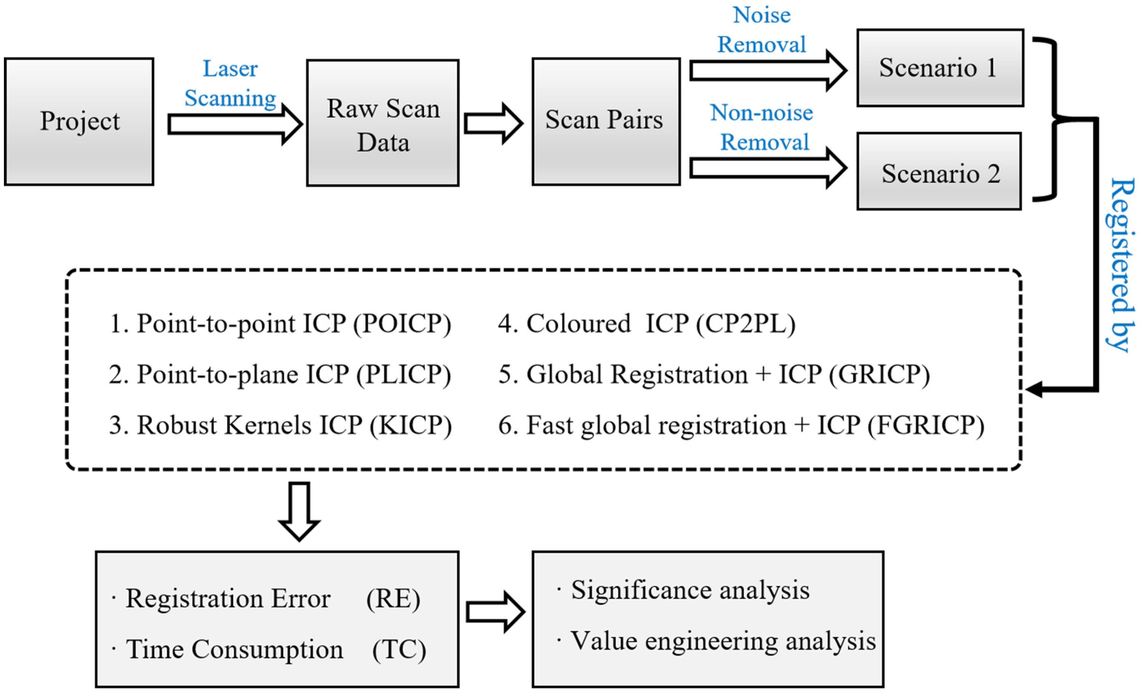
3.1. Framework

The primary aim of this study is to investigate the impact of different point cloud registration strategies and the potential influence of noise removal on the quality of point cloud registration. The entire exploration process encompasses five steps (Figure 1). Firstly, we collected data on the target bridge structure using a terrestrial laser scanner. Secondly, the original point clouds, or scans, were divided into several scan pairs according to the rule of pairing adjacent scans. Each scan pair consists of a source point cloud and a target point cloud. Thirdly, we established two scenarios. Scenario 1 involves raw scan pairs, meaning no additional processing is performed. Scenario 2 involves noise removal processing on the basis of raw scan pairs, deleting all point clouds irrelevant to the main body of the bridge, primarily including trees, plants, pedestrians, and vehicles. Fourthly, we applied six different point cloud registration algorithms to register the scan pairs in the two scenarios, and then obtained the RE data and the time TC data for each scan pair. Finally, we employed significance analysis and value analysis to process and analyze the RE data and TC data.

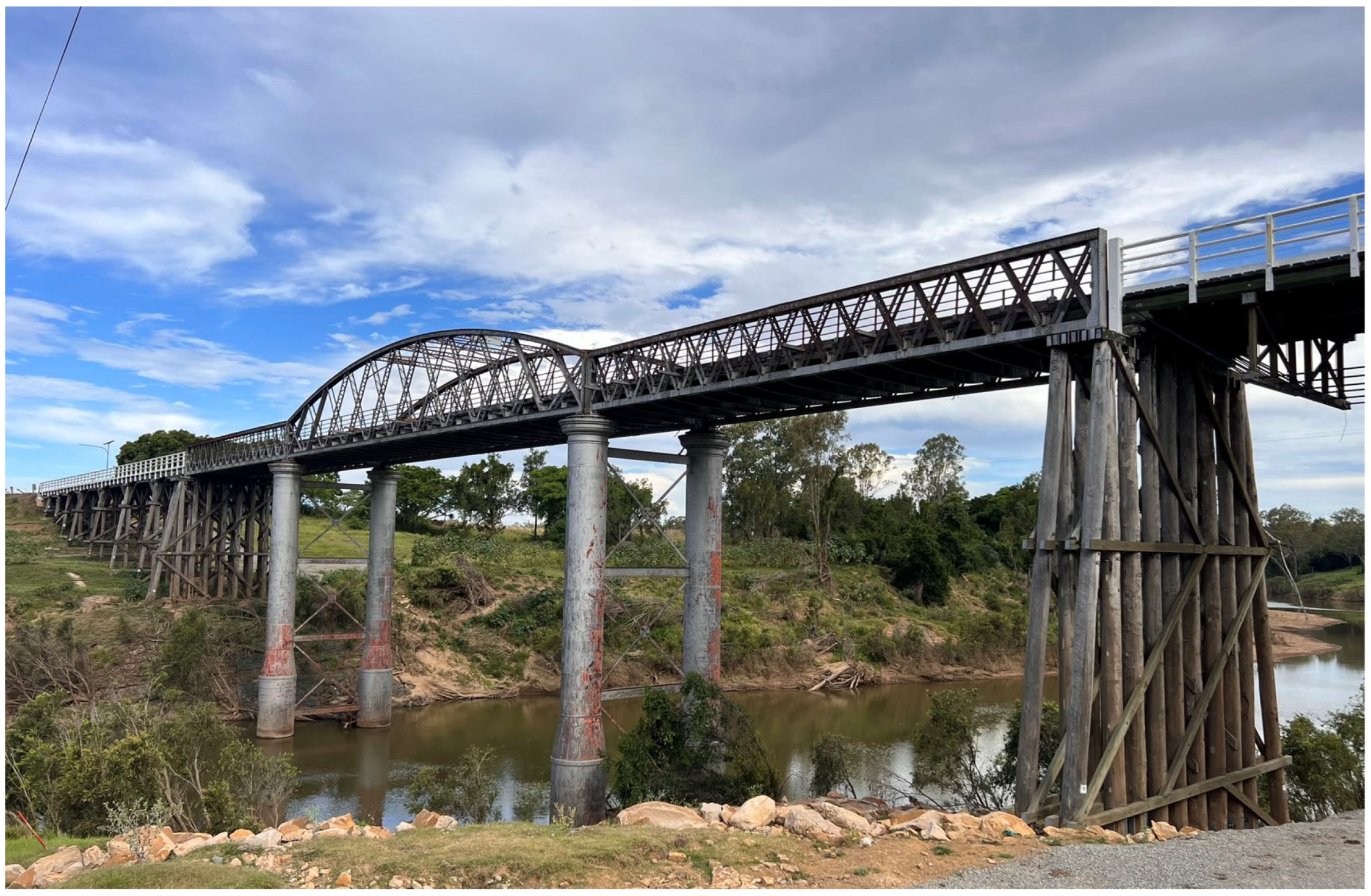
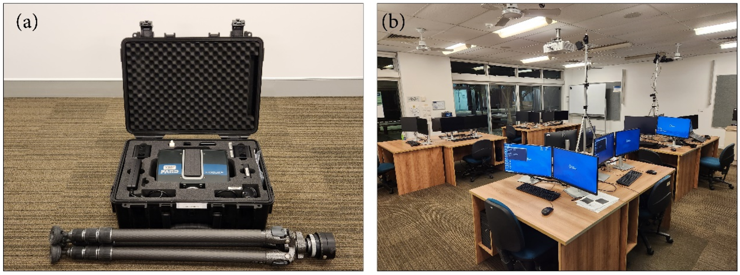
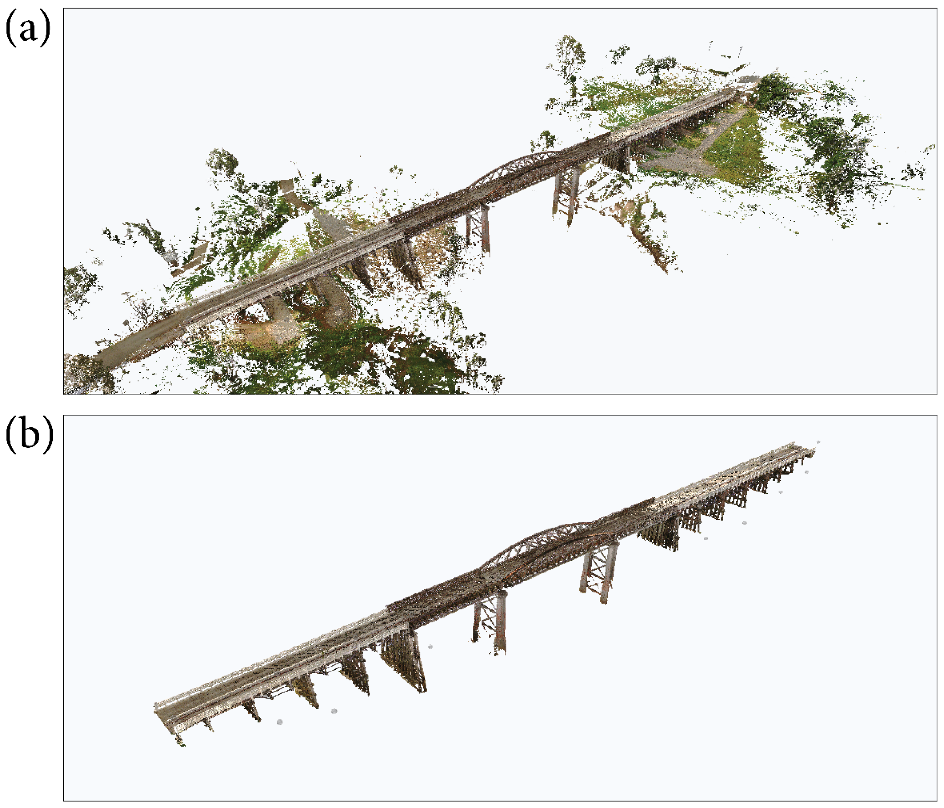
3.2. Project and Equipment

The Dickabram Bridge (Figure 2), a significant historical road-and-rail bridge over Australia’s Mary River, connects the towns of Miva and Theebine in the Gympie Region, Queensland. The bridge, known also as Mary River Bridge (Miva), is notable for being a primary structure on the Kingaroy railway line. Its construction, from 1885 to 1886, was overseen by Henry Charles Stanley, with building duties carried out by Michael McDermott, Owens & Co. This structure was recognized for its national importance and was added to the former Register of the National Estate in 1988. Being one of only three such road-and-rail bridges left in Australia, it is the sole representative of its kind in Southeast Queensland, especially after the Burdekin Bridge was completed in 1957. It holds the distinction of being the oldest large steel truss bridge that remains in Queensland [57].

In this experiment, the primary equipment we employed was the Faro Focus S70 (Figure 3a), a terrestrial laser scanner designed by Faro Corporation. This scanner offers point cloud collection speeds of up to 614 m at 0.5 million points per second and 307 m at 1 million points per second. The overall accuracy of the scanner can generally reach within ±2 mm [27,54]. We implemented a total of six PCD registration algorithms and computed two types of metrics. All algorithms and metric computations were primarily executed using Python, utilizing libraries such as Open3D, Numpy, and Time. Given that each registration process and the calculation of the RE values and TC values were required for every pair of consecutive scans in each setting, and for every algorithm, the computational load was substantial. Therefore, our team simultaneously deployed 12 computers in the Bond BIM lab for executing these algorithms and computations (Figure 3b). Each machine was equipped with an Intel i9-11900 @2.5GHZ CPU, an RTX 3080 GPU, and 64 GB of RAM.

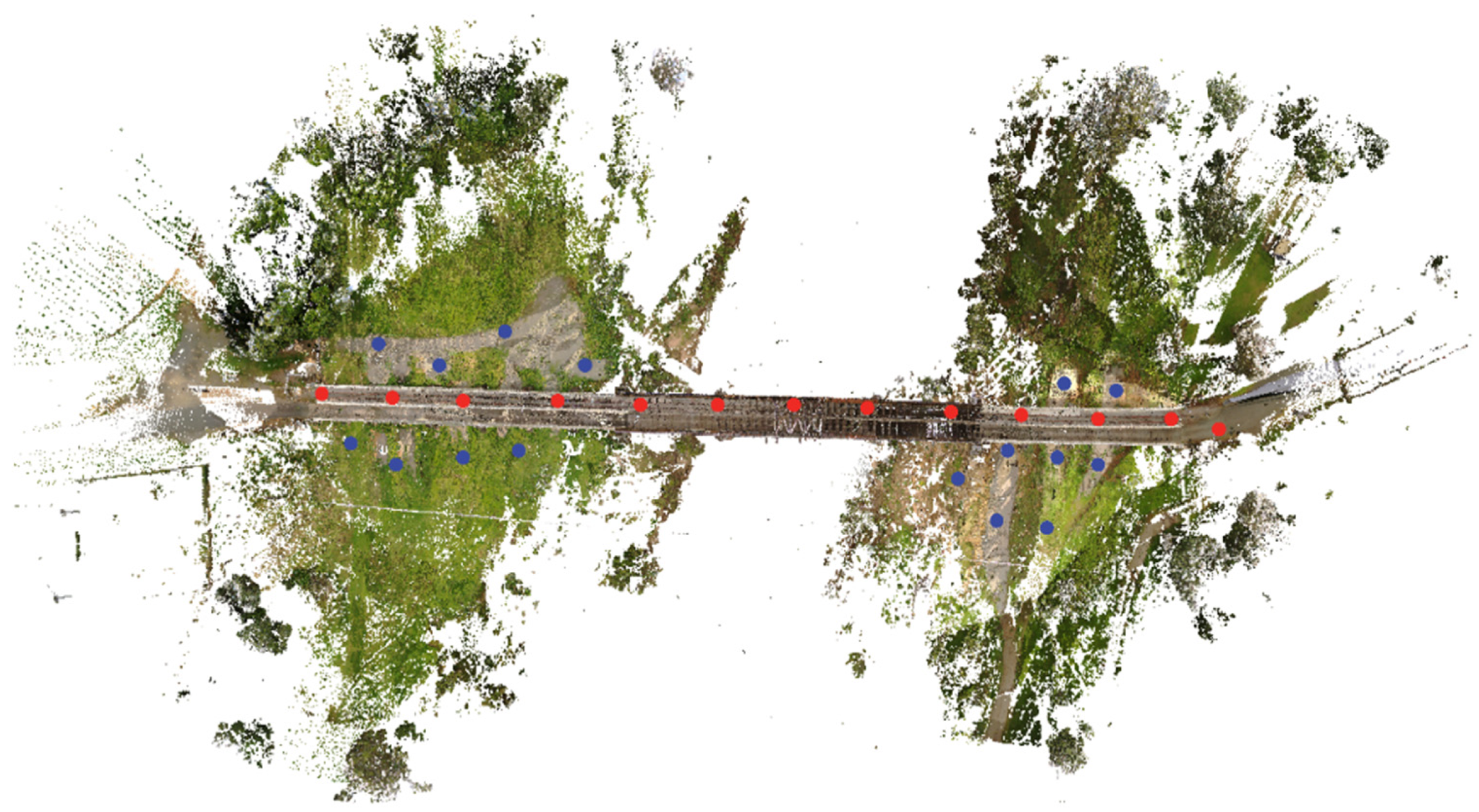
3.3. Point Cloud Data Collection and Noise Removal

A total of 29 scanning points were selected on the Dickabrma Bridge for point cloud collection (Figure 4), resulting in 29 point clouds under independent coordinate systems. During the scanning process, the Faro S70’s built-in GPS, inclinometer, compass, and altimeter recorded the corresponding scanning position information. The data, harnessed from the built-in sensors of the FS70, can be employed for the coarse registration between raw point clouds. The purpose of this process is to provide these point clouds, initially existing in independent coordinate systems, with relatively good initial positioning within a unified coordinate system. Ultimately, we duplicate the initially configured point cloud data into two sets. The first set (Scenario 1) is left without any subsequent processing (Figure 5a). For the second set (Scenario 2), based on the original data, non-bridge components, such as residual images of flowers, trees, and pedestrians, are identified and eliminated as noise points (Figure 5b). Throughout the entire process of point cloud processing, no subsampling operations are involved to prevent the introduction of additional experimental variables that could affect the reliability of the final results.

3.4. Registration Strategies Used in Experiment

In this experiment, a total of six different point cloud registration strategies or algorithms were compared. These strategies are primarily used for fine registration and include point-to-point ICP (POICP), point-to-plane ICP (PLICP), colored registration combined with P2PL (CICP), robust kernels with Iterative Closest Point (KICP), global registration in conjunction with P2PL (GRICP), and fast global registration with P2PL (FGRICP). All algorithms were primarily executed using Python 3.8.4, utilizing libraries such as Open3D and Numpy.

3.4.1. Point-to-Point ICP (POICP)

P2PO is the most fundamental ICP algorithm. Its objective is to finely register two adjacent point clouds—source and target—that are initially in relatively good alignment. This alignment is achieved by iteratively finding correspondence sets and updating transformation matrix T to minimize an objective function [35,57]. This process is defined over three main steps.

The first step involves transforming the position of the source point cloud to the expected position. This transformation is subject to different conditions. If the two adjacent point clouds are already well-placed, meaning they are substantially overlapping, the transformation matrix adopts the identity matrix T₀. However, if the two adjacent point clouds are relatively distant, an initial coarse registration is required to attain the initial transformation matrix T₁. In this study, as each point cloud is already well-positioned due to the FS70 built-in sensor, we adopt the approach of using the identity matrix T₀:

$$T_0=\left[\begin{array}{cccc}1& 0& 0& 0\\ 0& 1& 0& 0\\ 0& 0& 1& 0\\ 0& 0& 0& 1\end{array}\right]$$

(1)

The second step is to perform the nearest point search within a certain range in the target point cloud, forming initial point pairs. The search range used in this experiment is 0.02 m. This step involves finding the correspondence set K = {(p_i, q_i)} from the target point cloud P and the source point cloud Q:

$$p_i\in P=\left\{p_1,p_2,\dots ,p_n\right\}$$

(2)

$$\begin{array}{c}{q}_i\in Q=\left\{q_1,q_2,\dots ,q_n\right\}\end{array}$$

(3)

$$\begin{array}{c}\left(p_i,q_i\right)\in K=\left\{\left(p_1,q_1\right),\left(p_2,q_2\right),\left(p_3,q_3\right),\dots ,\left(p_n,q_n\right)\right\}\end{array}$$

(4)

After forming the initial point pairs, the algorithm enters the phase of minimizing an objective function E(T):

$$E\left(T\right)=\sum _{i=1}^n{\left|\left|p_i-T{q}_i\right|\right|}^2$$

(5)

This objective function represents the sum of the squared differences between each pair of corresponding points (p_i, q_i), where pi is a point in the target point cloud and Tq_i is a point in the transformed source point cloud. The transformation matrix T is then updated by finding the T that minimizes E(T).

3.4.2. Point-to-Plane ICP (PLICP)

P2PL is also one of the fundamental algorithms in ICP. The principle of registration in P2PL is very similar to that in P2PO. However, P2PL, while considering the spatial relationship of point pairs as P2PO does, also takes into account the influence of the normal vector of the points [35]. The calculation of a normal vector for a point within a point cloud is typically a two-step process. The first step involves conducting a nearest neighbor search for a specific point in the point cloud. The second step involves determining the normal vector for that point, which is normally achieved either through methods such as principal component analysis (PCA) or plane fitting techniques. In the context of this research, we derive the normal vector and compute the objective function by leveraging the functionalities provided by the ‘TransformationEstimationPointToPlane’ method within the Open3D library. This class offers efficient implementations for calculating the normal vectors for each point in a point cloud and for formulating the objective function. The objective function can be expressed as follows:

$$E\left(T\right)=\sum _{i=1}^n{\left((p_i-T{q}_i)·n_{p_i}\right)}^2$$

(6)

where E(T) is the objective function that we aim to minimize. It represents the sum of squared distances from each point in the transformed source point cloud (q_i) to the corresponding point in the target point cloud (p_i), weighted by the dot product with the normal of the source point. T is the transformation matrix that we are solving for. It represents the rotation and translation that best aligns the q_i to the target p_i. p_i denotes a point in the target point cloud P. q_i represents a corresponding point in the source point cloud Q, transformed by T. n_pi is the normal vector at point p_i in the target point cloud.

3.4.3. Colored ICP (CICP)

Colored ICP is a variant based on the vanilla ICP (often referred to as POICP or PLICP). This method was proposed by Park at the ICCV in 2017 [58]. Unlike the vanilla ICP, which only considers the optimization of the geometric objective, Colored ICP additionally incorporates the optimization of color differences into the objective function. As a result, its objective function is a composite of two different objective functions, each with its own weight:

$$\begin{array}{c}E\left(T\right)=\left(1-\delta \right)E_C\left(T\right)+\delta E_G\left(T\right)\end{array}$$

(7)

where T denotes the transformation matrix that we aim to estimate. E_C and E_G symbolize the photometric and geometric components, respectively. The weight factor δ, which lies in the range of (0, 1), is established based on empirical data.

The geometric term E_G is, in fact, consistent with the objective function of the vanilla ICP, and the objective function based on PLICP is adopted in this paper. (Please see Equation (6)).

The color term E_C quantifies the disparity in color between point q_i, represented as C(q_i), and the color of its projected counterpart on the tangent plane of point p_i:

$$\begin{array}{c}{E}_C\left(T\right)={\displaystyle \sum _{i=1}^n}{\left(C_{p_i}\left(f\left(T{q}_i\right)\right)-C\left(q_i\right)\right)}^2\end{array}$$

(8)

where, Tq_i represents the i-th indexed point in the source point cloud after transformation, and f (.) is a projection function that maps Tq_i to the tangent plane of the i-th indexed point (p_i) in the target point cloud. C_pi (.) is a continuously varying function based on the color of p_i, used to quantify the color of the projected point of q_i on the tangent plane of p_i.

3.4.4. Robust Kernels ICP (KICP)

KICP, which incorporates the use of Robust Kernels on top of the vanilla ICP, is designed primarily to mitigate the impact of outliers on the final results [59]. Initially, the Robust Kernels function ($\rho$ (.)) generates a weight, denoted as w_i, based on the squared residuals between the point pairs (p_i, q_i). This weight w_i will be smaller when the squared residuals between p_i and q_i are larger:

$$\begin{array}{c}{w}_i=\frac{1}{\left(p_i-T{q}_i\right)·n_{p_i}}{\rho }^{\prime }\left((p_i-T{q}_i)·n_{p_i}\right)\end{array}$$

(9)

where q_i represents the source point in the point pair, p_i represents the corresponding target point in the point pair, T is the transformation matrix, n_pi represents the norm used and calculated based on p_i, and ρ′ is the derivative of the Robust Kernel function applied to the squared residual between p_i and q_i.

With these weights (w_i), the objective function of KICP can be expressed as:

$$\begin{array}{c}E\left(T\right)={\displaystyle \sum _{i=1}^n}{w}_i{\left((p_i-T{q}_i)·n_{p_i}\right)}^2\end{array}$$

(10)

In this objective function, the summation extends over all point pairs, each contributing a term that is the squared residual weighted by the corresponding w_i. This ensures that the well-matched point pairs (i.e., pairs with smaller residuals) have a more substantial influence on the final transformation estimate, while the outliers (i.e., pairs with larger residuals) have their influence substantially diminished. This mechanism underlies the robustness of the KICP algorithm.

By iteratively minimizing this weighted objective function using techniques like Gauss-Newton, we can estimate the optimal transformation matrix that best aligns the source point cloud to the target. This results in an enhanced point-to-plane ICP algorithm that is robust to outliers and can lead to more accurate point cloud registration.

3.4.5. Global Registration + ICP (GRICP)

The Iterative Closest Point (ICP) algorithm and its variants belong to the category of fine registration techniques, which implies the necessity for a relatively decent initial position to establish point correspondences for alignment. However, in many scenarios, even after processing with coarse registration-related methods, this decent initial position is still far from ideal. Global registration algorithms are designed to automatically optimize this initial position, facilitating the ICP algorithm to generate a more accurate set of point correspondences at the very beginning of its operation. The procedure for global registration predominantly unfolds in two phases. During the initial phase, the Fast Point Feature Histogram (FPFH) descriptors are computed for each individual point in both the source and target point clouds [60]. Subsequently, the Random Sample Consensus (RANSAC) method [61] was applied for global registration. With each RANSAC iteration, a subset of points is randomly picked from the source point cloud. By querying the nearest neighbor in the 33-dimensional FPFH feature space, we locate the corresponding points in the target point cloud.

In the subsequent phase, rapid pruning algorithms are employed early on to swiftly discard mismatches during the pruning step. Open3D library offers various pruning algorithms:

• ‘CorrespondenceCheckerBasedOnDistance’ confirms whether the distances between aligned point clouds are within a specific threshold.
• ‘CorrespondenceCheckerBasedOnEdgeLength’ assesses whether the lengths of two arbitrary edges (lines formed by two points), derived individually from source and target correspondences, exhibit similarity. This check verifies the conditions ||source edge length|| > 0.9 * ||target edge length|| and ||target edge length|| > 0.9 * ||source edge length||.
• ‘CorrespondenceCheckerBasedOnNormal’ evaluates the affinity of vertex normal for any given correspondences. This is performed by computing the dot product of two normal vectors, using a radian value as the threshold.

Only those matches that successfully pass through the pruning phase are leveraged to compute a transformation. This transformation is subsequently validated across the entirety of the point cloud. The crucial function deployed in this procedure is ‘registration_ransac_based_on_feature_matching’. The most crucial hyperparameter for this function is ‘the RANSACConvergenceCriteria’, which stipulates the maximum iterations for RANSAC and the confidence probability. The higher these parameters, the greater the accuracy of the results, albeit at the cost of a longer algorithm execution time.

Upon the completion of global registration, we are able to optimize an initial transformation matrix, denoted as T₁. The source point cloud, when transformed by this initial matrix, can align with the target point cloud at a more precise initial position. This alignment serves as the basis for executing the ICP algorithm.

3.4.6. Fast Global Registration + ICP (FGRICP)

In the process of global registration, RANSAC represents an iterative model estimation method, involving a substantial number of point pair proposals and evaluations. This constitutes a highly time-consuming algorithmic process. Fast Global Registration, however, is an alternative method for global registration, outperforming the RANSAC-based approach in terms of computational efficiency. This method was introduced by Qian-Yi Zhou in his 2016 paper titled Fast Global Registration [62].

The crux of the Fast Global Registration lies in the optimization of linear process weights to identify the best correspondences, thereby achieving model registration. In contrast to RANSAC, this method eliminates the need for copious model proposals and evaluations, resulting in significantly enhanced computational efficiency.

The Fast Global Registration algorithm proceeds as follows:

• Feature Extraction and Matching: Initially, features are extracted from the two adjacent point clouds that need to be registered. Based on these features, matching is performed to identify potential point pairs. In the experiment, the feature is the same as the global registration, which is FPFH.
• Graph Model Construction: Using the matched point pairs, a graph model is constructed where each edge represents a point pair.
• Linear Process Weight Optimization: The next step involves the optimization of the linear process weights to determine the significance of each point pair. This step is central to the Fast Global Registration algorithm and the reason for its efficient performance. The aim of optimization is to achieve as much consistency as possible in the model after registration.
• Iterative Optimization: Iterative optimization continues until the model converges or a predetermined number of iterations are reached.
• Final Registration Result: Finally, the optimized linear process weights are used to obtain the final registration result.

Upon completion of the fast global registration, a similar effect to that of the global registration can be achieved, optimizing the initial positions of the source and target point clouds. Subsequently, superior precision can be realized through the utilization of the ICP algorithm.

3.5. Registration Error and Time Consumption

In previous studies, it has been substantiated that the quality of point cloud registration can significantly affect the accuracy of the resultant point cloud model [27]. The current research primarily employs two metrics, namely RE and TC, to assess the quality of point cloud registration tasks.

The computation of RE data primarily relies on the transformation matrix T, derived from each registration operation conducted by a specific registration algorithm. Utilizing this transformation matrix T, we can translocate the current source point cloud. Subsequently, the data structure of the target point cloud is optimized based on the kd-tree algorithm. Further, using the nearest-neighbor search method within a 0.02 m range (d), each point in the target point cloud is matched with the closest point in the source point cloud, resulting in pairs. Subsequently, the Euclidean distances for each pair of points are computed, and the median of these distances is selected as the RE value for the current pair of point clouds. The process of calculating TC data predominantly relies on the time function from the time library. Before each execution of the related point cloud registration algorithm, a start time is established. Following the computation of the transformation matrix T using the point cloud registration algorithm, an end time is set. The difference between the end time and the start time allows us to ascertain the time consumption required for the current point cloud registration algorithm to process the given source and target point clouds (Algorithm 1).

Algorithm 1. The pseudocode for the computational procedure of RE and TC

Input: source point cloud Q, target point cloud P, distance threshold d Output: registration error RE, time consumption TC

1: Initialize start time as now () 2: For each registration operation in the specific registration algorithm: 3:     Calculate transformation matrix T 4:     Transform source point cloud Q using T to get Q’ 5: Set end time as now () 6: Calculate TC as the difference between end time and start time 7: Initialize kd-tree based on target point cloud P 8: Initialize pairs as an empty list 9: For each point qi in Q’: 10:     Find the closest point pi in P using kd-tree within range d 11:     Add the pair (pi, qi) to pairs 12: Initialize distances as an empty list 13: For each pair (pi, qi) in pairs: 14:     Calculate the Euclidean distance between pi and qi 15:     Add the distance to distances 16: Calculate RE as the median of distances 17: Return TC, RE

3.6. Significance and Value Analysis

This experiment primarily employs ANOVA (Analysis of Variance) plus Tukey’s HSD test and the Value Engineering Method to, respectively, 1. ascertain whether the differences among various registration methods under the same environmental conditions (with or without noise removal) possess statistical significance, and 2. quantify the value of specific registration algorithms under a particular environment.

ANOVA and Turkey’s HSD test are relatively straightforward statistical analysis methods, the specifics of which can be referred to in Abdi and Williams [63]. Following this, the emphasis of this article is to elaborate on the utilization of the Value Engineering method employed here to quantify the value of each registration strategy under the same environmental conditions.

The first step involves the calculation of the mean RE and TC for the same registration method under the same environmental conditions:

$$Ave(R{E}_d)=\frac{{\sum }_{i=1}^{n}R{E}_{di}}{n}$$

(11)

where Ave (RE_d) denotes the average RE value under the d-th point cloud registration algorithm. RE_di refers to the i-th RE value under the same d-th point cloud registration algorithm.

$$Ave\left(T{C}_d\right)=\frac{{\sum }_{i=1}^{n}T{C}_{di}}{n}$$

(12)

where Ave (TC_d) denotes the average TC value under the d-th point cloud registration algorithm. TC_di refers to the i-th RE value under the same d-th point cloud registration algorithm.

The second step is to normalize the average RE and TC values obtained for each type of registration strategy under the same environmental conditions. This normalization operation scales these values proportionally within the range of (0, 1). The specific calculation method is as follows:

$$Ave{\left(R{E}_d\right)}^{\prime }=\frac{Ave\left(R{E}_d\right)}{{\sum }_{d=1}^{n}Ave\left(R{E}_d\right)}$$

(13)

where Ave (RE_d)′ represents the normalized RE_d, which is calculated by dividing any given RE_d by the sum of all RE_d under the same environmental conditions.

$$Ave{\left(T{C}_d\right)}^{\prime }=\frac{Ave\left(T{C}_d\right)}{{\sum }_{d=1}^{n}Ave\left(T{C}_d\right)}$$

(14)

where Ave (TC_d)’ represents the normalized TC_d, which is calculated by dividing any given TC_d by the sum of all TC_d under the same environmental conditions.

The third step involves a special treatment of Ave (RE_d)′. Each Ave (RE_d)′ calculated under the same environmental conditions for every registration algorithm needs to be subtracted from (1). This is because Ave (RE_d)′ is intended to represent utility value in subsequent computations, where the logic is that the smaller the error, the larger the utility value. Thus, it is necessary to specially handle Ave (RE_d)′ to achieve this effect:

$$Ave{\left(R{E}_d\right)}^{\prime \prime }=\frac{1-Ave{\left(R{E}_d\right)}^{\prime }}{5}$$

(15)

where Ave (RE_d)′′ represents the specially processed Ave (RE_d)′ and, in subsequent calculations, it denotes the utility value of the current registration algorithm.

The final step involves calculating the value of each point cloud registration strategy under the same environmental conditions:

$$\begin{array}{c}{V}_d=\frac{Ave{\left(R{E}_d\right)}^{\prime \prime }}{Ave\left(T{C}_d\right)\prime }\end{array}$$

(16)

where V_d represents the value corresponding to the d-th point cloud registration algorithm under the same environmental conditions.

4. Result

4.1. Scenario 1 (Non-Noise Removal)

In this experiment, the quality of six different point cloud registration strategies was tested under non-noise-removal environmental conditions. Each point cloud registration strategy was applied to 28 pairs of point clouds, resulting in 28 RE data and 28 TC data for each strategy. In total, all registration strategies produced 168 RE data and 168 TC data.

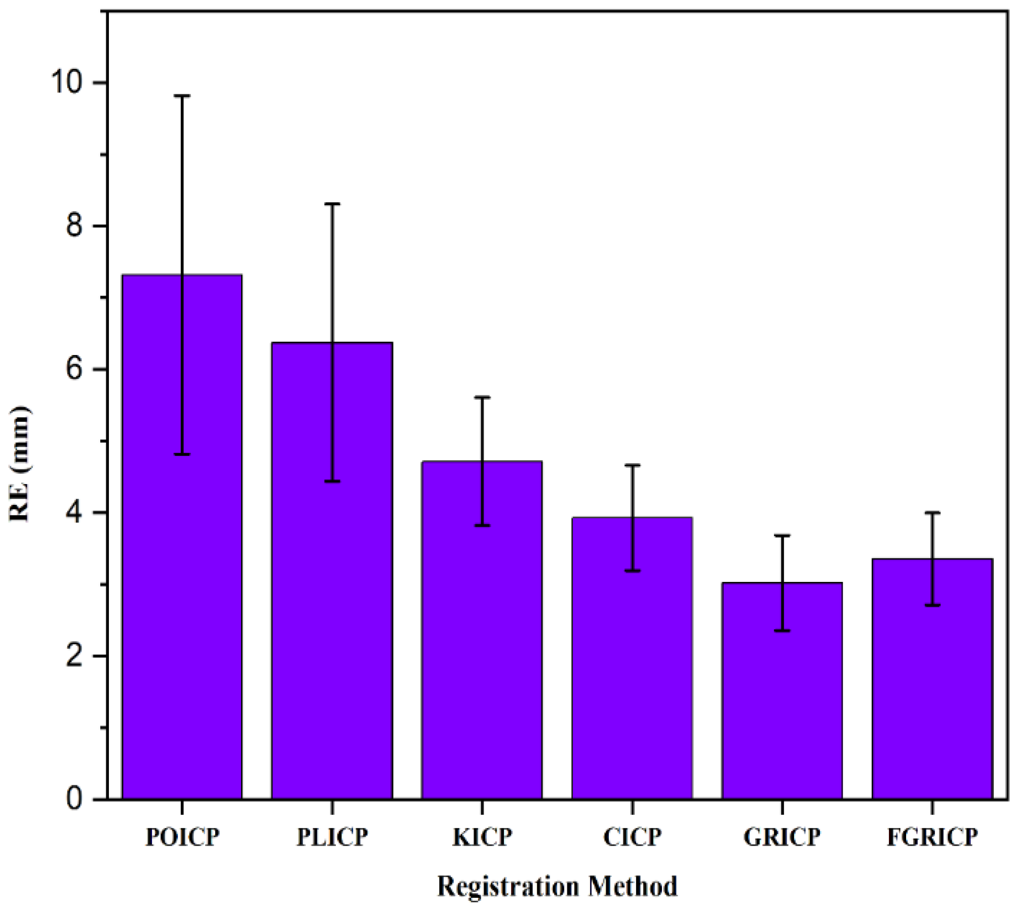
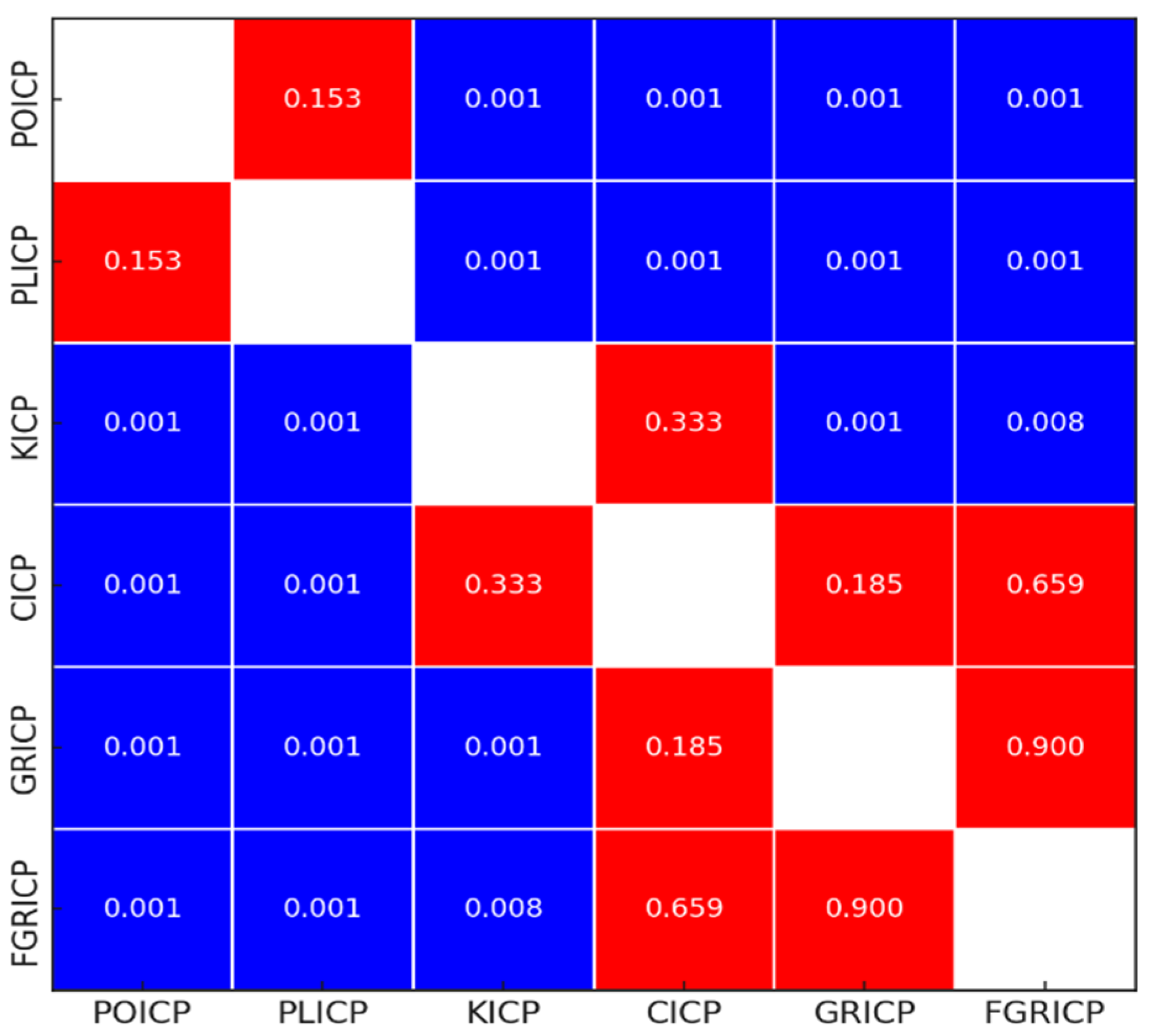
4.1.1. Registration Error

According to the descriptive analysis of these 168 RE data (

Table 1. Descriptive analysis for RE under non-noise removal condition.

Method	Count	Sum	Average	Variance
POICP	28	204.87	7.32	6.49
PLICP	28	178.51	6.38	3.88
KICP	28	131.95	4.71	0.82
CICP	28	108.96	3.93	0.56
GRICP	28	107.97	3.02	0.42
FGRICP	28	117.39	3.36	0.46

), the average error is ranked from largest to smallest as follows: POICP (7.32 mm), PLICP (6.38 mm), KICP (4.71 mm), CICP (3.93 mm), FGRICP (3.36 mm), GRICP (3.02 mm). We found that GRICP has the smallest average RE, indicating the highest precision in registration. Concurrently, the variance of the registration error of the GRICP algorithm is also the smallest, which signifies that this method exhibits excellent stability in performing registration tasks under a non-noise removal environment. Conversely, the POICP algorithm exhibits the highest average RE values as well as the largest variance, implying that the current algorithm has a lower overall accuracy and exhibits instability in its error range (Figure 6).

Based on the results of the ANOVA analysis, we observe a p-value of 0.000 (

Table 2. Summary of ANOVA analysis for RE under non-noise removal condition.

Source of Variation	SS	df	MS	F	p-Value	F Crit
Between Groups	415.51	5	83.10	39.43	0.000	2.27
Within Groups	341.45	162	2.11
Total	756.96	167

Note: SS = Sum of Square; df = Degree of Freedom; MS = Mean Square.

). This denotes that, among the six groups, each employing a distinct point cloud registration algorithm to obtain RE data, there is at least one pair with a significant difference in their means. Further interpretation suggests that the registration method is a meaningful variable under conditions of non-noise removal. In a subsequent analysis utilizing the Tukey HSD method (Figure 7), we find that there is no statistical significance in the comparisons between POICP and PLICP (p = 0.153), KICP and CICP (p = 0.333), CICP and GRICP (p = 0.185), CICP and FGRICP (p = 0.659), and GRICP and FGRICP (p = 0.900). This infers that the point cloud accuracy is very close when these groups are compared individually.

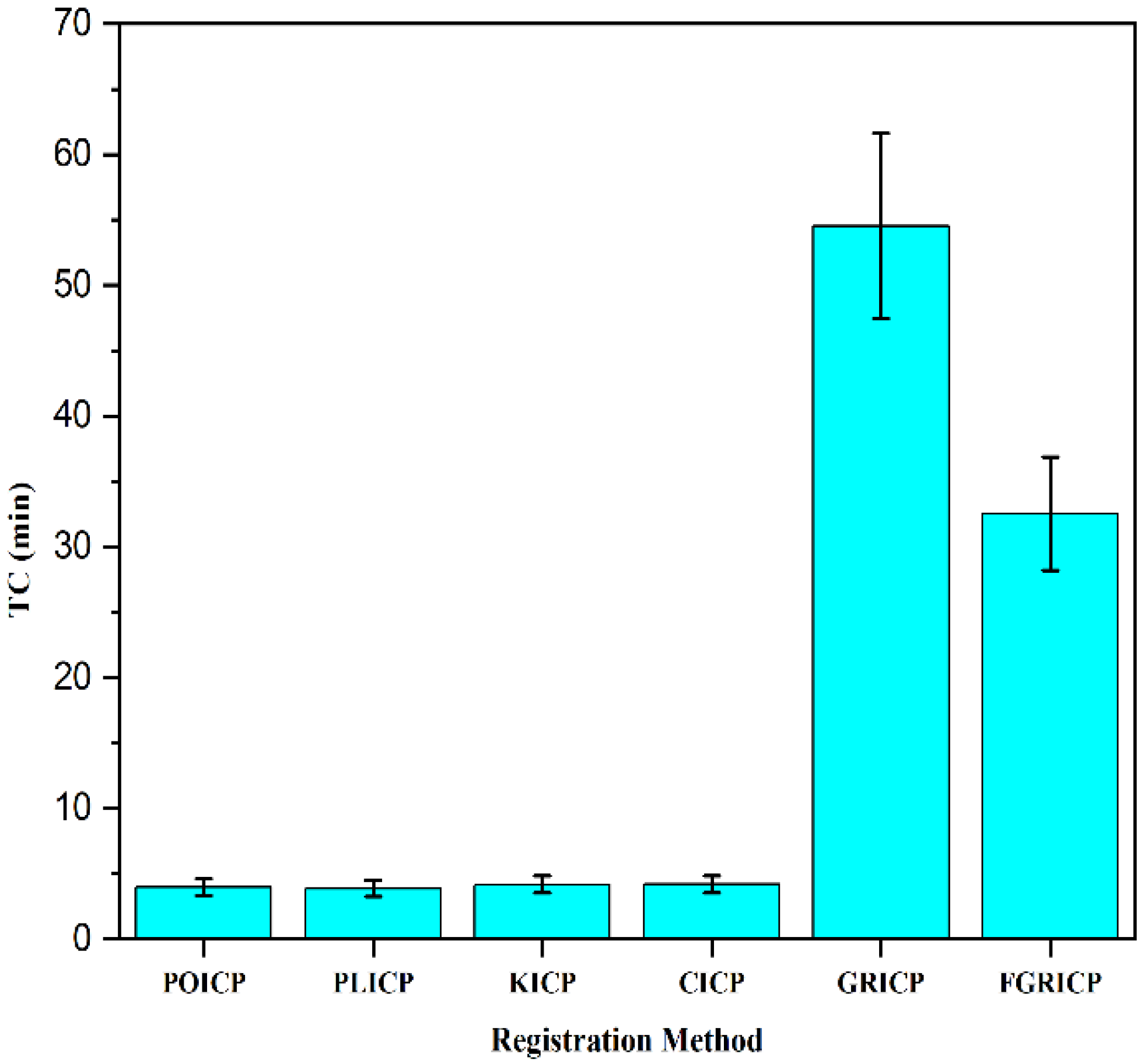
4.1.2. Time Consumption

In an analysis of 168 TC data (

Table 3. Descriptive analysis for TC under non-noise removal condition.

Groups	Count	Sum	Average	Variance
POICP	28	111.48	3.98	0.42
PLICP	28	108.21	3.86	0.37
KICP	28	116.95	4.18	0.43
CICP	28	117.31	4.19	0.45
GRICP	28	1526.87	54.53	51.86
FGRICP	28	910.94	32.53	19.34

), the average TC values, ordered from highest to lowest, are as follows: GRICP (54.53 min), FGRICP (32.53 min), CICP (4.19 min), KICP (4.18 min), POICP (3.98 min), and PLICP (3.86 min). Of these, the PLICP algorithm has the smallest mean value. This implies that, based on the overall sample, the PLICP algorithm can compute the required results in the shortest amount of time. Additionally, it also has the smallest variance, demonstrating a high level of stability in its time consumption. Conversely, GRICP has the highest mean value, indicating a high time cost for running the algorithm and a relatively low level of stability in its execution time (Figure 8).

Based on the ANOVA analysis of the total TC data, I obtained a p-value of 0.000 (

Table 4. Summary of ANOVA analysis for TC under non-noise removal condition.

Source of Variation	SS	df	MS	F	p-Value	F Crit
Between Groups	64,964.54	5	12,992.91	1069.61	0.000	2.27
Within Groups	1967.87	162	12.15
Total	66,932.41	167

Note: SS = Sum of Square; df = Degree of Freedom; MS = Mean Square.

), which indicates that the registration method is a significant influencing factor in the time consumption of point cloud registration. Further, based on the Tukey HSD test for intergroup data analysis (Figure 9), we found that POICP vs. PLICP (p = 0.900), POICP vs. KICP (p = 0.900), POICP vs. CICP (p = 0.900), PLICP vs. KICP (p = 0.900), PLICP vs. CICP (p = 0.900), and KICP vs. CICP (p = 0.900), and there is no significant difference in time consumption for the five groups of registration methods.

4.1.3. Value Comparison

According to the calculations using the value engineering method, we obtained the value scores (V_d) for six different registration methods in a non-noise removal environment (

Table 5. Value comparison between different registration methods under non-noise removal condition.

Registration Method	Ave (REd)′′	Ave (TCd)′	Vd
POICP	0.15	0.04	3.87
PLICP	0.16	0.04	4.16
KICP	0.17	0.04	4.13
CICP	0.17	0.04	4.26
GRICP	0.18	0.53	0.34
FGRICP	0.18	0.32	0.56
Total	1.00	1.00	17.31

). From highest to lowest, they are: CICP (4.26), PLICP (4.16), KICP (4.13), POICP (3.87), FGRICP (0.56), and GRICP (0.34). The final data indicates that the CICP algorithm offers the highest cost-performance ratio, while the GRICP has the lowest (Figure 10).

4.2. Scenario 2 (Noise Removal)

In this experiment, the quality of six different point cloud registration strategies was tested under noise removal conditions. Each point cloud registration strategy was applied to 28 pairs of point clouds, resulting in 28 RE data and 28 TC data for each strategy. In total, all registration strategies produced 168 RE data and 168 TC data.

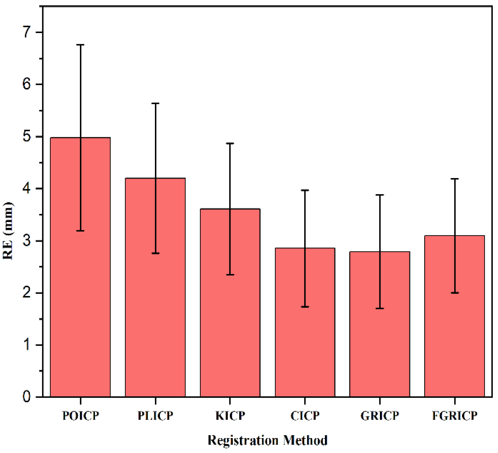
4.2.1. Registration Error

According to the descriptive analysis (

Table 6. Descriptive analysis for RE under noise removal condition.

Method	Count	Sum	Average	Variance
POICP	28	139.34	4.98	3.30
PLICP	28	117.59	4.20	2.14
KICP	28	101.09	3.61	1.64
CICP	28	79.94	2.86	1.30
GRICP	28	78.18	2.79	1.23
FGRICP	28	86.73	3.10	1.24

), the six different point cloud registration methods produce an average point cloud error in a noise-removal environment, ranked from highest to lowest as follows: POICP (4.98 mm), PLICP (4.20 mm), KICP (3.61 mm), FGRICP (3.10 mm), CICP (2.86 mm), and GRICP (2.79 mm). Of these, GRICP remains the algorithm with the highest precision in point cloud registration, and its variance of 1.23 mm also indicates good stability. Conversely, POICP has the lowest precision in point cloud registration and, with a variance of 3.30 mm, it is relatively unstable (Figure 11).

Based on the ANOVA analysis (

Table 7. Summary of ANOVA analysis for RE under noise removal condition.

Source of Variation	SS	df	MS	F	p-Value	F Crit
Between Groups	103.98	5	20.80	11.49	0.000	2.27
Within Groups	293.16	162	1.81
Total	397.14	167

Note: SS = Sum of Square; df = Degree of Freedom; MS = Mean Square.

), a final p-value of 0.000 was obtained, indicating that the registration method remains a statistically significant factor influencing registration error in a noise removal environment. Further analysis through the Tukey HSD test resulted in the following findings (Figure 12): POICP vs. PLICP (p = 0.262), PLICP vs. KICP (p = 0.564), KICP vs. CICP (p = 0.292), KICP vs. GRICP (p = 0.210), KICP vs. FGRICP (0.685), CICP vs. GRICP (p = 0.900), CICP vs. FGRICP (p = 0.900), and GRICP vs. FGRICP (p = 0.900). The p-values of all these eight combinations exceed 0.1, indicating that there is no significant difference in RE produced between the registration methods within these combinations. Apart from these eight combinations, significant differences were displayed when comparing the remaining combinations.

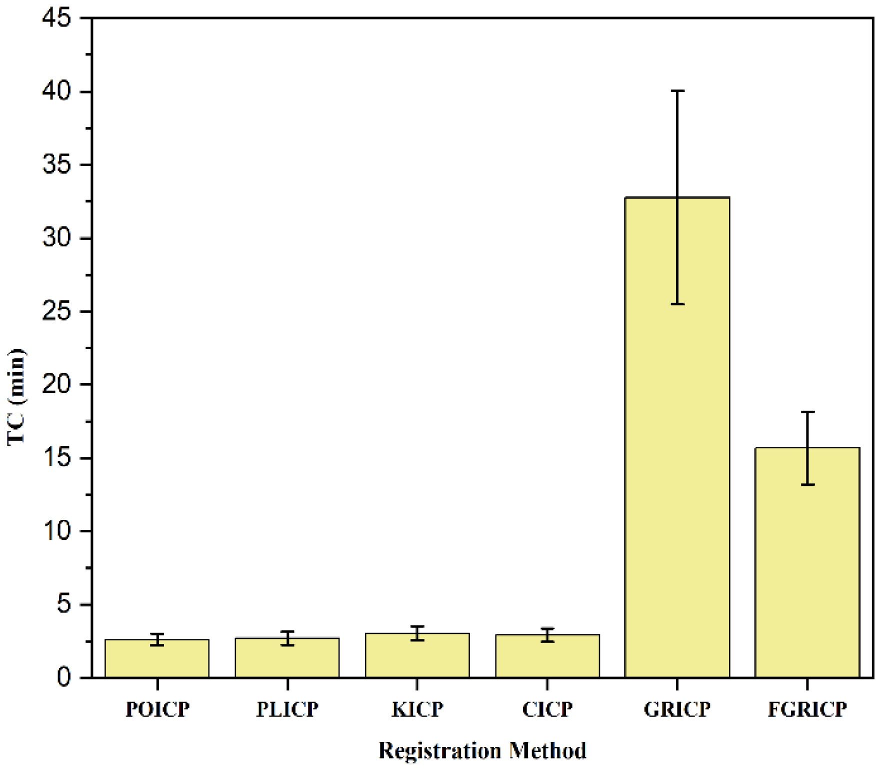
4.2.2. Time Consumption

Based on the descriptive analysis of TC (

Table 8. Descriptive analysis for TC under noise removal condition.

Method	Count	Sum	Average	Variance
POICP	28	73.06	2.61	0.16
PLICP	28	75.51	2.70	0.20
KICP	28	84.84	3.03	0.24
CICP	28	81.23	2.90	0.22
GRICP	28	917.27	32.76	54.91
FGRICP	28	439.09	15.68	6.40

), we can rank the different point cloud registration methods in terms of average time consumption from highest to lowest in a noise-removal environment: GRICP (32.76 min), FGRICP (15.68 min), KICP (3.03 min), CICP (2.90 min), PLICP (2.70 min), and POICP (2.61 min). Among these, POICP has the least runtime and an intra-group variance of only 0.16 min, indicating the stability of this algorithm in terms of time consumption. In contrast, GRICP takes the longest time, with a variance as high as 54.91. This implies that the algorithm’s performance in terms of time consumption is highly unstable, with a large range, making it hard to predict (Figure 13).

Based on the ANOVA analysis (

Table 9. Summary of ANOVA analysis for TC under noise removal condition.

Source of Variation	SS	df	MS	F	p-Value	F Crit
Between Groups	21,201.66	5	4240.33	409.46	0.000	2.27
Within Groups	1677.65	162	10.36
Total	22,879.31	167

Note: SS = Sum of Square; df = Degree of Freedom; MS = Mean Square.

), we obtained a p-value of 0.000, indicating that the registration method has a significant impact on time consumption in a noise-removal environment. Further analysis using the Tukey HSD test (Figure 14) resulted in POICP vs. PLICP (p = 0.900), POICP vs. KICP (p = 0.900), POICP vs. CICP (p = 0.900), PLICP vs. KICP (p = 0.900), PLICP vs. CICP (p = 0.900), and KICP vs. CICP (p = 0.900). A total of five intra-group comparisons of registration methods revealed no significant differences, and significant differences were found in the remaining intra-group comparisons. This result is almost completely consistent with the results obtained in the Noise-removal test.

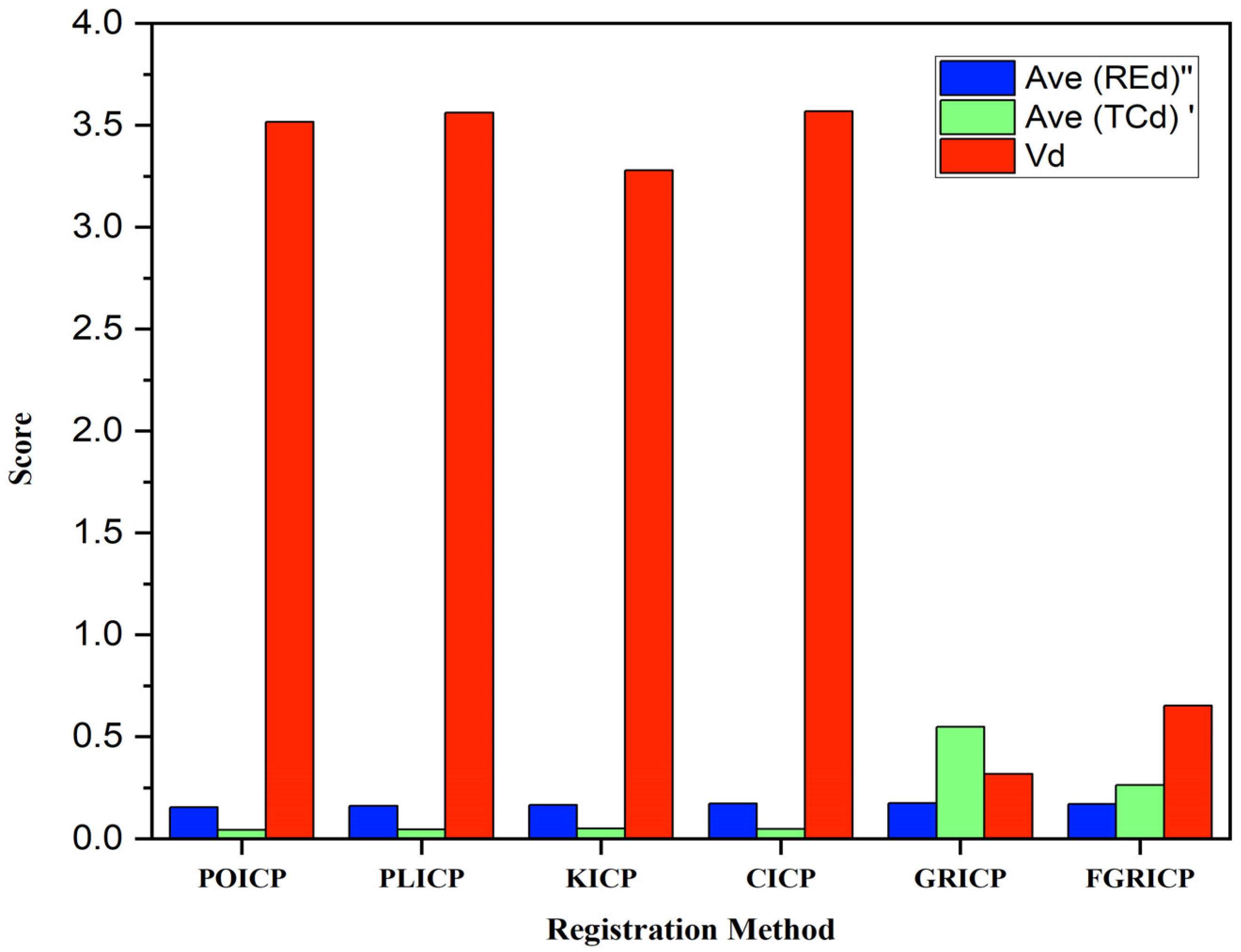
4.2.3. Value Comparison

According to the calculations using the value engineering method (

Table 10. Value comparison between different registration method under noise removal condition.

Registration Method	Ave (REd)′′	Ave (TCd)′	Vd
POICP	0.15	0.04	3.52
PLICP	0.16	0.05	3.56
KICP	0.17	0.05	3.28
CICP	0.17	0.05	3.57
GRICP	0.17	0.55	0.32
FGRICP	0.17	0.26	0.65
Total	1.00	1.00	14.90

), we obtained the value scores (V_d) for six different registration methods in a non-noise removal environment. From highest to lowest, they are: CICP (3.57), PLICP (3.56), POICP (3.52), KICP (3.28), FGRICP (0.65), and GRICP (0.32). The final data indicates that the CICP algorithm offers the highest cost-performance ratio, while the GRICP has the lowest (Figure 15).

4.3. Scenario 1 vs. Scenario 2

In order to investigate the impacts of noise removal and non-noise removal on registration error and time consumption, we conducted t-tests on the same registration method under different conditions. This was performed to ascertain whether varying environments would result in significant effects.

Based on the t-test analysis for RE under the same registration method under different conditions (

Table 11. The result of T-test for RE between noise removal and non-noise removal condition.

Method	t-Value	p-Value	Average RE (Non-Noise Removal)	Average RE (Noise Removal)
POICP	3.96	0.000	7.32	4.98
PLICP	4.69	0.000	6.38	4.20
KICP	3.71	0.001	4.71	3.61
CICP	4.16	0.000	3.93	2.86
GRICP	0.93	0.359	3.02	2.79
FGRICP	1.06	0.295	3.36	3.10

), we obtained the p-values for the same registration method under different conditions, which were respectively: POICP (0.000), PLICP (0.000), KICP (0.001), CICP (0.000), GRICP (0.295), and FGRICP (0.359). Among these, with the exception of GRICP and FGRICP, all other algorithms exhibited significant differences between the conditions of noise removal and non-noise removal. This suggests that, in most cases, noise removal serves as a significant influencing factor on registration error, and it can help reduce the registration error and enhance registration accuracy.

According to the t-test analysis for TC under the same registration method for different conditions (

Table 12. The result of t-test for TC between noise removal and non-noise removal condition.

Method	t-Value	p-Value	Average TC (Non-Noise Removal)	Average TC (Noise Removal)
POICP	9.46	0.000	3.98	2.61
PLICP	8.15	0.000	3.86	2.70
KICP	7.39	0.000	4.18	3.03
CICP	8.32	0.000	4.19	2.90
GRICP	11.15	0.000	54.53	32.76
FGRICP	17.58	0.000	32.53	15.68

), we obtained the p-values for the same registration method under different conditions, which were respectively: POICP (0.000), PLICP (0.000), KICP (0.001), CICP (0.000), GRICP (0.000), and FGRICP (0.000). Among these, all point cloud registration algorithms demonstrated significant differences between the conditions of noise removal and non-noise removal. This indicates that noise removal is a universally significant influencing factor on time consumption, and it can very effectively reduce time spent, greatly enhancing operational efficiency.

5. Discussion

5.1. Key Findings

The following encapsulates the key findings from our experiment:

• In conditions without noise removal, the average RE for six different point cloud registration methods, listed from highest to lowest, are as follows: POICP (7.32 mm), PLICP (6.38 mm), KICP (4.71 mm), CICP (3.93 mm), FGRICP (3.36 mm), GRICP (3.02 mm). When operating under conditions with noise removal, the average Registration Error (RE) values from highest to lowest are: POICP (4.98 mm), PLICP (4.20 mm), KICP (3.61 mm), FGRICP (3.10 mm), CICP (2.86 mm), and GRICP (2.79 mm).
• Under conditions without noise removal, the TC for six different point cloud registration methods, listed from highest to lowest, are as follows: GRICP (54.53 min), FGRICP (32.53 min), CICP (4.19 min), KICP (4.18 min), POICP (3.98 min), and PLICP (3.86 min). When operating under conditions with noise removal, the Time Consumption (TC) values, from highest to lowest, are: GRICP (32.76 min), FGRICP (15.68 min), KICP (3.03 min), CICP (2.90 min), PLICP (2.70 min), and POICP (2.61 min).
• In the non-noise removal condition, the score of value engineering for CICP was 4.26, while under the noise removal condition, it scored 3.57. In both conditions, CICP achieved the highest score. This suggests that CICP is the most cost-effective point cloud registration algorithm in this experiment. Its overall performance is outstanding, with average registration errors of 3.93 mm (non-noise removal) and 2.86 mm (noise removal), respectively. The average time consumption is 4.19 min (non-noise removal) and 2.90 min (noise removal), respectively.
• In the analysis of value engineering, GRICP scored 0.34 and 0.32 under non-noise removal and noise removal conditions, respectively. These are the lowest scores under both conditions, suggesting a relatively low cost-effectiveness. Although when solely comparing the registration error, its averages of 3.02 mm (non-noise removal) and 2.79 mm (noise removal) are among the best in their respective groups, the time consumption is extremely long, at 54.53 min (non-noise removal) and 32.76 min (noise removal), respectively.
• Noise removal can significantly enhance registration accuracy and reduce computational time for the majority of point cloud registration algorithms. Among the six algorithms involved in this study, the average reduction in registration error (RE) was 1.20 mm, and the average reduction in time consumption (TC) was 7.27 min under the noise removal condition compared to the non-noise removal condition. Specifically, for the POICP algorithm, the RE and TC were reduced by 32% and 34%, respectively, after noise removal. For PLICP, there was a reduction of 34% in RE and 30% in TC. KICP showed a decrease of 23% in RE and 28% in TC, CICP demonstrated a 27% and 31% decline in RE and TC respectively, GRICP witnessed a reduction of 8% in RE and 40% in TC, and for FGRICP, the RE and TC decreased by 8% and 52%, respectively, after noise removal.

5.2. Future Development Trend

In this study, under the context of building data related to bridging structures, we investigated six different mainstream point cloud registration methods and the impact of noise removal on registration quality. Among them, CICP achieved the best overall score, indicating the highest cost-effectiveness. Unlike other algorithms, CICP incorporates color as an additional dimension in its calculations. This might be a significant reason why it can achieve relatively high accuracy within a reasonable timeframe. However, if high-resolution cameras are not used during point cloud collection or if color information cannot be acquired, this may pose certain limitations to this method. KICP builds upon the traditional ICP by utilizing kernel functions, but when it comes to bridging construction environments, its performance does not exhibit a notably better improvement compared to traditional ICP, like POICP and PLICP. Although the GRICP and FGRICP algorithms underperformed in the aspect of value engineering, they exhibited outstanding performance in registration error metrics under both non-noise removal and noise removal conditions. This can primarily be attributed to these two algorithms conducting more global registration at the initial stage compared to other ICP variants. This puts the ICP algorithm in a comparatively optimal initial state, suggesting that a better starting position contributes to greater accuracy in point pair formation by the ICP. Hence, we can infer that a high-quality initial point pair collection can significantly enhance registration accuracy.

The trend for future point cloud registration methods necessitates continuous improvement in the accuracy of point pair formation. At present, most algorithms depend on the range search for nearest points or certain feature computations, such as FPFH, 3DSC and SHOT, among others. The former has relatively lower accuracy and requires an excellent initial position to circumvent falling into local optima. In contrast, the latter, although potentially more precise, incurs high computational costs in resources and time, impeding the development of iterative algorithms.

The author proposes the exploration of a deep learning framework grounded in big data, which learns point cloud registration features to create pairs. The potential of this approach resides in its capacity to reconcile accuracy with computational costs, two often conflicting aspects in this field. Theoretically, by employing a data-driven approach, the system could generalize and predict more accurate point pairs, thus potentially improving registration performance.

Nonetheless, the transition towards this approach introduces a new set of challenges that researchers need to confront. Firstly, implementing a deep learning model for this task could involve high learning costs. This is due to the computationally expensive nature of these models, especially when dealing with extensive datasets, as well as the expertise required to design and optimize such models.

Secondly, the scarcity of high-quality datasets for training the model poses a significant challenge. While there are public datasets available for point cloud registration, the extent and variety of these datasets might not be sufficient for training a robust deep learning model that can generalize well to different environments and scenarios.

Lastly, the complexities involved in designing an appropriate deep learning architecture and the difficulties in training such a model cannot be overlooked. This process requires careful consideration of various factors such as the choice of layers, the use of activation functions, the optimization of loss functions, and others. The training of the model also needs to be properly managed to avoid issues such as overfitting or underfitting.

5.3. Experimental Statement and Limitation

• In this study, all point cloud data were not subsampled during the calculation of RE and TC. The only exception was when calculating the FPFH for GRICP and FGRICP, where subsampling was applied due to the extensive duration of the global registration process associated with these methods.
• The measure of TC in this study only encompasses the period from the commencement of the algorithm to the determination and transformation of the source point cloud via the transformation matrix T. It does not include the subsequent time for Registration Error (RE) calculation. The calculation of RE involves traversing all newly formed point pairs within the RE algorithm and computing the Euclidean distance, a process that is notably time-consuming.
• The primary objective of the RE and TC metrics in this paper is to aid in evaluating the significance of the registration method and noise removal as influential factors, as well as assisting in assessing the value of each registration method. The results of RE and TC in this study should only be used as a reference under similar environmental conditions to those detailed in this paper, and where no point cloud subsampling is performed. This is because the calculation of RE in this study is highly sensitive to environmental factors and point cloud subsampling. In particular, subsampling that increases the intervals between point clouds can have a substantial impact on the results.
• The RE calculation method utilized in this study has certain limitations, including its high sensitivity to subsampling, low robustness, and a propensity for local optimal solutions due to the range search for the nearest points. To address these limitations, the author proposes an alternative approach for future researchers. Specifically, the use of markers during scanning could provide a more accurate method for evaluating registration accuracy. By placing markers within the source and target point clouds, these known points can serve as references. Consequently, the Euclidean distance between these markers can be computed as the RE, providing a more accurate reflection of registration accuracy.

6. Conclusions

The main purpose of this study is to investigate the significant impact of registration methods and noise removal on the registration quality of point clouds. The experimental design primarily employed the method of controlled variables to explore the significant influence of registration methods under the same environmental conditions and identical noise removal settings. Additionally, the effect of noise removal was studied by comparing the same registration method under different noise removal conditions. To facilitate the exploration of influencing factors and quantify registration quality, the study utilized RE and TC as quantitative indicators. The final results indicate that the CICP algorithm is the best-performing point cloud registration method in bridging construction environments. Under non-noise removal conditions and noise-removal conditions, its average RE can reach 3.93 mm and 2.86 mm, respectively, while the TC can achieve 4.19 min and 2.86 min, respectively. On the other hand, GRICP stands out as the algorithm with the highest average point cloud registration accuracy in bridging construction contexts, attaining an RE of 3.02 mm under non-noise removal and 2.79 mm under noise removal conditions. However, this algorithm is also the most time-consuming, with time expenditures averaging 54.53 min and 32.76 min under the respective conditions. A marked increase in accuracy and a reduction in processing time were observed for most algorithms following noise removal. Specifically, the POICP algorithm experienced a 32% reduction in RE and a 34% decline in TC after noise removal. Similarly, PLICP observed a 34% and 30% reduction in RE and TC, respectively. KICP showcased a decline of 23% in RE and 28% in TC, CICP manifested a 27% and 31% drop in RE and TC, respectively, GRICP observed an 8% reduction in RE and a 40% decline in TC, and for FGRICP, RE and TC decreased by 8% and 52%, respectively, subsequent to noise removal.

References

1. Aydin, C.C. Designing building façades for the urban rebuilt environment with integration of digital close-range photogrammetry and geographical information systems. Autom. Constr. 2014, 43, 38–48. [Google Scholar] [CrossRef]
2. Bouzas, Ó.; Cabaleiro, M.; Conde, B.; Cruz, Y.; Riveiro, B. Structural health control of historical steel structures using HBIM. Autom. Constr. 2022, 140, 104308. [Google Scholar] [CrossRef]
3. Valero, E.; Bosché, F.; Forster, A. Automatic segmentation of 3D point clouds of rubble masonry walls, and its application to building surveying, repair and maintenance. Autom. Constr. 2018, 96, 29–39. [Google Scholar] [CrossRef]
4. Ursini, A.; Grazzini, A.; Matrone, F.; Zerbinatti, M. From scan-to-BIM to a structural finite elements model of built heritage for dynamic simulation. Autom. Constr. 2022, 142, 104518. [Google Scholar] [CrossRef]
5. Kong, X.; Hucks, R.G. Preserving our heritage: A photogrammetry-based digital twin framework for monitoring deteriorations of historic structures. Autom. Constr. 2023, 152, 104928. [Google Scholar] [CrossRef]
6. Wang, Q.; Kim, M.-K. Applications of 3D point cloud data in the construction industry: A fifteen-year review from 2004 to 2018. Adv. Eng. Inform. 2019, 39, 306–319. [Google Scholar] [CrossRef]
7. Tang, P.; Huber, D.; Akinci, B.; Lipman, R.; Lytle, A. Automatic reconstruction of as-built building information models from laser-scanned point clouds: A review of related techniques. Autom. Constr. 2010, 19, 829–843. [Google Scholar] [CrossRef]
8. Moon, D.; Chung, S.; Kwon, S.; Seo, J.; Shin, J. Comparison and utilization of point cloud generated from photogrammetry and laser scanning: 3D world model for smart heavy equipment planning. Autom. Constr. 2019, 98, 322–331. [Google Scholar] [CrossRef]
9. Page, C.; Sirguey, P.; Hemi, R.; Ferrè, G.; Simonetto, E.; Charlet, C.; Houvet, D. Terrestrial Laser Scanning for the Documentation of Heritage Tunnels: An Error Analysis. In Proceedings of the FIG Working Week, Helsinki, Finland, 29 May–2 June 2017. [Google Scholar]
10. Zhu, Z.; Brilakis, I. Comparison of optical sensor-based spatial data collection techniques for civil infrastructure modeling. J. Comput. Civ. Eng. 2009, 23, 170–177. [Google Scholar] [CrossRef]
11. Aryan, A.; Bosché, F.; Tang, P. Planning for terrestrial laser scanning in construction: A review. Autom. Constr. 2021, 125, 103551. [Google Scholar] [CrossRef]
12. Son, H.; Kim, C.; Turkan, Y. Scan-to-BIM-an overview of the current state of the art and a look ahead. In Proceedings of the ISARC—The International Symposium on Automation and Robotics in Construction, Oulu, Finland, 15–18 June 2015; Volume 32, p. 1. [Google Scholar]
13. Xiong, X.; Adan, A.; Akinci, B.; Huber, D. Automatic creation of semantically rich 3D building models from laser scanner data. Autom. Constr. 2013, 31, 325–337. [Google Scholar] [CrossRef]
14. Haala, N.; Peter, M.; Kremer, J.; Hunter, G. Mobile LiDAR mapping for 3D point cloud collection in urban areas—A performance test. Int. Arch. Photogramm. Remote Sens. Spat. Inf. Sci. 2008, 37, 1119–1127. [Google Scholar]
15. Puente, I.; González-Jorge, H.; Martínez-Sánchez, J.; Arias, P. Review of mobile mapping and surveying technologies. Measurement 2013, 46, 2127–2145. [Google Scholar] [CrossRef]
16. Eker, R. Comparative use of PPK-integrated close-range terrestrial photogrammetry and a handheld mobile laser scanner in the measurement of forest road surface deformation. Measurement 2023, 206, 112322. [Google Scholar] [CrossRef]
17. Williams, K.; Olsen, M.J.; Roe, G.V.; Glennie, C. Synthesis of transportation applications of mobile LiDAR. Remote Sens. 2013, 5, 4652–4692. [Google Scholar] [CrossRef]
18. Thomson, C.; Apostolopoulos, G.; Backes, D.; Boehm, J. Mobile laser scanning for indoor modelling. ISPRS Ann. Photogramm. Remote Sens. Spat. Inf. Sci. 2013, 2, 289–293. [Google Scholar] [CrossRef]
19. Chen, C.; Tang, L.; Hancock, C.M.; Zhang, P. Development of low-cost mobile laser scanning for 3D construction indoor mapping by using inertial measurement unit, ultra-wide band and 2D laser scanner. Eng. Constr. Archit. Manag. 2019, 26, 1367–1386. [Google Scholar] [CrossRef]
20. Harris, C.; Stephens, M. A combined corner and edge detector. In Proceedings of the Alvey Vision Conference, Manchester, UK, 31 August–2 September 1988; Volume 15, pp. 10–5244. [Google Scholar]
21. Lowe, D.G. Object recognition from local scale-invariant features. In Proceedings of the Seventh IEEE International Conference on Computer Vision, Kerkyra, Greece, 20–27 September 1999; Volume 2, pp. 1150–1157. [Google Scholar]
22. Bay, H.; Tuytelaars, T.; Van Gool, L. Surf: Speeded up robust features. Lect. Notes Comput. Sci. 2006, 3951, 404–417. [Google Scholar]
23. Nouwakpo, S.K.; Weltz, M.A.; McGwire, K. Assessing the performance of structure-from-motion photogrammetry and terrestrial LiDAR for reconstructing soil surface microtopography of naturally vegetated plots. Earth Surf. Process. Landf. 2016, 41, 308–322. [Google Scholar] [CrossRef]
24. Kim, M.-C.; Yoon, H.-J. A study on utilization 3D shape pointcloud without GCPs using UAV images. J. Korea Acad.-Ind. Coop. Soc. 2018, 19, 97–104. [Google Scholar]
25. Zhao, L.; Zhang, H.; Mbachu, J. Multi-Sensor Data Fusion for 3D Reconstruction of Complex Structures: A Case Study on a Real High Formwork Project. Remote Sens. 2023, 15, 1264. [Google Scholar] [CrossRef]
26. Będkowski, J. Benchmark of multi-view Terrestrial Laser Scanning Point Cloud data registration algorithms. Measurement 2023, 219, 113199. [Google Scholar] [CrossRef]
27. Zhu, Z.; Chen, T.; Rowlinson, S.; Rusch, R.; Ruan, X. A Quantitative Investigation of the Effect of Scan Planning and Multi-Technology Fusion for Point Cloud Data Collection on Registration and Data Quality: A Case Study of Bond University’s Sustainable Building. Buildings 2023, 13, 1473. [Google Scholar] [CrossRef]
28. Pătrăucean, V.; Armeni, I.; Nahangi, M.; Yeung, J.; Brilakis, I.; Haas, C. State of research in automatic as-built modelling. Adv. Eng. Inform. 2015, 29, 162–171. [Google Scholar] [CrossRef]
29. Kim, P.; Cho, Y.K. An automatic robust point cloud registration on construction sites. In Computing in Civil Engineering 2017; ASCE: Washington, DC, USA, 2017; pp. 411–419. [Google Scholar]
30. Cho, Y.K.; Wang, C.; Tang, P.; Haas, C.T. Target-focused local workspace modeling for construction automation applications. J. Comput. Civ. Eng. 2012, 26, 661–670. [Google Scholar] [CrossRef]
31. Aiger, D.; Mitra, N.J.; Cohen-Or, D. 4-points congruent sets for robust pairwise surface registration. ACM Trans. Graph. 2008, 27, 1–10. [Google Scholar] [CrossRef]
32. Jian, B.; Vemuri, B.C. Robust point set registration using gaussian mixture models. IEEE Trans. Pattern Anal. Mach. Intell. 2010, 33, 1633–1645. [Google Scholar] [CrossRef]
33. Gelfand, N.; Mitra, N.J.; Guibas, L.J.; Pottmann, H. Robust global registration. In Proceedings of the Symposium on Geometry Processing, Vienna, Austria, 4–6 July 2005; Volume 2, p. 5. [Google Scholar]
34. Yang, B.; Zang, Y. Automated registration of dense terrestrial laser-scanning point clouds using curves. ISPRS J. Photogramm. Remote Sens. 2014, 95, 109–121. [Google Scholar] [CrossRef]
35. Chen, Y.; Medioni, G. Object modelling by registration of multiple range images. Image Vis. Comput. 1992, 10, 145–155. [Google Scholar] [CrossRef]
36. Xie, Z.; Xu, S.; Li, X. A high-accuracy method for fine registration of overlapping point clouds. Image Vis. Comput. 2010, 28, 563–570. [Google Scholar] [CrossRef]
37. Qin, R.; Tian, J.; Reinartz, P. 3D change detection–approaches and applications. ISPRS J. Photogramm. Remote Sens. 2016, 122, 41–56. [Google Scholar] [CrossRef]
38. Klein, L.; Li, N.; Becerik-Gerber, B. Imaged-based verification of as-built documentation of operational buildings. Autom. Constr. 2012, 21, 161–171. [Google Scholar] [CrossRef]
39. Becerik-Gerber, B. Scan to BIM: Factors Affecting Operational and Computational Errors and Productivity Loss. In Proceedings of the 27th International Symposium on Automation and Robotics in Construction, Bratislava, Slovakia, 25–27 June 2010; pp. 265–272. [Google Scholar]
40. Schall, O.; Belyaev, A.; Seidel, H.-P. Robust filtering of noisy scattered point data. In Proceedings of the Eurographics/IEEE VGTC Symposium Point-Based Graphics, Stony Brook, NY, USA, 21–22 June 2005; pp. 71–144. [Google Scholar]
41. Knorr, E.M.; Ng, R.T. A Unified Notion of Outliers: Properties and Computation. In Proceedings of the KDD, Newport Beach, CA, USA, 14–17August 1997; Volume 97, pp. 219–222. [Google Scholar]
42. Huhle, B.; Schairer, T.; Jenke, P.; Straßer, W. Fusion of range and color images for denoising and resolution enhancement with a non-local filter. Comput. Vis. Image Underst. 2010, 114, 1336–1345. [Google Scholar] [CrossRef]
43. Papadimitriou, S.; Kitagawa, H.; Gibbons, P.B.; Faloutsos, C. Loci: Fast outlier detection using the local correlation integral. In Proceedings of the 19th International Conference on Data Engineering (Cat. No. 03CH37405), Bangalore, India, 5–8 March 2003; pp. 315–326. [Google Scholar]
44. Kanzok, T.; Süß, F.; Linsen, L.; Rosenthal, P. Efficient removal of inconsistencies in large multi-scan point clouds. In Proceedings of the 21st International Conference on Computer Graphics, Visualization and Computer Vision, Plzen, Czech Republic, 24–27 June 2013. [Google Scholar]
45. Laing, R.; Leon, M.; Isaacs, J.; Georgiev, D. Scan to BIM: The development of a clear workflow for the incorporation of point clouds within a BIM environment. WIT Trans. Built Environ. 2015, 149, 279–289. [Google Scholar]
46. Liu, S.; Chan, K.-C.; Wang, C.C. Iterative consolidation of unorganized point clouds. IEEE Comput. Graph. Appl. 2011, 32, 70–83. [Google Scholar]
47. Lange, C.; Polthier, K. Anisotropic smoothing of point sets. Comput. Aided Geom. Des. 2005, 22, 680–692. [Google Scholar] [CrossRef]
48. Wang, J.; Xu, K.; Liu, L.; Cao, J.; Liu, S.; Yu, Z.; Gu, X.D. Consolidation of low-quality point clouds from outdoor scenes. In Computer Graphics Forum; John Wiley & Sons: Hoboken, NJ, USA, 2013; Volume 32, pp. 207–216. [Google Scholar]
49. Ahmed, M.F.; Haas, C.T.; Haas, R. Automatic detection of cylindrical objects in built facilities. J. Comput. Civ. Eng. 2014, 28, 04014009. [Google Scholar] [CrossRef]
50. Bosché, F. Automated recognition of 3D CAD model objects in laser scans and calculation of as-built dimensions for dimensional compliance control in construction. Adv. Eng. Inform. 2010, 24, 107–118. [Google Scholar] [CrossRef]
51. Tan, Y.; Li, S.; Wang, Q. Automated geometric quality inspection of prefabricated housing units using BIM and LiDAR. Remote Sens. 2020, 12, 2492. [Google Scholar] [CrossRef]
52. Kim, M.-K.; Wang, Q.; Li, H. Non-contact sensing based geometric quality assessment of buildings and civil structures: A review. Autom. Constr. 2019, 100, 163–179. [Google Scholar] [CrossRef]
53. Esfahani, M.E.; Rausch, C.; Sharif, M.M.; Chen, Q.; Haas, C.; Adey, B.T. Quantitative investigation on the accuracy and precision of Scan-to-BIM under different modelling scenarios. Autom. Constr. 2021, 126, 103686. [Google Scholar] [CrossRef]
54. Wang, Q.; Li, J.; Tang, X.; Zhang, X. How data quality affects model quality in scan-to-BIM: A case study of MEP scenes. Autom. Constr. 2022, 144, 104598. [Google Scholar] [CrossRef]
55. Wang, Q.; Guo, J.; Kim, M.-K. An application oriented scan-to-BIM framework. Remote Sens. 2019, 11, 365. [Google Scholar] [CrossRef]
56. Scherer, R.J.; Katranuschkov, P. BIMification: How to create and use BIM for retrofitting. Adv. Eng. Inform. 2018, 38, 54–66. [Google Scholar] [CrossRef]
57. Besl, P.J.; McKay, N.D. A method for registration of 3-D shapes. IEEE Trans. Pattern Anal. Mach. Intell. 1992, 14, 239–256. [Google Scholar] [CrossRef]
58. Park, J.; Zhou, Q.-Y.; Koltun, V. Colored point cloud registration revisited. In Proceedings of the IEEE International Conference on Computer Vision, Venice, Italy, 22–29 October 2017; pp. 143–152. [Google Scholar]
59. Babin, P.; Giguere, P.; Pomerleau, F. Analysis of robust functions for registration algorithms. In Proceedings of the 2019 International Conference on Robotics and Automation (ICRA), Montreal, QC, Canada, 20–24 May 2019; pp. 1451–1457. [Google Scholar]
60. Rusu, R.B.; Blodow, N.; Marton, Z.C.; Beetz, M. Aligning point cloud views using persistent feature histograms. In Proceedings of the 2008 IEEE/RSJ International Conference on Intelligent Robots and Systems, Nice, France, 22–26 September 2008; pp. 3384–3391. [Google Scholar]
61. Choi, S.; Park, J.; Yu, W. Simplified epipolar geometry for real-time monocular visual odometry on roads. Int. J. Control Autom. Syst. 2015, 13, 1454–1464. [Google Scholar] [CrossRef]
62. Zhou, Q.-Y.; Park, J.; Koltun, V. Fast global registration. In Proceedings of the Computer Vision–ECCV 2016: 14th European Conference, Amsterdam, The Netherlands, 11–14 October 2016; Proceedings, Part II 14. pp. 766–782. [Google Scholar]
63. Abdi, H.; Williams, L.J. Tukey’s honestly significant difference (HSD) test. Encycl. Res. Des. 2010, 3, 1–5. [Google Scholar]
Figure 1. Research Framework. Note: The illustration elucidates the process of collecting data from point clouds, subsequently testing various registration methods under distinct conditions, leading to the quantification of point cloud registration quality in terms of RE and TC.
Buildings 13 02365 g001
Figure 2. Dickabram Bridge.
Buildings 13 02365 g002
Figure 3. (a) Faro focus S70. (b) BIM lab’s high-performance computer.
Buildings 13 02365 g003
Figure 4. Scan planning. Note: The red markers represent scanning locations on the bridge, while the bule markers denote scanning positions beneath the bridge.
Buildings 13 02365 g004
Figure 5. (a) Scenario 1. (b) Scenario 2. Note: Both sets were formed following a coarse registration based on data from built-in sensors. However, for scenario 2, a noise removal procedure was implemented post-coarse registration in comparison to scenario 1.
Buildings 13 02365 g005
Figure 6. Bar chart depicting registration errors from various registration methods under the non-noise removal condition. Note: The top of the bar represents the mean, and the error bar indicates the standard deviation.
Buildings 13 02365 g006
Figure 7. Matrix plot based on the results from the Tukey HSD test. Note: The numbers represent adjusted p-values; blue indicates p-value less than 0.01, while red signifies p-value greater than 0.1.
Buildings 13 02365 g007
Figure 8. Bar chart depicting time consumption from various registration methods under the non-noise removal condition. Note: The top of the bar represents the average, and the error bar indicates the standard deviation.
Buildings 13 02365 g008
Figure 9. Matrix plot based on the results from the Tukey HSD test. Note: The numbers represent adjusted p-values; blue indicates p-value less than 0.01, while red signifies p-value greater than 0.1.
Buildings 13 02365 g009
Figure 10. The bar chart illustrates the final value scores associated with various registration methods under non-noise removal conditions. Note: Ave (REd)′′ is directly proportional to Value (Vd), while Ave (TCd)′ is inversely proportional to Vd.
Buildings 13 02365 g010
Figure 11. Bar chart depicting registration errors from various registration methods under the noise removal condition. Note: The top of the bar represents the mean, and the error bar indicates the standard deviation.
Buildings 13 02365 g011
Figure 12. Matrix plot based on the results from the Tukey HSD test. Note: The numbers represent adjusted p-values; blue indicates p-value less than 0.01, and yellow indicates p-value less than 0.05, while red signifies p-value greater than 0.1.
Buildings 13 02365 g012
Figure 13. Bar chart depicting time consumption from various registration methods under the noise removal condition. Note: The top of the bar represents the mean, and the error bar indicates the standard deviation.
Buildings 13 02365 g013
Figure 14. Matrix plot based on the results from the Tukey HSD test. Note: The numbers represent adjusted p-values; blue indicates p-value less than 0.01, while red signifies p-value greater than 0.1.
Buildings 13 02365 g014
Figure 15. The bar chart illustrates the final value scores associated with various registration methods under noise removal conditions. Note: Ave (REd)′′ is directly proportional to Vd, while Ave (TCd)′ is inversely proportional to Vd.
Buildings 13 02365 g015