Application of Deep Reinforcement Learning for Proportional–Integral–Derivative Controller Tuning on Air Handling Unit System in Existing Commercial Building

Abstract

An effective control of air handling unit (AHU) systems is crucial not only for managing the energy consumption of buildings but ensuring indoor thermal comfort for occupants. Although the initial control schema of AHU is appropriate at installation and testing, it is frequently necessary to adjust the control variables due to the changing thermal response of the building envelope and space usage. This paper presents a novel optimization process for the control parameters of old AHU systems in existing commercial buildings without system downtime and massive operational data. First, calibrating the building and system simulator with limited system operation data and unknown building parameters can provide identical responses to the system operation with the Hooke–Jeeves algorithm during the cooling season. The deep deterministic policy gradient algorithm is employed to determine the optimal control parameters for the valve opening position of the cooling coil within less than three hours of training based on the calibrated simulator. By using actual implementations with the developed optimal control variables for an old AHU in a real building, the proposed auto-tuned PID control in the simulator and with machine learning improves thermal environments with a steady room temperature (23.5 ± 0.5 °C) by 97% in occupied periods. It is also proved that this can reduce cooling energy consumption by up to 13.71% on a daily average. The successful AHU controller can improve not only the stability of AHU systems but the efficiency of a building’s energy use and indoor thermal comfort.

1. Introduction

Buildings consume more than one-third of the total primary energy supply worldwide. More specifically, the building sector accounts for 40% of the national energy consumption in most developed and developing countries [1,2,3]. Also, it causes 30% of the total CO₂ emissions, which is one of the most representative greenhouse gases [4,5,6,7,8]. A heating, ventilation, and air conditioning (HVAC) system typically consumes more than 40% of the total energy supply to improve the thermal comfort of occupants and the indoor air quality in commercial buildings [9,10,11,12,13,14]. Most HVAC systems in real buildings are operated using a single set-point temperature, which is oriented by the experience of building managers or the occupants’ thermal comfort. Single set-point control of indoor air temperature is challenging to adapt to diverse building conditions and has limited ability to simultaneously satisfy the balance between building energy efficiency and thermal comfort because of interactions with several environment factors [15]. Therefore, optimizing the control of energy delivery of buildings is essential for improving building energy efficiency and reducing the utility costs for building owners [16,17,18].

Building equipment control systems, such as building control systems (BCS), building automation systems (BAS), or building management systems (BMSs), have worked to ensure not only occupants’ thermal comfort and health but the operation efficiency of HVAC systems in most commercial buildings. Many previous studies have found that an enhanced HVAC system control provides better indoor thermal conditions and building energy performance [19,20,21]. However, the HVAC systems’ robustness and stability of control highly depend on model accuracy and algorithm optimization. Additionally, developing a suitable model and transferring knowledge for implementation in the BCS system demands significant computational power. Major retrofitting and downtime of the BCS or BMS are necessary to apply the advanced control techniques to existing buildings. One of the most important issues regarding the implementation of advanced control techniques in existing buildings is the seamless integration of a state-of-the-art control method into processes that include old low-level controllers and facility managers or engineers who are unfamiliar with this high-level technology.

Conventional or legacy controllers such as rule-based on/off switching, proportional (P), proportional-integral (PI), and proportional–integral–derivative (PID) controls have been the preferred methods for HVAC control over decades [22,23,24]. This type of closed-loop feedback control method does not require in-depth knowledge of the system and can be easily used by facility managers and engineers [25]. However, P, PI, and PID controllers generally perform poorly for complicated systems such as HVAC systems with nonlinear processes and significant time delays [26,27]. It is conventionally required to tune the constant gains (P, PI, and PID) to prevent a set temperature condition from overshooting and instability of the system control; inadequate constant gains frequently result in unstable HVAC system operation. In the case of PID controllers, many researchers have developed methods of PID-controller tuning by test signals and empirical rules [28,29,30] and by modifying the controllers [31,32,33,34,35]. Nevertheless, additional tuning is required when the operating environment and number of occupants change. The learning-based control methods have been implemented with optimal PID gains [36], but further studies are essential to adapt PID gains with advanced control of HVAC systems. In addition, the approach has not gone beyond the theoretical stage and simulations; its combination with old low-level controllers, deep retrofitting of HVAC system controls, and the experience of facility engineers regarding the actual implementation in existing buildings is challenging in practice.

The many approaches for improving the control efficiency of typical HVAC systems in existing commercial buildings can be classified into three advanced control methods: (i) learning-based methods such as fuzzy logic, artificial neural network, and adaptive neuro-fuzzy inference systems [37] model predictive control (MPC), which uses physics-based building models, data-driven models, and hybrid models; and (ii) virtual or physical agent-based methods. Hussain et al. [38] proposed a fuzzy logic controller of an HVAC system with a genetic algorithm (GA) to improve thermal comfort (e.g., predicted mean vote, predicted percentage dissatisfied) and energy consumption. Satrio et al. [39] developed combined model of artificial neural network (ANN) and multi-objective genetic algorithm (MOGA) to optimize the two-chiller system operation for an educational building. Hussain et al. [38] and Satrio et al. [39] achieved successful learning-based methods for PMV, PPD and energy saving, but a more precise building simulator is needed to reflect actual weather conditions for optimal control of the system. Several studies on model predictive control (MPC) have been conducted for more effective operation of an HVAC system. Kang et al. [40] suggests a real-time predictive control with an ANN model and optimization algorithm for a chiller-based cooling system to improve cooling energy efficiency and operation performance of the system for actual buildings. Sangi and Müller [41] and West et al. [42] also proposed MPC strategies, which demonstrated significant energy savings compared to conventional control. The proposed control strategy [40,41,42] significantly saved the building energy use, but it is necessary to enhance the balance between energy efficiency and indoor thermal comfort. Recently, physical agent-based methods are being developed to effectively control the interactions among the components of a building and its HVAC system. Sangi and Müller [41] combined classical agent-based control and MPC to improve primary energy efficiency and room air temperature. Li et al. [43] also proposed a real-time optimal control strategy for VAV (variable air volume) systems in multi-zone level based on a multi-agent distributed optimization method. Furthermore, Fang et al. [44] used real-time deep Q-learning (DQN) with a multi-objective optimal strategy to control in real time a reset to balance the indoor air temperature and energy consumption based on an EnergyPlus-Python co-simulation testbed. However, their proposed DQN controller has limitations in evaluating generalizability in dynamic weather and building conditions because it was applied to a reference office building. These advanced controllers are considered promising methods for saving energy in HVAC systems and improving thermal comfort based on optimized operation parameters such as the set-point temperature, cooling and heating energy supply, and thermal comfort indices in space. Prior research has concentrated primarily on enhancing the performance of PID control, disregarding the thermal response of the building and the optimization of high-level control schemes, such as setting the temperature based on time and occupancy, for HVAC systems. The objective of these studies is to minimize energy consumption and enhance indoor air quality. Nevertheless, it is crucial for the practical implementation of HVAC systems to have precise management at a low-level control for system components, taking into account real-time building activities and thermal responses.

Therefore, a novel process for existing commercial buildings must be developed that exploits the feasibility of conventional PID controllers and the effectiveness of advanced control algorithms without replacing a new state-of-art equipment under downtime and major retrofitting of HVAC control systems. This paper presents a deep learning algorithm that determines optimal PID gains that can directly be implemented into the direct digital control system of the HVAC control system in old commercial buildings. The remainder of this article is structured as follows: Section 2 describes the overall structure of the research study and the theoretical background of the deep reinforcement learning algorithm for finding optimal PID parameters. In addition, the virtual and actual test configurations of the existing commercial building are defined. The first part of Section 3 presents the framework of the proposed system. Subsequently, the performance characteristics of the existing PID control schema and proposed PID control parameters for the operation of HVAC systems are compared. Section 4 summarizes the results, describes potential applications and presents the limitations of future implementations that should be overcome.

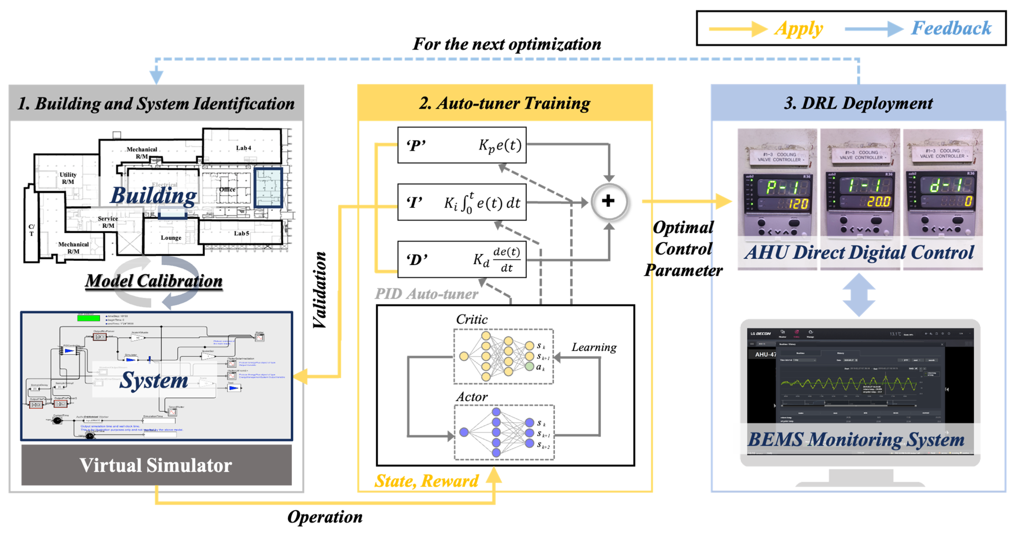
2. Methodology

The proposed process determines the offline tuning PID parameters for an HVAC system control with a deep learning algorithm; this method can be implemented in conventional PID controllers of control systems of existing commercial buildings without major costs. Figure 1 illustrates the overall framework of the research process. The left part shows the building and system identification model to make a reliable simulator by using calibration. The operation data from the model are fed into the PID auto-tuner in the middle part of the figure. In the tuner, a deep reinforcement learning (DRL) model learns the system operation and generates potential control parameters for PID, $K_p$, $K_i$, and $K_d$. DRL evaluates the system performance on energy consumption and indoor air temperature in the simulator model with the generated control parameters. By iterating the process to find the lowest reward of the DRL, the new control parameters are invoked in the direct digital controller of the AHU, and the building energy management system monitors the actual system operations.

2.1. Description of Building and HVAC System

The target building is located in the southwest of central Seoul, Republic of Korea, as shown in Figure 2. The three stories of the commercial building, which was built in the 1980s with a total area of approximately 32,278 m², must be air-conditioned. As a typical multi-functional building, it contains several types of spaces, such as offices, research facilities, a data center, and meeting rooms. The building has 82 air handling unit (AHU) systems with different HVAC types (i.e., constant air volume (CAV) and variable air volume systems) and different installation dates. The target zone is approximately 594 m², and the target AHU is one of the oldest ones in the building as described

Table 1. Specifications of target building.

Element		Parameters
Location		Seoul (Republic of Korea)
Latitude/Longitude		37.46991061154597/127.02686081776729
Building type		Office building
Building scale		B1F/3F
Operation schedule		5:30~19:00
Area	Total (conditioned)	32,278 m2 (22,594 m2)
	Occupancy density	0.11 person/m2
	Target section	594 m2
Composition of envelope (nominal U-value, SHGC)	Wall	Brick [100 mm] + Concrete [200 mm] + Insulation [50 mm] (0.341 W/m2·K)
	Floor	Concrete [200 mm] + Insulation [50 mm] (0.384 W/m2·K)
	Roof	Concrete [100 mm] (0.855 W/m2·K)
	Window	Clear [3 mm] + Air [13 mm] + Clear [3 mm] (2.720 W/m2·K, 0.764) Wall-Window-Ratio = 30% (Strip window)

and

Table 2. Specifications of the HVAC system.

Element	Parameters
Capacity	489.02 kW
Air delivery	CAV (Constant Air Volume)
Air flow rate	2.5 kg/s
Fan pressure	112 mmAQ
Coil type	Cooling and heating water coil
Set-point temperature	Heating: 20 °C, Cooling: 23.5 °C
Plant	Heating: Hot boiler, Cooling: Centrifugal compressor chiller

. Although the control parameters of the heat exchanger valve of the PID controller were adjusted in 2017, the occupants experienced frequent thermal discomfort, in particular during the cooling season.

A building energy management system (BEMS) monitored the energy consumption of the building and the operating status of the primary and secondary systems as shown in Figure 3. Also, the cooling coil valve is controlled by the PID controller with P, I, and D values, respectively, as shown in right side of Figure 3. However, data generated by the BEMS are stored on the database system only for a day, owing to the initial cost limit, which is typical for existing buildings. Due to insufficient operational data for the HVAC system, it is necessary to optimize the system control using short-term datasets.

2.2. Existing HVAC Control System

The target AHU system with CAV has the conventional PID control based on the return air temperature from the conditioned space. The PID controller is a control system that uses proportional, integral, and derivative actions to regulate a process. The controller is commonly used due to its high level of comprehensibility and effectiveness. An advantage of the PID controller is that engineers can easily build the control system, even without an extensive knowledge of control theory, because they have a conceptual understanding of differentiation and integration [25]. Moreover, despite its simplicity, the compensator is remarkably smart since it effectively records the past performance of the system (by integration) and predicts the future dynamics of the system.

In considering the following unity-feedback system in Figure 4, the output of the controller, which can be a input of the AHU system, is able to be calculated in a time domain, as follows:

$$u=K_p\times e+K_j{\int }_0^{t}e dt+K_d\times d\frac{d}{dt}·e$$

(1)

The variable ($e$) denotes the tracking error, which is the discrepancy between the desired ($r$) and the actual output ($y$). The error signal ($e$) is given to the PID controller, and the controller computes both the derivative and the integral of this error signal with each time step. The control signal ($u$) applied to the plant is determined by the sum of three terms: the proportional gain ($K_p$) multiplied by the magnitude of the error, the integral gain ($K_i$) multiplied by the integral of the error, and the derivative gain ($K_d$) multiplied by the derivative of the error.

The control signal ($u$) is applied to the cooling coil valve position, resulting in the acquisition of a new output ($y$). The newly generated output ($y$) is subsequently looped back and compared with the reference value in order to determine the updated error signal ($e$). The controller receives the newly generated error signal and calculates an adjustment to the control input. This procedure persists while the controller is in operation [22] with time step ($s$). The transfer function of a PID controller is obtained by applying the Laplace transform equation [45], as follows:

$$K_p+\frac{K_i}{s}+K_{d}s=\frac{K_d{s}^2+K_{d}s+K_i}{s}$$

(2)

2.3. Virtual Simulator

A model-based optimization process usually requires numerous iterations to determine suitable outputs that are in an acceptable range; a reliable simulation platform is required that imitates the actual operation of the HVAC system and provides comprehensive insights into the thermal interaction between the HVAC system and the air-conditioned space. White and black-box models are the most widely used for the estimation of thermal or energy dynamics in buildings [46].

Although black-box models, which use massive datasets to train models, are very tractable for generating an unknown relationship between inputs (i.e., parameters of the indoor and outdoor conditions of buildings) and outputs (i.e., the consumed energy or indoor temperature), these models are unsuitable for the studied building owing to the lack of historical operation data for the HVAC system. Moreover, domain experts of actual systems sometimes find the models difficult to interpret [47]. Regarding the field operation conditions (i.e., the building is fully occupied), the AHU should not be subjected to downtime during the installation of additional data acquisition equipment or the testing period with different control parameters (P, PI, and PID). Thus, additional training datasets can be generated in operating conditions of the HVAC system with different control parameters. The lack of historical operation data for the single control parameters narrows down the field of investigation and parameter range, which degrades the model performance.

By contrast, white-box models are considered easy to understand (i.e., the engineer can easily understand how each input variable affects the output) and have an adequate explainability–accuracy trade-off [48]. Although the modeling process is complicated owing to the required complete thermo-physical relationships between the space components (i.e., the wall, window, ceiling, and floor) and system operation conditions (e.g., the supply air temperature, valve position, and damper position), it is very practical for determining the effects on the system energy consumption and indoor thermal environment when the control parameters of the HVAC system are changed. In this study, white-box model is more suitable to use as a virtual simulator because it overcomes limitations regarding the data quantity, amount of system operation data, and data quality by operating only with single PID constants.

As shown in Figure 4, the building and system simulator is generated with EnergyPlus (ver. 9.4). Then, the control values of the HVAC system are optimized with an optimization algorithm based on a BCVTB environment. The EnergyPlus is the most widely used whole-building energy simulation program for determining the energy performance characteristics of buildings and system designs, detecting system faults, and managing buildings [49]. The modular architecture of EnergyPlus enables the co-simulation of building energy performance and system operation with other software. When compared to other building energy simulation programs, this program offers a flexible time step control of less than one hour. This is crucial for accurately simulating the HVAC system control in a building [50]. All known building input variables (e.g., the geometry and thermal properties of the building envelope, occupancy density and schedule, lighting and plug load of the as-built and as-used states) were determined with on-site investigations. Other HVAC system information, such as the fan size and type, coil specifications, and air terminals of the operating state, are the input parameters for the simulator.

Two important problems need to be solved; (1) variables that could not be determined in the field investigations, such as infiltration, indoor furniture thermal capacity, degradation of the thermal properties of the building envelope,, should be evaluated to ensure consistency between the simulations and actual operation conditions; (2) EnergyPlus calculates the heating and cooling-energy consumption of the HVAC system to meet the heating and cooling demand of the space in each time step. An additional application process is required to simulate the system response when each PID constant is changed.

A virtual simulator has been calibrated to determine unknown building properties and actual system operation data with the Hooke–Jeeves (HJ) algorithm [51]. The HJ algorithm explores optimal solution with exploratory moves and pattern search given a search space [52]. The exploratory searches and pattern moves continued until there is no improvement in the objective function. The HJ algorithm searches for the best point in a short time (with fewer iterations) compared to other optimization algorithms such as nonlinear programming, quadratic programming, dynamic programming, multi-objective programming, or genetic algorithms [53]. In this research, a small number of unknown parameters that have a significant impact on building energy consumption, a combination of exploratory moves, and a heuristic pattern search-based HJ algorithm might enable the efficient identification of the optimal point within a short time.

The building simulator with HJ algorithm constructed four models with different unknown parameter characteristics in a representative five days within the cooling period as shown in Figure 5; four major factors affecting building energy consumption such as insulation thickness, solar heat gain coefficient (SHGC) from window, infiltration and thermal mass are used for calibration with the HJ algorithm. The calibrated model has a coefficient of variance of the root mean square error (CV(RMSE)) and mean bias error (MBE) with 1-h intervals as suggested in ASHRAE guideline 14, FEMP criteria, and IPMVP [54,55,56]. Among the calibration criteria, calibrated models were evaluated based on the hourly criteria (CV(RMSE) within 30%, MBE within 10%) within ASHRAE guideline 14. Considering the representative period of this study, it was evaluated with CV(RMSE) and MBE indicators in hourly criteria, as follows:

$$CV(RMSE)=\frac{\sqrt{{\frac{1}{n}{\sum }_{t=1}^n{(A}_t-P_t)}^2}}{\overline{A_t}}$$

(3)

$$MBE=\frac{1}{n}\sum _{t=1}^n\left(A_i-P_i\right)$$

(4)

2.4. Deep Deterministic Policy Gradient (DDPG) Algorithm

Reinforcement learning involves experiencing different scenarios within a certain period, assessing the results of the scenarios, taking actions to improve the results, and solving sequential decision-making problems to meet the goal through repeated trials. The agent determines the agent’s action (at) depending on the given state (st); the action causes a change in the next state (st + 1) of the environment, which is communicated back to the agent. In this case, the information about the reward (rt + 1) and state information is transmitted to the agent; reinforcement learning is a continuous decision-making process conducted by the agent, who selects actions that can maximize the reward.

The discrete-time information, t, and likelihoods for the agent to select possible actions for given states in the individual time steps can be expressed as probabilities, which are referred to as “the policy” in reinforcement learning. The policy at time t is expressed as π (st, at); it maximizes the reward of the action decided at time t and all other rewards obtained during the interactions between the environment and actions.

The mathematical expression of this flow is the Markov decision process (MDP); its efficiency is excellent because the decision-making process is based on all historical information [57]. In the MDP, the relationships between individual elements such as the state, action, and reward are expressed probabilistically. The expected value of the value function can be updated by repeating the interaction between the agent and the environment. Regarding reinforcement learning, the method “Q-learning” effectively updates the expected value of the value function. Q-learning is the heart of value-based approaches selected to estimate the Q-value, which is the cumulative discounted reward from the action and state. For the action space and discrete state, the Q-values can be calculated via iterative updates. In addition, the policy gradient method parameterizes the policy function and estimates the value with the gradient of the objective function [58]. In the RL context, this objective is achieved with policy-based or value-based methods.

In practice, the Q-value is usually estimated with a function approximating entity such as a neural network that uses a DQN. Regarding policy-based methods, the policy gradient (PG) algorithm is an important algorithm that improves end-to-end policy by calculating noisy estimations of the expected reward’s gradient and by updating the policy according to the gradient direction. Whenever continuous variables represent the status or action space, a naive alteration of the PG algorithm or DQN through state discretization or the action space usually results in difficulties or sluggish learning convergence and divergence.

The used DDPG algorithm basically combines the value function and policy gradient methods. Parameterizing a policy function and estimating it with the gradient of the objective function is called “the policy gradient method” [59]. The policy has the form of an artificial neural network, and its parameters (i.e., the weight and bias) are updated. During learning, the optimal policy is determined while changing the parameters of the policy neural network. To determine the maximum of $J\left(\theta \right)$, which is the objective function of the policy gradient, $J\left(\theta \right)$ is differentiated by $\theta$, which corresponds to the gradient expression of the objective function. In addition, $\gamma$ is the discount rate, which is used to determine the weight of the present rewards by comparing the future reward, as follows:

$$J\left(\theta \right)=E_{\tau -p_{\theta }\left(\tau \right)}\left[\sum _{k=0}^T{\gamma }^k\gamma \left(s_k,a_k\right)\right]={\int }_{\tau }^T{p}_{\theta }\left(\tau \right)(\sum _{t=0}^T{\gamma }^t\gamma \left(s_k,a_k\right))d\tau$$

(5)

The term (${\sum }_{k=0}^{T }{\gamma }^k\gamma \left(s_k,a_k\right)$) relates to the return in the gradient expression is for all time points; only the return at the current time point t should be considered. Samples can be obtained by generating a trajectory with a policy; this so-called “reinforcement learning” method was developed in Sutton et al. [59]. Updates are impossible as long as the episode has not ended, and the variance of returns is large; nevertheless, the algorithm has become the basis for other policy gradient algorithms. The DDPG algorithm represents the parameterization of actor and critic neural networks into deep neural networks. To obtain the gradient of the objective function of the DDPG algorithm, the action value should be known. That is, the action value function of the Q-value at t policy that $Q^{\pi }(s_t,a_t)$ is estimated with the critical neural network $Q_{\mathrm{\varnothing }}(s_t,a_t)$ with $\mathrm{\varnothing }$ as a parameter. The critic neural network can calculate its time difference target, as follows:

$$Q^{\pi }\left(s_t,a_t\right)=r\left(s_t,a_t\right)+E_{s_{t+1}~p\left(s_{t+1}\right|s_t,a_t)}[E_{a_{t+1}~\pi \left(a_{t+1}|s_{t+1}\right)} \left[\gamma Q^{\pi }\left(s_{t+1},a_{t+1}\right)\right]]$$

(6)

$$y_t=r\left(s_t,a_t\right)+\gamma Q_{\mathrm{\varnothing }}(s_{t+1},{\pi }_{\theta }\left(s_{t+1}\right))$$

(7)

The learning goal is to estimate accurately the action value in Equation (7); the smaller the difference between $y_t$ and $Q_{\mathrm{\varnothing }}(s_t,a_t)$ is, the better the performance of the critic neural network is. In addition, a replay buffer must be used for the DDPG algorithm. The trajectory data $(s_t,a_t,r_t,s_{t+1})$ generated according to the policy are correlated with time. In the DDPG algorithm, the generated data are first stored in the replay buffer; after sufficient data have been collected, the data are sampled and used as learning data. When an agent is trained, it should be able to search the environment effectively. That is, the learning data should be the result of searching the environment by selecting different actions. Since the deterministic policy neural network has no randomness unlike the probability distribution function, the initial action variable is continuously selected. The DDPG algorithm solves this problem by adding noise to the action, which is the result of the actor neural network. As random noise is added, one can break away from the initial value and search the environment while performing different actions [60].

In this study, a specific indoor zone of a commercial building is studied. The indoor temperature in the target zone can be controlled by adjusting its set-point temperature. The CAV system’s AHU system works in the cooling or heating mode according to the indoor temperature and assigned set-point; more specifically, the opening degree of the cooling and heating valve is controlled. The changes in the indoor temperature due to the commercial HVAC control system can be expressed in the form of an MDP.

(1)

State space: the state encompasses relevant information for the decision of control actions, including the setting of the room temperature Tz (t) of the particular zone z and the bound user indoor set-point temperature Tset-point (t). The state parameters include the indoor set-point temperature, which is the control baseline for the valve. The temperature is controlled by opening/closing the valve based on the PID control’s t + 1 time steps that calculate the difference between the indoor and set-point temperatures.

(2)

Action space: the HVAC control method allows the tuning of different parameters, such as the adjustment of the cold-water temperature according to the valve controlling the indoor temperature set point. The valve is controlled via PID control by tuning the Kp, Ki, and Kd parameters. Therefore, the action spaces of this research study are Kp, Ki, and Kd.

(3)

State transition: the state transition probability is not incorporated in the presented MDP because the HVAC system’s thermal dynamic process is influenced by numerous ambiguous factors such as the supply airflow rate, which depends on the mass flow rate of cold water passing through the valve.

(4)

Reward function: the objective of reinforcement learning is maximizing or minimizing the reward cost function. In this study, the reward function is minimized as shown below. The control objectives can be achieved by predetermining the reward of every pair of state and action, such as the optimal temperature control and energy savings, which are the valve opening positions. The probabilities of $\mathsf{\alpha }$ are weighted coefficient values, which are determined during the training of the algorithm, as follows:

$$f(x)={\int }_0^t\left[\left|temperature\left(t\right)-setpoint\right|\right]dt+\alpha \times {\int }_0^{t}valve\left(t\right)dt.$$

(8)

(5)

Building control plan: an optimal HVAC regulator maximizes rewards during the operation of a building. It can also be expressed as a (stochastic) policy that provides a probability distribution over activities while considering the current building status.

The reward function can be modified by the HVAC system type and control schema. The indoor air temperature setting condition, denoted $setpoint$ in Equation (8), can be adjusted by outdoor temperature reset control, which can change the indoor set-point temperature by the outdoor air condition. For the energy consumption term, the cooling or heating coil valve position, denoted $valve\left(t\right)$ in Equation (8), would be replaced the air mass flow or damper position in variable air volume terminals of VAV system.

In this part, the DDPG agent is trained to control the valve opening/closing systems by allowing it to interrelate with the training background that has been fashioned in the earlier temperature step. We designed the simulator and PID controller agent as one framework. The agent chooses the action from the DDPG algorithm; subsequently, the simulator changes the PID constant based on the corresponding action. The DDPG agent’s effectiveness will be determined by the reward it obtains by minimizing the temperature difference with set values and valve opening rates. Also, the thermal comfort level and energy cost are considered with DDPG algorithms.

3. Results

3.1. System Identification by Building Simulator

In order to study the actual operation of a target section of an office building through a simulator and to improve the operating conditions, first, the environment and energy consumption characteristics are investigated for the actual target area. After that, the high level of accuracy of the building simulator is attained by evaluating the estimation of building parameters and calibration performance using the building simulator with the HJ algorithm in the same period.

Figure 5 shows the hourly cooling energy consumption based on representative five days operation data from 1–5 August 2021 during a cooling period compared with the outdoor air temperatures, solar radiation, and cooling energy consumption provided by the initial model with the construction and operation information. During the experimental periods, the average daily temperature and solar radiation were 23.66 °C and 0.66 MJ/m², respectively, and the daily average cooling energy consumption was 119 kWh. Notably, the change in cooling energy consumption does not correlate with the outdoor air temperature and solar radiation under specific criteria during air-conditioned schedules because of the absence of windows and the influence of the room temperature of the adjacent room. The cooling energy consumption has a significant impact on maintaining the set temperature (23.5 °C ± 0.5 °C) in all periods. After that, system identification and calibration of the building simulator in hourly intervals is performed for the representative five weekdays.

The model calibration of the building simulator is a crucial phase for verifying performance of the developed model application of an HVAC system. In this research, four major factors that influence building energy consumption, namely insulation thickness, solar heat gain coefficient (SHGC) from windows, infiltration, and thermal mass, are used for calibration parameters with the HJ algorithm. The calibration performance of hourly cooling energy consumption is measured with different conditions of estimated building parameters during the representative five days, illustrated in Figure 5.

Figure 6 shows the results of correction with the actual cooling energy consumption for each iteration of the virtual simulator (the conditions of estimated parameters presented in

Table 3. Calibration performance of virtual simulator with estimated value of building parameters using HJ algorithm.

		Model 1 (Initial)	Model 2 (Iter.-32)	Model 3 (Iter.-165)	Model 4 (Iter.-540)
Building parameter	Insulation thickness (mm)	90	43	50	62
	SHGC (-)	0.70	0.32	0.65	0.54
	Infiltration (ACH)	1.50	5.70	3.00	3.50
	Thermal Mass (J/kg·m)	5	35	15	10
Calibration performance	CV(RMSE)	0.569	0.422	0.393	0.231
	MBE	−0.905	+0.901	+0.244	+0.087

). Models 1 and 2 differ greatly from the actual values for building energy consumption by more than 50% on average, with respective values of 0.569, −0.905 and 0.422, +0.901 for CV(RMSE) and MBE, respectively, as described in Table 3. The performance degradation of Models 1 and 2 appears to be due to exploring the search space in the initial learning process. However, the calibration performance dramatically improved from +0.901, 0.422 (Model 2) to +0.244, 0.393 (Model 3) for CV(RMSE) and MBE, respectively. This enhancement can be attributed to lower thermal efficiency (i.e., reduced infiltration and thermal mass) and increased SHGC of the window compared to Model 2. Notably, Model 4 outperformed other models with CV(RMSE) of 0.231 and MBE of 0.087, both of which satisfy the hourly acceptance criteria of ASHRAE Guideline 14 (i.e., within 30% for CV(RMSE) and 10% for NMBE). Model 4 demonstrated energy performance similar to real buildings by applying optimal envelope parameters, including reduction in insulation thickness and high infiltration compared to initial condition.

3.2. Validation of Low-Level Control Condition

After correcting the overall energy performance of the virtual simulator, additional verification is necessary to evaluate the operating characteristics of the actual air conditioner with AHU. EnergyPlus can be employed to construct a model of the energy supply level of a building; however, since simulating the actual valve movements is difficult to design, the control performance of coil valve is determined with a co-simulator that can run different simulations, as presented in Section 2.

Figure 7 shows the system operation characteristics according to changes in the individual indicators of the PID controller used for the normalized valve opening rate ($x_{t,norm}$) with scaled features (actual valve opening rate (%), simulator-mass flow rate (kg/s)) through normalization method of raw data ($x_t$), as follows:

$$x_{t,norm}=\frac{x_t-x_{t,min}}{x_{t,max}-x_{t,min}}$$

(9)

During regular daily operations, the cooling coil valve often transitions between a closed state (0) and a completely open state (1) based on the indoor air temperature. During days of high demand, the valve remained fully open to accommodate increased cooling demands. When the control variables ($k_p$, $k_i$, and $k_d$) of actual conditions are used as inputs of a simulator, the room temperature and valve position of the virtual simulator are similar to real conditions for a representative two days (i.e., typical day, peak day) within 0.043 and 0.053, respectively, of CV (RMSE). The simulator shows reliable performance even with irregular valve positions on the peak day. This means that simulator characteristics of the building envelope and HVAC system effectively reflected the actual conditions.

3.3. Convergence of DDPG Algorithm with Control Parameter Estimation

Based on the developed virtual simulator, the valve opening control variables for the cooling coil of the air conditioner can be extracted with the DDPG algorithm, as outlined in Section 2. The configuration of the DDPG algorithm is shown in

Table 4. Configuration of hyperparameter of DDPG algorithm.

Hyperparameter	DDPG
Observation range	(−100, 100)
Action range	(−1, 1)
Optimizer	Adam
Actor learning rate	0.0004
Critic learning rate	0.003
Batch size	128

. In addition, the search range of the target variables ($k_p$, $k_i$ and $k_d$), which are the valve opening control variables, is set from 0 to 10,000 with steps of 0.1 to ensure an adequate range of search steps.

Figure 8 shows the changes in Q-value in the reward function according to the simulation epoch. As the Q-value in the initial state is zero, the Q-value increases when another epoch is added; it converges to 7955 after the epoch reaches 15,000. Ten experiments were performed while changing the initial conditions in the same batch state; the results are similar, and the number of epochs at which the reward values converge is constant.

Table 5. The Q-value in DDPG and control value of PID controllers with each iteration.

	Epoch	Kp	Ki	Kd	Q-Value
Actual	-	20.2	120	0	-
Model (DDPG)	0	0	0	0	1
	3000	0	9.9	1.3	3200
	6000	379.7	0.1	1.2	6600
	9000	168.5	8.5	0.8	7800
	12,000	59.4	9.2	0.1	7850
	15,000	18.7	10	0.01	7955

shows the initial values of the variables and Q-values with different major epochs. The convergence time is approximately three hours, making it feasible to achieve convergence during the period from the end of the air conditioner operation (7:00 p.m.) to the system restart (5:30 a.m.).

Figure 9 shows room temperature with the changes in the valve opening positions driven by $k_p$, $k_i$, and $k_d$ of the DDPG algorithm, as listed in Table 5. The DDPG algorithm explores a feasible boundary with high fluctuations in valve positions during the initial learning process (i.e., iteration = 0–9000). The room temperature shows reliable performance within the boundary after 3000 iterations; however, the fluctuation of the valve opening rate decreased as the training progressed. The room temperature and change of the valve opening positions are more stable with high Q-values, after reaching 9000 iterations. Notably, the $k_d$ values change into zero values after many training epochs. This is because the zone is not so small that it can reflect the control signal right away for the system to change its operation. In the convergence point (i.e., $k_p$ = 18.71, $k_i$ = 10, and $k_d$ = 0.01), room temperature successfully retains the set indoor temperature (i.e., 23.5 ± 0.5 °C) with a low range of valve positions at 0–20%.

3.4. Performance Evaluation Based on Actual Implementation

As described in the previous section, optimal values of the PID controller were determined for target building based on a calibrated virtual simulator. Then the PID controller with auto-tuned parameters ($k_p$, $k_i$ and $k_d$) was tested over ten days in terms of room temperature and cooling energy consumption for cooling periods in this section.

Figure 10 shows the experimental results of the existing PID and auto-tuned PID operating conditions of the HVAC system for the representative two days. The outdoor air conditions of selected representative days showed similar patterns; the daily average outdoor air temperature ranged 19.67–29.90 °C and 21.86–29.10 °C under the existing PID conditions and auto-tuned PID conditions, respectively. The valve opening positions on a daily average are similar to maintaining the indoor set temperature (23.5 ± 0.5 °C) during the building operation at 18.15% and 18.82%, respectively. The variation in the cooling valve opening position of the existing control ranged from 0% to 54.5% at the peak cooling demand. However, the valve position of the auto-tuned PID ranged from 15.4% to 38.2% at the peak. The auto-tuned PID can maintain a stable valve position of less than 20% in the daily cooling operation. It illustrates the existing CAV system may be operating under oversized conditions due to changes in internal load conditions (occupancy, lighting, and plug), and specifies the suggested process that can adopt the HVAC system control to actual indoor thermal responses. In addition, it means that the auto-tuned PID control achieved precise control of indoor thermal comfort with minimal valve opening rate. The room temperature was also stable at 23.62 ± 0.3 °C compared to existing PID operating conditions (i.e., between 22.23 and 24.35 °C). In existing PID conditions, there is a high fluctuation of room temperature because of frequent outdoor air intake. Therefore, the auto-tuned PID control would be a more effective strategy for maintaining indoor comfort with stable operation of the HVAC system.

Figure 11 shows the valve opening rate with actual and improved operating conditions over a 20-day period. The cooling coil opening rate reached a maximum point in a trade-off between return air and fresh outdoor air on most days under both conditions. In a long-term test period, the valve opening positions ranged from zero (i.e., fully closed) to 80.42% under the existing PID operating conditions; it averaged a 19.15% opening rate during operational hours ($\sigma$ = 18.94). On the other hand, the valve opening rate under auto-tuned PID conditions ranged from 10.20% to 43.40%, 17.41% on average ($\sigma$ = 12.08). This can be attributed to the fact that the auto-tuned operating conditions can reduce deviations in the valve opening rate, thereby stabilizing the valve positions.

Figure 12 illustrates the energy consumption of the cooling coil and fan at 15-min intervals under existing and auto-tuned PID conditions for 20 days. Under auto-tuned PID conditions, the cooling coil energy consumption (energy saving rate) reduced by 18 kWh (13.71%) over 10 days, while the fan energy consumption increased by 0.02 kWh (1.77%). The cooling coil achieved the highest daily energy saving of 18.59% compared to existing PID conditions on Day 3, with an outdoor air temperature around 27$\mathrm{℃}$. This is attributed to maintaining a consistent valve opening of the cooling coil with the system’s operating time compared to existing PID conditions. The fan energy consumption remained at an identical level with the system’s operating hours because of the CAV system, which ensured there was no variation in fan power.

The optimal HVAC system is essential to maintaining building energy performance as well as improving indoor thermal comfort. Figure 13 compares the cooling energy consumption averaged daily under the existing PID and auto-tuned PID operating conditions during a period of 20 days. In general, the actual energy consumption of the existing control was higher at 131 kWh than the improved conditions (i.e., 113 kWh) averaged daily. The auto-tuned PID controller can achieve energy savings of 13.71% on all days within the outdoor temperature range of 25–31 °C.

Figure 14 illustrates the distribution of daily room temperature during building operating hours for a period of 20 days. In the existing PID operating conditions, room temperature frequently exceeded the cooling set point temperature compared with auto-tuned PID conditions during experimental periods. Application of the existing system had a range of room temperature from 22.30 °C to 24.40 °C (median temperature—23.41 °C) with high deviations in the air-conditioned schedule; however, when using the auto-tuned system, room temperatures ranged from 23.25 to 23.65 °C (median temperature—23.51 °C) with a stable deviation. Thus, the auto-tuned PID control not only maintained the low energy consumption, but also performed a high level of indoor temperature management. The proposed model provided room temperature satisfaction (23.5 ± 0.5 °C) of 97% in 10 days but, room temperature satisfaction was 49% in existing conditions, as described in

Table 6. The overall performance for building simulator for 10 days.

		Existing PID	Auto-Tuned PID
Cooling coil valve position	Min/Max	0%/80.42%	10.20%/43/40%
	Mean (Standard deviation)	19.15% (18.94)	17.41% (12.08)
Daily averaged cooling energy consumption (saving rate)		131 kWh (-)	113 kWh (13.71%)
Daily averaged room temperature (percentage of satisfied room temperature)		23.36 °C (49%)	23.54 °C (97%)

. In addition, 36% of the room temperature has been maintained at under 23.5 °C, causing unnecessary cooling energy consumption.

4. Discussion

Although this study offered a software-based approach based on reinforcement learning that reduces energy consumption and enhances comfort without requiring significant retrofitting of the CAV system in a typical old commercial building under actual operation, further investigation is required to establish the generalizability and efficacy of the findings. First, it is necessary to apply the suggested approach to other HVAC systems, including VAV, radiant heating and cooling, and packaged air conditioners, to assess energy efficiency and comfort levels. This study exclusively employed the DDPG algorithm for training and optimization. Nevertheless, it is crucial to conduct studies comparing and evaluating diverse reinforcement learning strategies to determine an appropriate model. In addition, integrating a hybrid model configuration incorporating various reinforcement models will accelerate the training process and enhance the efficiency of searching for the global optimum.

5. Conclusions

This study proposes a novel optimization strategy of an AHU system using an auto-tuned PID control method based on a virtual building simulator. The proposed methods can achieve both improved indoor thermal comfort and reduced cooling energy consumption with optimal control parameters of the AHU system. The virtual simulator imitates the operating conditions of an existing building by auto-calibrating the key factors of building energy consumption with HJ algorithm. Then, a low-level control simulator is validated to simulate the actual operation of the AHU system. PID control is combined with a DDPG algorithm to search optimal control parameters. Auto-tuned PID control with a DDPG algorithm was tested with a real-time assessment compared to an existing control without replacing a new valve controller or major retrofitting of HVAC system under downtime.

The proposed control method gave 97% satisfaction of the target temperature range with precise set-point control during cooling periods. Simultaneously, the cooling energy consumption could be reduced by 13.71% with a lower rate of valve operation compared to existing PID operation conditions. It can be observed that the auto-tuned PID control can improve the trade-off between indoor thermal comfort and energy efficiency of HVAC system. The auto-tuned PID control is a relatively simple method to improve efficiency of an HVAC system that is applicable regardless of the system condition and complex maintenance [control actions].

The optimal control strategy has two key improvements. It is essential to assess the impact of frequent changes in the valve operation on the durability and reliability of the system. Although this novel process evaluated thermal energy saving and affordable indoor temperature control for the actual CAV system of an old commercial building, it is necessary to investigate the performance of the suggested system for other building types and different HVAC systems such as VAV, radiant heating and cooling, and packaged air conditioner. Further studies are necessary in two specific areas. It is necessary to enhance overall performance by considering the characteristics of air conditioners and various combinations of fans, economizers, and pumps, especially during the heating season, first. To reduce time and effort, it is necessary to obtain a reliable and robust simulator for each building and system that makes the auto-tuned PID more feasible to apply to an existing building system. Finally, it is necessary to assess generalization performance, not only energy consumption, but sustainability and low global warming gas emissions in other building types and climate conditions.

References

- International Energy Agency. 2021 Global Status Report for Buildings and Construction: Towards a Zero-Emissions, Efficient and Resilient Buildings and Construction Sector; International Energy Agency: Paris, France, 2019. [Google Scholar]
- González-Torres, M.; Pérez-Lombard, L.; Coronel, J.F.; Maestre, I.R.; Yan, D. A review on buildings energy information: Trends, end-uses, fuels and drivers. Energy Rep. 2020, 8, 626–637. [Google Scholar] [CrossRef]
- International Renewable Energy Agency. Global Energy Transformation: A Roadmap to 2050; International Renewable Energy Agency: Masdar City, United Arab Emirates, 2019. [Google Scholar]
- Olivier, J.G.; Schure, K.M.; Peters, J.A.H.W. Trends in global CO2 and total greenhouse gas emissions. PBL Neth. Environ. Assess. Agency 2017, 5, 1–11. [Google Scholar]
- Almusaed, A.; Almssad, A.; Homod, R.Z.; Yitmen, I. Environmental profile on building material passports for hot climates. Sustainability 2020, 12, 3720. [Google Scholar] [CrossRef]
- Goldstein, B.; Gounaridis, D.; Newell, J.P. The carbon footprint of household energy use in the United States. Proc. Natl. Acad. Sci. USA 2020, 117, 19122–19130. [Google Scholar] [CrossRef] [PubMed]
- Li, X.; Ren, A.; Li, Q. Exploring patterns of transportation-related CO2 emissions using machine learning methods. Sustainability 2022, 14, 4588. [Google Scholar] [CrossRef]
- Huang, T.Y.; Huang, P.Y.; Tsai, H.Y. Automatic design system of optimal sunlight-guiding micro prism based on genetic algorithm. Dev. Built Environ. 2022, 12, 100105. [Google Scholar] [CrossRef]
- Jia, L.R.; Han, J.; Chen, X.; Li, Q.Y.; Lee, C.C.; Fung, Y.H. Interaction between thermal comfort, indoor air quality and ventilation energy consumption of educational buildings: A comprehensive review. Buildings 2021, 11, 591. [Google Scholar] [CrossRef]
- Oh, S.; Song, S. Detailed analysis of thermal comfort and indoor air quality using real-time multiple environmental monitoring data for a childcare center. Energies 2021, 14, 643. [Google Scholar] [CrossRef]
- Khare, V.R.; Garg, R.; Mathur, J.; Garg, V. Thermal comfort analysis of personalized conditioning system and performance assessment with different radiant cooling systems. Energy Built Environ. 2023, 4, 111–121. [Google Scholar] [CrossRef]
- Kong, M.; Dong, B.; Zhang, R.; O’Neill, Z. HVAC energy savings, thermal comfort and air quality for occupant-centric control through a side-by-side experimental study. Appl. Energy 2022, 306, 117987. [Google Scholar] [CrossRef]
- Yang, L.; Yan, H.; Lam, J.C. Thermal comfort and building energy consumption implications—A review. Appl. Energy 2014, 115, 164–173. [Google Scholar] [CrossRef]
- Hu, M.; Milner, D. Visualizing the research of embodied energy and environmental impact research in the building and construction field: A bibliometric analysis. Dev. Built Environ. 2020, 3, 100010. [Google Scholar] [CrossRef]
- Gao, Y.; Meng, L.; Li, C.; Ge, L.; Meng, X. An experimental study of thermal comfort zone extension in the semi-open spray space. Dev. Built Environ. 2023, 15, 100217. [Google Scholar] [CrossRef]
- Cao, X.; Dai, X.; Liu, J. Building energy-consumption status worldwide and the state-of-the-art technologies for zero-energy buildings during the past decade. Energy Build. 2016, 128, 198–213. [Google Scholar] [CrossRef]
- Lawrence, T.M.; Boudreau, M.C.; Helsen, L.; Henze, G.; Mohammadpour, J.; Noonan, D.; Patteeuw, D.; Pless, S.; Watson, R.T. Ten questions concerning integrating smart buildings into the smart grid. Build. Environ. 2016, 108, 273–283. [Google Scholar] [CrossRef]
- Dakwale, V.A.; Ralegaonkar, R.V.; Mandavgane, S. Improving environmental performance of building through increased energy efficiency: A review. Sustain. Cities Soc. 2011, 1, 211–218. [Google Scholar] [CrossRef]
- Jung, W.; Jazizadeh, F. Energy saving potentials of integrating personal thermal comfort models for control of building systems: Comprehensive quantification through combinatorial consideration of influential parameters. Appl. Energy 2020, 268, 114882. [Google Scholar] [CrossRef]
- Li, W.; Zhang, J.; Zhao, T. Indoor thermal environment optimal control for thermal comfort and energy saving based on online monitoring of thermal sensation. Energy Build. 2019, 197, 57–67. [Google Scholar] [CrossRef]
- Guo, W.; Zhou, M. Technologies toward thermal comfort-based and energy-efficient HVAC systems: A review. In Proceedings of the 2009 IEEE International Conference on Systems, Man and Cybernetics, San Antonio, TX, USA, 11–14 October 2009; pp. 3883–3888. [Google Scholar]
- Benard, C.; Guerrier, B.; Rosset-Louerat, M.M. Optimal building energy management. Part 2; Control. J. Sol. Energy Eng. 1992, 114, 12–22. [Google Scholar]
- Mathews, E.H.; Arndt, D.C.; Piani, C.B.; Van Heerden, E. Developing cost efficient control strategies to ensure optimal energy use and sufficient indoor comfort. Appl. Energy 2000, 66, 135–159. [Google Scholar] [CrossRef]
- Levermore, G.J. Building Energy Management System: Applications to Low-Energy HVAC and Natural Ventilation Control; E & FN Spon: London, UK, 2000. [Google Scholar]
- Knospe, C. PID control. IEEE Control Syst. Mag. 2006, 26, 30–31. [Google Scholar] [CrossRef]
- Ho, W.K.; Gan, O.P.; Tay, E.B.; Ang, E.L. Performance and gain and phase margins of well-known PID tuning formulas. IEEE Trans. Control Syst. Technol. 1996, 4, 473–477. [Google Scholar] [CrossRef]
- Li, Y.; Ang, K.H.; Chong, G.C. PID control system analysis and design. IEEE Control Syst. Mag. 2006, 26, 32–41. [Google Scholar]
- Valério, D.; Da Costa, J.S. Tuning of fractional PID controllers with Ziegler–Nichols-type rules. Signal Process. 2006, 86, 2771–2784. [Google Scholar] [CrossRef]
- Joseph, E.A.; Olaiya, O.O. Cohen-coon PID tuning method; A better option to Ziegler Nichols-PID tuning method. Eng. Res. 2017, 2, 141–145. [Google Scholar]
- Wang, Q.G.; Lee, T.H.; Fung, H.W.; Bi, Q.; Zhang, Y. PID tuning for improved performance. IEEE Trans. Control Syst. Technol. 1999, 7, 457–465. [Google Scholar] [CrossRef]
- Hamamci, S.E. An algorithm for stabilization of fractional-order time delay systems using fractional-order PID controllers. IEEE Trans. Autom. Control 2007, 52, 1964–1969. [Google Scholar] [CrossRef]
- Moradi, M. A genetic-multivariable fractional order PID control to multi-input multi-output processes. J. Process Control 2014, 24, 336–343. [Google Scholar] [CrossRef]
- Lu, L.I.U.; Liang, S.H.A.N.; Yuewei, D.A.I.; Chenglin, L.I.U.; Zhidong, Q.I. Improved quantum bacterial foraging algorithm for tuning parameters of fractional-order PID controller. J. Syst. Eng. Electron. 2018, 29, 166–175. [Google Scholar] [CrossRef]
- Hussain, S.; Gupta, S.; Gupta, R. Internal Model Controller Design for HVAC System. In Proceedings of the 2018 2nd IEEE International Conference on Power Electronics, Intelligent Control and Energy Systems (ICPEICES), Delhi, India, 22–24 October 2018; pp. 471–476. [Google Scholar]
- Zhao, Y.M.; Xie, W.F.; Tu, X.W. Improved parameters tuning method of model-driven PID control systems. In Proceedings of the 2011 6th IEEE Conference on Industrial Electronics and Applications, Beijing, China, 21–23 June 2011; pp. 1513–1518. [Google Scholar]
- Khodadadi, H.; Dehghani, A. Fuzzy logic self-tuning PID controller design based on smith predictor for heating system. In Proceedings of the 2016 16th International Conference on Control, Automation and Systems (ICCAS), Gyeongju, Republic of Korea, 16–19 October 2016; pp. 161–166. [Google Scholar]
- Karyono, K.; Abdullah, B.M.; Cotgrave, A.J.; Bras, A. The adaptive thermal comfort review from the 1920s, the present, and the future. Dev. Built Environ. 2020, 4, 100032. [Google Scholar] [CrossRef]
- Hussain, S.; Gabbar, H.A.; Bondarenko, D.; Musharavati, F.; Pokharel, S. Comfort-based fuzzy control optimization for energy conservation in HVAC systems. Control. Eng. Pract. 2014, 32, 172–182. [Google Scholar] [CrossRef]
- Satrio, P.; Mahlia, T.M.I.; Giannetti, N.; Saito, K. Optimization of HVAC system energy consumption in a building using artificial neural network and multi-objective genetic algorithm. Sustain. Energy Technol. Assess. 2019, 35, 48–57. [Google Scholar]
- Kang, W.H.; Yoon, Y.; Lee, J.H.; Song, K.W.; Chae, Y.T.; Lee, K.H. In-situ application of an ANN algorithm for optimized chilled and condenser water temperatures set-point during cooling operation. Energy Build. 2021, 233, 110666. [Google Scholar] [CrossRef]
- Sangi, R.; Müller, D. A novel hybrid agent-based model predictive control for advanced building energy systems. Energy Convers. Manag. 2018, 178, 415–427. [Google Scholar] [CrossRef]
- West, S.R.; Ward, J.K.; Wall, J. Trial results from a model predictive control and optimisation system for commercial building HVAC. Energy Build. 2014, 72, 271–279. [Google Scholar] [CrossRef]
- Li, W.; Wang, S.; Koo, C. A real-time optimal control strategy for multi-zone VAV air-conditioning systems adopting a multi-agent based distributed optimization method. Appl. Energy 2021, 287, 116605. [Google Scholar] [CrossRef]
- Fang, X.; Gong, G.; Li, G.; Chun, L.; Peng, P.; Li, W.; Shi, X.; Chen, X. Deep reinforcement learning optimal control strategy for temperature setpoint real-time reset in multi-zone building HVAC system. Appl. Therm. Eng. 2022, 212, 118552. [Google Scholar] [CrossRef]
- Barbosa, R.S.; Machado, J.T.; Ferreira, I.M. Tuning of PID controllers based on Bode’s ideal transfer function. Nonlinear Dyn. 2004, 38, 305–321. [Google Scholar] [CrossRef]
- Arendt, K.; Jradi, M.; Shaker, H.R.; Veje, C. Comparative analysis of white-, gray-and black-box models for thermal simulation of indoor environment: Teaching building case study. In Proceedings of the 2018 Building Performance Modeling Conference and SimBuild Co-Organized by ASHRAE and IBPSA-USA, Chicago, IL, USA, 26–28 September 2018. [Google Scholar]
- Rudin, C. Stop explaining black box machine learning models for high stakes decisions and use interpretable models instead. Nat. Mach. Intell. 2019, 1, 206–215. [Google Scholar] [CrossRef]
- Gupta, S.; Bagga, S.; Sharma, D.K. Intelligent Data Analysis: Black Box Versus White Box Modeling. In Intelligent Data Analysis: From Data Gathering to Data Comprehension; Wiley: Hoboken, NJ, USA, 2020; pp. 1–15. [Google Scholar]
- Jradi, M.; Sangogboye, F.C.; Mattera, C.G.; Kjærgaard, M.B.; Veje, C.; Jørgensen, B.N. A world class energy efficient university building by danish 2020 standards. Energy Procedia 2017, 132, 21–26. [Google Scholar] [CrossRef]
- Zhu, D.; Hong, T.; Yan, D.; Wang, C. A detailed loads comparison of three building energy modeling programs: EnergyPlus, DeST and DOE-2.1 E. In Building Simulation; Springer: Berlin/Heidelberg, Germany, 2013; Volume 6, pp. 323–335. [Google Scholar]
- Khadanga, R.K.; Padhy, S.; Panda, S.; Kumar, A. Design and analysis of multi-stage PID controller for frequency control in an islanded micro-grid using a novel hybrid whale optimization-pattern search algorithm. Int. J. Numer. Model. Electron. Netw. Devices Fields 2018, 31, e2349. [Google Scholar] [CrossRef]
- Bagirov, A.M.; Barton, A.F.; Mala-Jetmarova, H.; Al Nuaimat, A.; Ahmed, S.T.; Sultanova, N.; Yearwood, J. An algorithm for minimization of pumping costs in water distribution systems using a novel approach to pump scheduling. Math. Comput. Model. 2013, 57, 873–886. [Google Scholar] [CrossRef]
- KIRGAT, M.G.; Surde, A.N. Review of Hooke and Jeeves Direct Search Solution M Ethod Analysis Applicable to Mechanical Design Engineering. Int. J. Innov. Eng. Res. Technol. 2014, 1, 1–14. [Google Scholar]
- ASHRAE. ASHRAE Guideline 14-2002 for Measurement of Energy and Demand Savings. In American Society of Heating, Refrigeration and Air Conditioning Engineers; ASHRAE: Atlanta, GA, USA, 2002. [Google Scholar]
- FEMP-US Department of Energy Federal Energy Management Program. M & V Guidelines: Measurement and Verification for Performance-Based Contracts Version 4.0; FEMP—Federal Energy Management Program: Washington, DC, USA, 2015. Available online: https://www.energy.gov/eere/femp/downloads/mv-guidelines-measurement-and-verification-performance-based-contracts-version (accessed on 20 May 2023).
- IPMV—International Performance Measurement & Verification Protocol. “Concepts and Options for Determining Energy and Water Savings”. In Handbook of Financing Energy Projects; EVO—Efficiency Valuation Organization: Toronto, ON, Canada, 2012. [Google Scholar]
- Si, B.; Tian, Z.; Chen, W.; Jin, X.; Zhou, X.; Shi, X. Performance assessment of algorithms for building energy optimization problems with different properties. Sustainability 2018, 11, 18. [Google Scholar] [CrossRef]
- Sutton, R.S.; Barto, A.G. Introduction to Reinforcement Learning; MIT Press: Cambridge, MA, USA, 1998; Volume 135, pp. 223–260. [Google Scholar]
- Sutton, R.S.; McAllester, D.; Singh, S.; Mansour, Y. Policy gradient methods for reinforcement learning with function approximation. Adv. Neural Inf. Process. Syst. 1999, 12, 1057–1063. [Google Scholar]
- Lillicrap, T.P.; Hunt, J.J.; Pritzel, A.; Heess, N.; Erez, T.; Tassa, Y.; Silver, D.; Wierstra, D. Continuous control with deep reinforcement learning. arXiv 2015, arXiv:1509.02971. [Google Scholar]