Abstract
In this study, the extent of concrete building distress is used to determine whether a building needs to be demolished and maintained, and the study focuses on accurately identifying target distress in different complex contexts and accurately distinguishing between their categories. To solve the problem of insufficient feature extraction of small targets in bridge disease images under complex backgrounds and noise, we propose the YOLOv8 Dynamic Plus model. First, we enhanced attention on multi-scale disease features by implementing structural reparameterization with parallel small-kernel expansion convolution. Next, we reconstructed the relationship between localization and classification tasks in the detection head and implemented dynamic selection of interactive features using a feature extractor to improve the accuracy of classification and recognition. Finally, to address problems of missed detection, such as inadequate extraction of small targets, we extended the original YOLOv8 architecture by adding a layer in the feature extraction phase dedicated to small-target detection. This modification integrated the neck part more effectively with the shallow features of the original three-layer YOLOv8 feature extraction stage. The improved YOLOv8 Dynamic Plus model demonstrated a 7.4 percentage-point increase in performance compared to the original model, validating the feasibility of our approach and enhancing its capability for building disease detection. In practice, this improvement has led to more accurate maintenance and safety assessments of concrete buildings and earlier detection of potential structural problems, resulting in lower maintenance costs and longer building life. This not only improves the safety of buildings but also brings significant economic benefits and social value to the industries involved.
1. Introduction
Bridge construction is indispensable in today’s social development, but with the passage of time and the impact of natural disasters, most bridges are subject to different degrees of damage [1]. We can detect apparent bridge damage, speculate on the degree of damage, and thus repair the diseased bridge in time to ensure the structural safety of bridge construction [2] and service life. Apparent bridge damage can be divided into five categories: cracks, corrosion, spalling, weathering, and exposed tendons [3]. The traditional bridge disease detection methods mostly use manual detection, and for cracks, exposed tendons of this type of disease can allow better discrimination. However, for corrosion, spalling, and weathering of similar diseases, human judgments are subjective. Due to the large amount of data, manual detection workload, slow detection, and high leakage rate [4], manual detection is no longer used as the mainstream method of apparent bridge disease detection.
With drone equipment used for manual picture data acquisition and detection [5], digital image processing technology has been developed in parallel with the times, and deep learning-based detection in particular has become a research hotspot in the field of detection [6]. For example, Jahanshahi [7] used neural networks to detect cracks and experimentally verified that the accuracy of his scheme was 79.5%, which was higher than the accuracy of 78.3% using support vector machines. However, there was no significant improvement in the detection of types of distress other than cracks. Hoskere et al. [8] introduced a parallel neural network based on semantic segmentation for the classification of distress and achieved automatic detection of six different types of distress: cracks in concrete, spalling, exposed steel reinforcement, corrosion of steel, fractured cracks in steel, and cracks in asphalt. However, there was no clear determination for corrosion or weathering. Song [9] improved the RPN anchor window design and the RPN anchor window screening of Soft-NMS based on Faster-RCNN and realized an improvement of 3.28% in average classification recognition accuracy for four types of concrete construction damages, namely, cellular pockmarking, whitish segregation, cracking, and corrosion. However, that system does not accurately recognize large-area lesions such as spalling, where the foreground and background are difficult to distinguish, thus requiring improvements to the network or feature extraction module. For example, Mu [10] proposed an adaptive layer-attention network based on the YOLOv5 target detection frame to improve the accuracy of detecting surface defects on steel structures [11] in concrete buildings. In this context, the graph convolutional network (GCN) method proposed by Chen [12] provides new ideas for the prediction of networks, which not only help in understanding the effects on concrete structures but may also provide valuable references for the prediction of other types of structural damage.
2. Related Work
The core idea of the YOLO algorithm is to transform the target detection problem into a regression problem [13]. Because the YOLO series involves end-to-end training, is trained directly on the entire network structure, and has global context information, few localization errors, multi-scale features, and strong handling of small targets, the YOLOv8 [14] network was chosen to study bridge diseases. It can effectively improve the detection accuracy and efficiency and provide a new, advanced detection method for the engineering field.
Challenges of the existing methods are given below.
(1) Difficulty in separating foreground and background. Traditional bridge disease detection methods do not perform well in dealing with complex background or foreground overlapping problems. This is because in the case of some diseases (e.g., spalling, weathering, etc.), the color, texture, and other features of the damaged area and the background area are very similar, making it difficult for the model to accurately differentiate them.
(2) Uneven distribution of diseases. Bridge diseases are usually distributed in different ways, and some may be small areas of spot damage while others are large areas of spalling or weathering. This uneven distribution poses a challenge to the model used for detection.
(3) Detection of small targets. Small targets (e.g., fine cracks) in areas of bridge distress are often missed by detection models, especially in conventional models, because of their weak ability to recognize small targets.
Aiming to address the current problems, such as superposition of bridge disease types, difficulty in separating foreground and background, and uneven distribution of diseases, to improve the recognition accuracy of various types of diseases, we propose a new YOLOv8 model, YOLOv8 Dynamic Plus, based on contextual information and features. The main improvements are as follows.
(1) Improved C2f module. Traditional convolution modules may introduce computational bottlenecks when dealing with large-kernel convolution while making it difficult to effectively capture detailed information. The effect of large-kernel convolution is enhanced by introducing parallel dilution convolution and structural reparameterization. This approach helps in better handling the subtle differences between foreground and background and improving the prediction accuracy of the bounding box.
(2) Task-aligned dynamic detection head (TADDH) structure. Classification and localization tasks usually require different features, but traditional models may have conflicting feature selection between the two. The TADDH structure aims to select features dynamically, thus facilitating consistency between classification and localization tasks. This approach helps in ensuring that the model can optimize both classification and localization performance during the detection process.
(3) Addition of small-target detection layer. The detection rate of small targets is insufficient, especially when the target is mixed with the background, and traditional models may struggle to accurately recognize these small targets. The addition of a layer dedicated to small-target detection in the neck of the network helps to improve the detection rate of small targets and addresses the shortcomings of traditional models in small-target recognition.
3. The Algorithms in This Study
3.1. Overall Improvements Based on the YOLOv8 Network
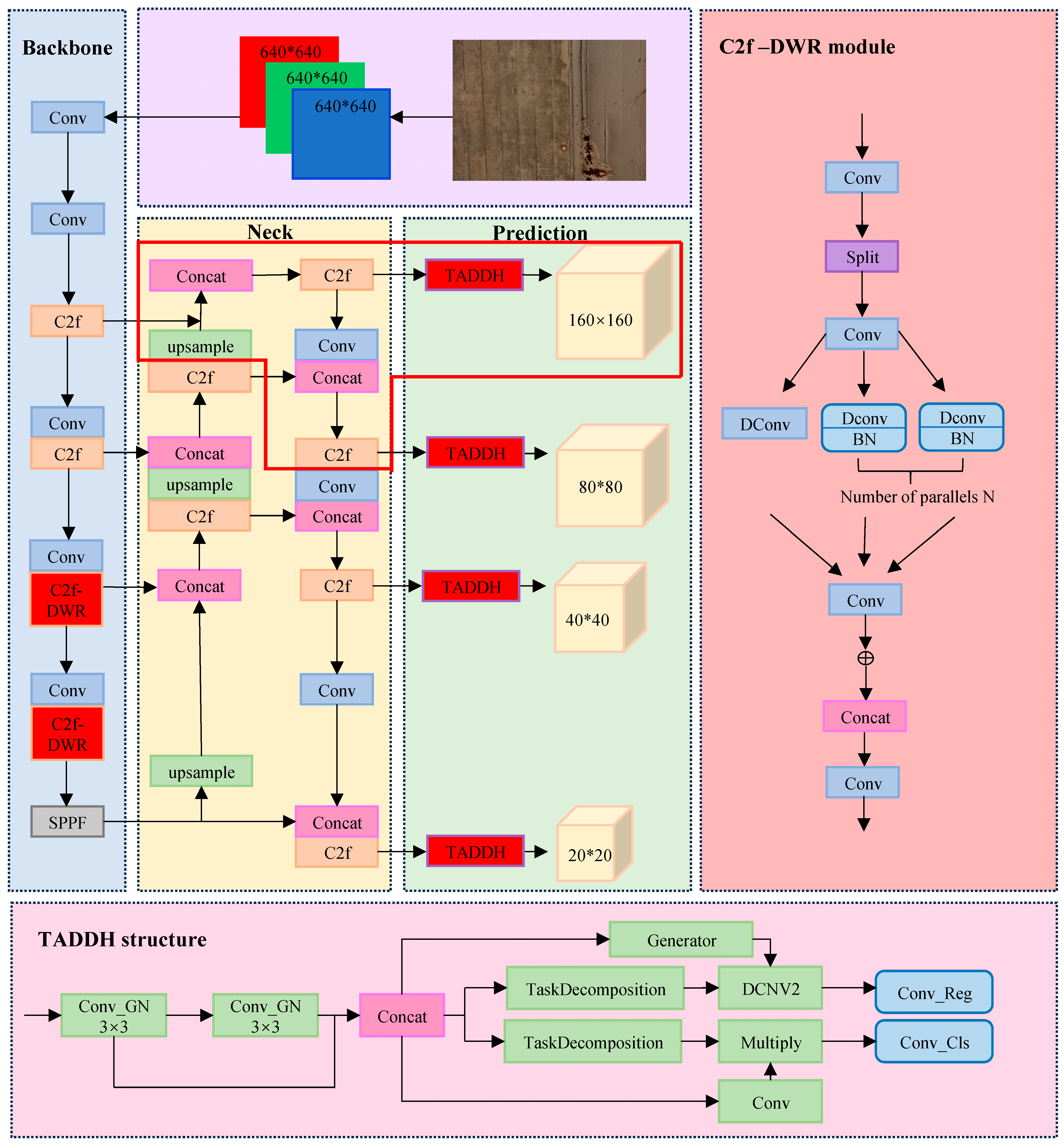
The improvement of the YOLOv8 network is divided into three main parts: backbone, neck, and prediction. Its specific structure is shown in Figure 1.
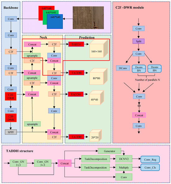
Figure 1.
Structure of the YOLOv8 Dynamic Plus model.
3.2. Backbone Network Improvements
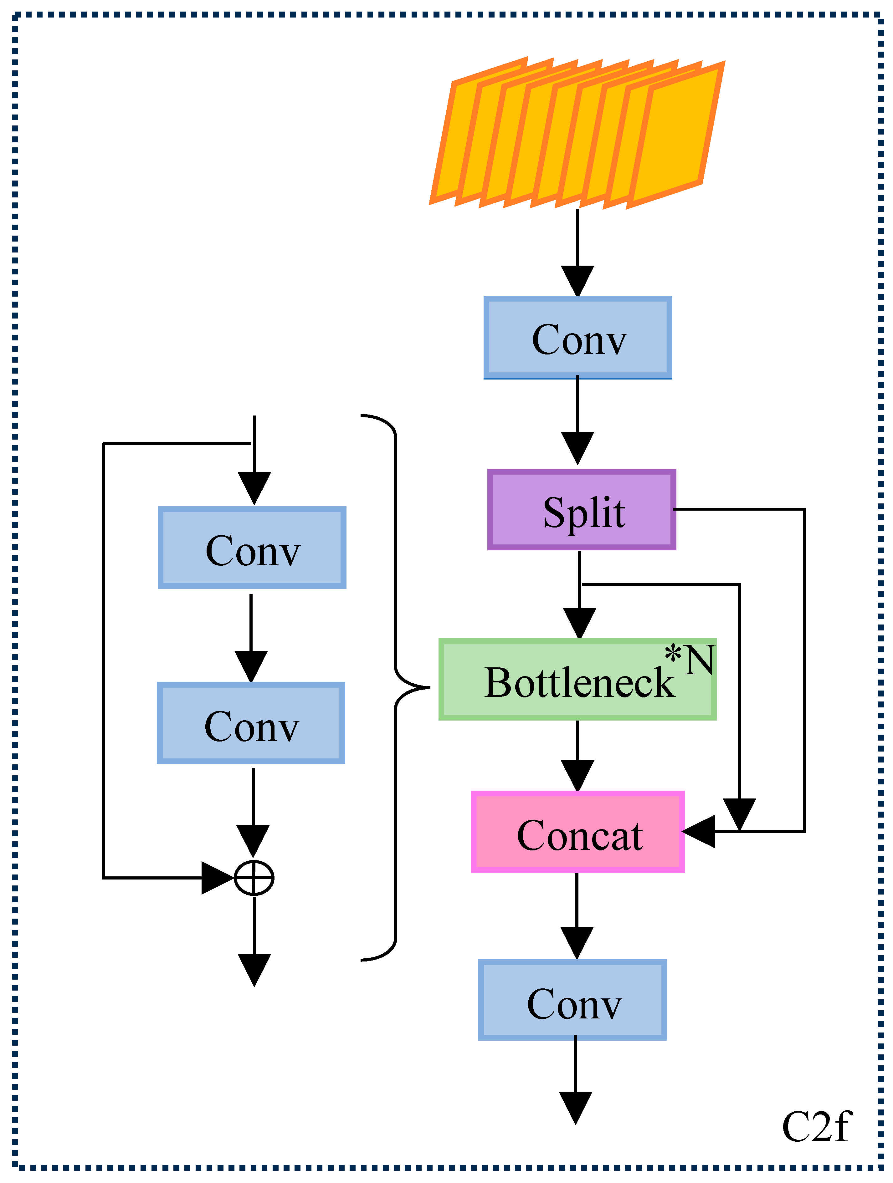
The Backbone part of YOLOv8 uses SPPF and C2f modules. The Channel through the Bottleneck input Tensor is split by 3 × 3 convolution, and the output is reduced to 0.5 times of the previous level, which increases the jump connections and significantly reduces the computational complexity, as well as enhances the sensitivity and accuracy of the details of the bridge disease. This is crucial for processing a large amount of image data and real-time detection. The specific structure is shown in Figure 2.
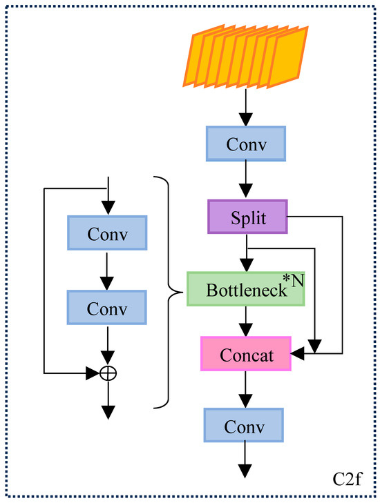
Figure 2.
Structure of the C2f module.
However, this design may weaken the connection between the disease region and the background, while the traditional depth-space dilation convolution can only capture single multi-scale feature information, with limited learning effect of large dilation rate weights, and it is difficult to acquire contextual information.
For this reason, the dilation-wise residual (DWR) structure is introduced into the C2f module. The DWR structure is shown in Figure 3. The core of the DWR structure is to utilize multi-scale extended convolution to capture contextual information at different scales. Different from the traditional extended convolution, DWR improves the accuracy of feature extraction through the ideas of regional residualization and semantic residualization. In this way, DWR can effectively avoid the limitations of traditional depth-space extended convolution when dealing with bridge diseases, especially in capturing multi-scale features.
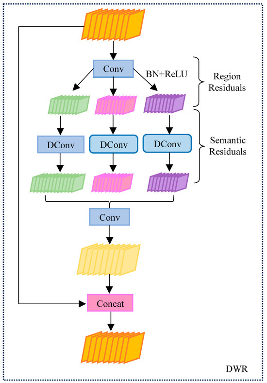
Figure 3.
Schematic diagram of DWR structure.
A single DWR structure is limited by its kernel size and expansion rate, which may not be able to adequately capture small and discrete features or efficiently identify some localized features. To address these limitations, the dilated reparam block (DRB) is used. The improved structure is shown in Figure 4.
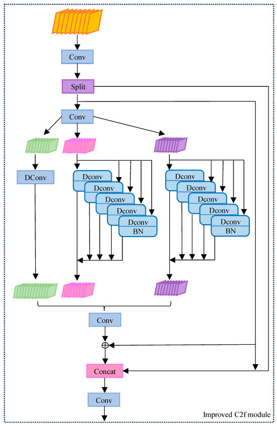
Figure 4.
Improved structure of the C2f module.
DRB combines a non-inflated small kernel and multiple inflated small-kernel layers to augment a non-inflated large-kernel convolutional layer. It can capture more detailed feature information without adding additional computational burden, which significantly improves the detail sensitivity in bridge disease detection. It can be represented as:
where is a convolution operation with expansion rate , ReLU is a modified linear unit, Input is the input of the module, and Output is the output of the module.
Specifically, by using multiple convolutional branches with different expansion rates in parallel and combining a batch normalization (BN) layer [15] into the convolutional layer, the DRB is enabled to efficiently expand the receptive field while retaining sensitivity to details. For different types of lesions or defects, DRB can better handle information of different sizes and complexities through its flexible kernel size and expansion rate settings, further enhancing the performance of the model.
3.3. Improvements to the Header Network
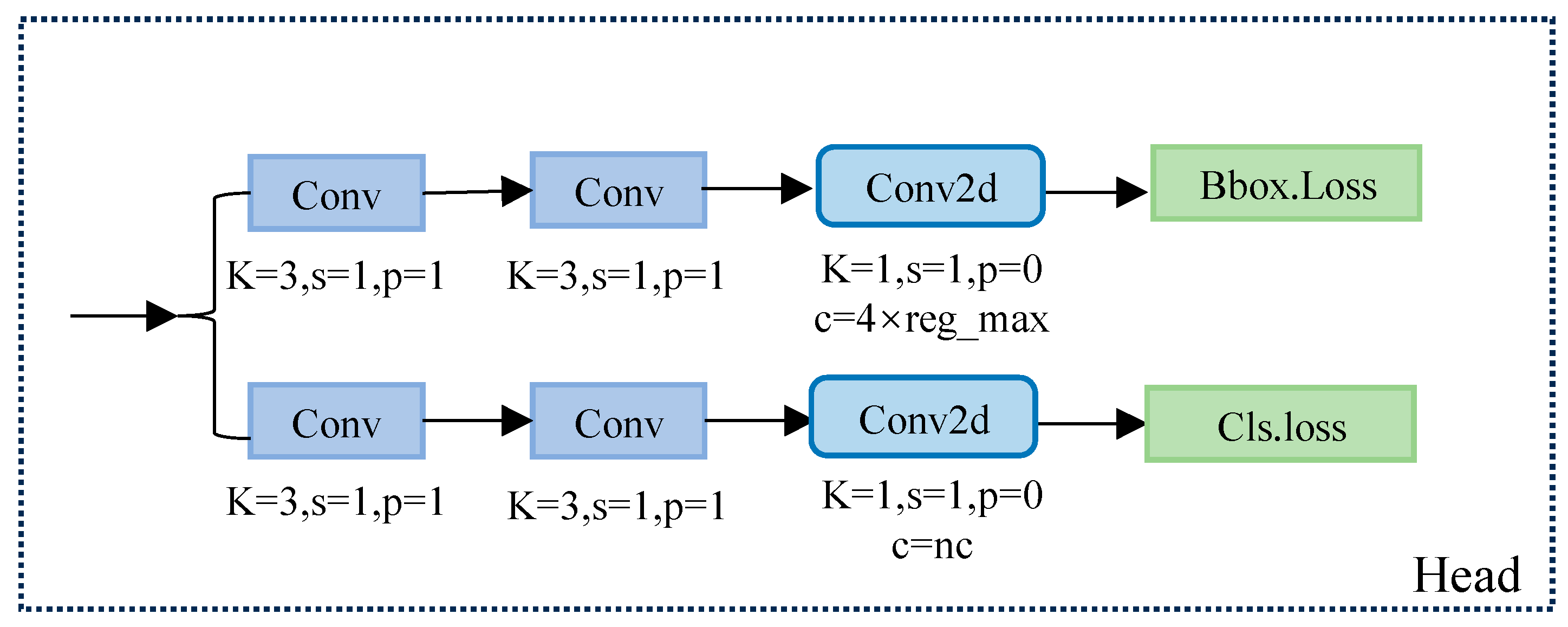
In the YOLOv8 detection head part, the decouple-head structure is used. Decouple head separates the target classification and bounding box regression tasks, with independent modules for each task, as a way to improve the interpretability of the model and optimize the task-specific loss function.
Specifically, it first branches through two CBS convolutional modules, which independently handle the classification and bounding box regression tasks. Next, a Conv2d layer is passed through to integrate the features and finally produce two independent loss values: classification loss and bounding box loss. The classification loss usually uses the binary cross-entropy (BCE) loss function, while the bounding box loss combines improved cross-parity ratio loss (CioU) and distributed focus loss (DFL) to measure the difference between the predicted frame and the true frame. The structure is shown in Figure 5.
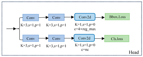
Figure 5.
Schematic diagram of the decouple-head structure.
In the traditional decouple-head design, the target detector uses independent classification and localization branches, which may lead to a lack of effective interaction information between the two tasks, thus affecting the final detection accuracy. To solve the problem of mismatch between classification and localization tasks in traditional single-stage target detection models, the task-align dynamic detection head (TADDH) structure is designed.
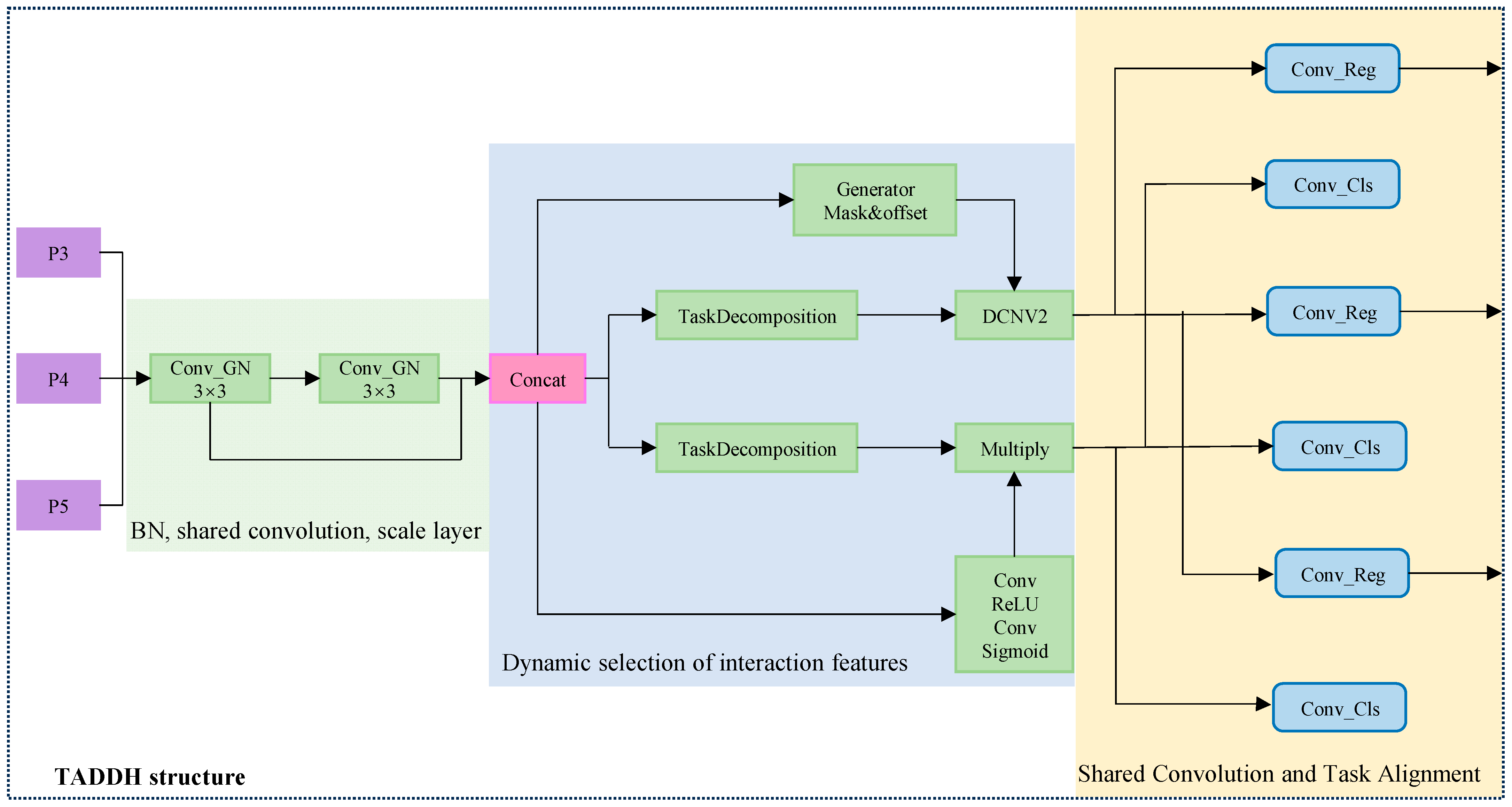
The TADDH combines a hierarchical attention mechanism and a task interaction feature alignment method, which can better adapt to the targets of different sizes and shapes by dynamically adjusting the parameters of the detection head, especially for small targets such as bridge diseases. The accuracy and efficiency of bridge disease detection feature recognition are effectively improved, and false positives and false negatives are reduced. It also further enhances the interaction information between the classification task and the localization task to adapt to the complex background and the diversity of target morphology in specific disease detection scenarios, making the model more practical and accurate in practical applications. Its structure is shown in Figure 6.
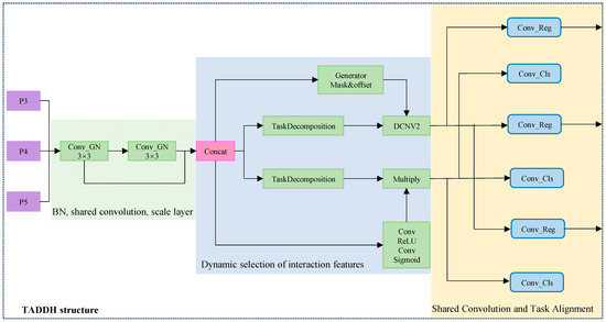
Figure 6.
Schematic diagram of TADDH structure.
3.3.1. Introducing Label Assignment Positioning Alignment Tasks
Bridge disease detection usually involves both classification and localization tasks. Classification and localization tasks are often handled independently, which may lead to poor information flow and affect the synergistic effect between tasks. Due to the conflict of feature selection, it may also lead to a decrease in model performance when optimizing classification and localization at the same time, affecting the overall detection accuracy. The introduction of the label assignment strategy alignment task allows the detector to more accurately identify bridge lesions while also performing the localization task on the detection head. The interaction features are effectively utilized to ensure synergy between the classification and localization branches and to avoid the problem of information isolation caused by traditional independent branches. The hierarchical attention mechanism, formulated as shown below, optimizes the prediction results of both tasks simultaneously, resulting in more consistent and reliable information for classification and localization:
where and are two fully connected layers, is the activation function, and is the cascade feature obtained by average pooling of :
where is a cascade feature of , is a 1 × 1 convolution used for dimensionality reduction, and is a dense classification score transformed with sigmoid or a prediction frame size in the regression task. This results in the alignment of the classification and localization tasks.
3.3.2. Adding Shared Convolution and Scaling Features Using Scale Layer
Bridge diseases manifest in a variety of ways, including defects or damages of different sizes, shapes, and locations. Traditional models may have inconsistencies in feature extraction at different locations, which can easily lead to model overfitting and reduce the generalization ability, and often fail to dynamically adjust the feature response when dealing with defects of different sizes, which may lead to the omission of detecting small targets and misdetection of large targets. The shared convolution layer can effectively extract features from different locations and avoid learning each location individually, thus reducing the risk of overfitting and enhancing the generalization ability of the model. Assuming that the input feature map is , the convolution kernel is , and the output feature map is , then the computation of shared convolution can be expressed as:
where denotes the result of applying the convolution kernel at position (i, j) to the input feature map .
In addition, the scale layer can dynamically adjust the weights and response strengths of the features according to the size and importance of the disease. The specific formula is as follows:
where is the input feature, is the output feature, and and are the parameters of the scale layer, which are used to scale and offset the input features, respectively.
For the bridge disease region to be detected, the scale layer enhances the response of the feature map, which helps the large target features to be detected more accurately. For small or unimportant diseases, the feature response is weakened to reduce the false-detection rate. The combination of shared convolution and scale layer is not only suitable for the complex task of bridge disease detection but also can optimize the model structure and improve the detection accuracy and efficiency.
3.3.3. Replace Batch Normalization (BN) with Group Normalization (GN)
In the bridge disease detection network training, it was found that the performance of BN is highly affected by the batch size, and smaller batches may lead to inaccurate estimation, which requires special treatment to adapt to the single-sample input in the inference stage in practical applications.GN. On the other hand, it is better suited to cope with feature maps of different sizes in its design, and instead of relying on the statistics of the whole batch as BN does, the feature maps are partitioned into multiple groups for normalization, which is particularly important for complex bridge disease detection tasks.
Assume that the input features are , divided into groups, and each group contains feature channels, where is the total number of feature channels. For each group , the mean and variance are calculated:
where and are the height and width of the feature map, respectively, and is a very small constant (preventing division by zero).
The resulting mean and variance are then made normalized for each group :
Finally, apply scaling and displacement for each feature channel yields:
where is the output feature after GN, and and are the learnable parameters.
Replacing BN with GN improves the model’s adaptability to small batches and single samples, enhances the ability to handle different feature map sizes, improves the model’s generalization ability, and enhances the computational efficiency. This makes GN particularly suitable for dealing with the complex task of detecting bridge diseases, and thus the model is more reliable and efficient in practical applications.
3.3.4. Dynamic Selection of Interaction Features
The shape and size of the convolution kernel of the traditional model are fixed and cannot adapt to the complex shape and deformation of the target object, which will limit the ability to detect bridge diseases. Moreover, the traditional model cannot dynamically adjust the feature extraction strategy according to different tasks, so it may not be flexible or precise enough in dealing with features of different bridge diseases. In contrast, deformable convolutional network v2 (DCNV2) adapts the convolutional kernel with learnable offset and shape parameters so that it can adapt to complex target shapes and improve the detection accuracy of bridge lesions.
Using the interaction features obtained from the feature extractor, DCNV2 and the interaction features are used on the localization branch to generate offsets and masks to enable dynamic feature selection for classification and localization tasks.
For the input feature , the output of the deformable convolution can be expressed as:
where is the spatial location in the output feature map , is the offset, and is the learnable convolutional kernel weights.
Instead of extracting directly from the feature map, DCNV2 uses additional convolutional layers to generate , and these offsets are trained to adaptively capture information about non-uniform sampling points of the target object. A learnable shape parameter is introduced to adjust the shape of the convolutional kernel to better fit the feature structure at different locations. Meanwhile, backpropagation is optimized to efficiently learn the offsets and the shape parameters and maintain the stability of the gradient.
The dynamic calculation of different task-specific features through the formula helps in performing task decomposition between different tasks and can adjust the feature extraction process according to the task requirements, which reduces the interference between task features and improves the accuracy and efficiency of the task.
TADDH can align the predicted results of classification and localization through task-interacting features, enhancing the flow of information between the classification and localization branches, and thus improving the overall detection accuracy. Dynamic feature adjustment enables it to adapt to different types of bridge diseases and environmental conditions, allowing the model to cope with a variety of complex scenarios and conditions.
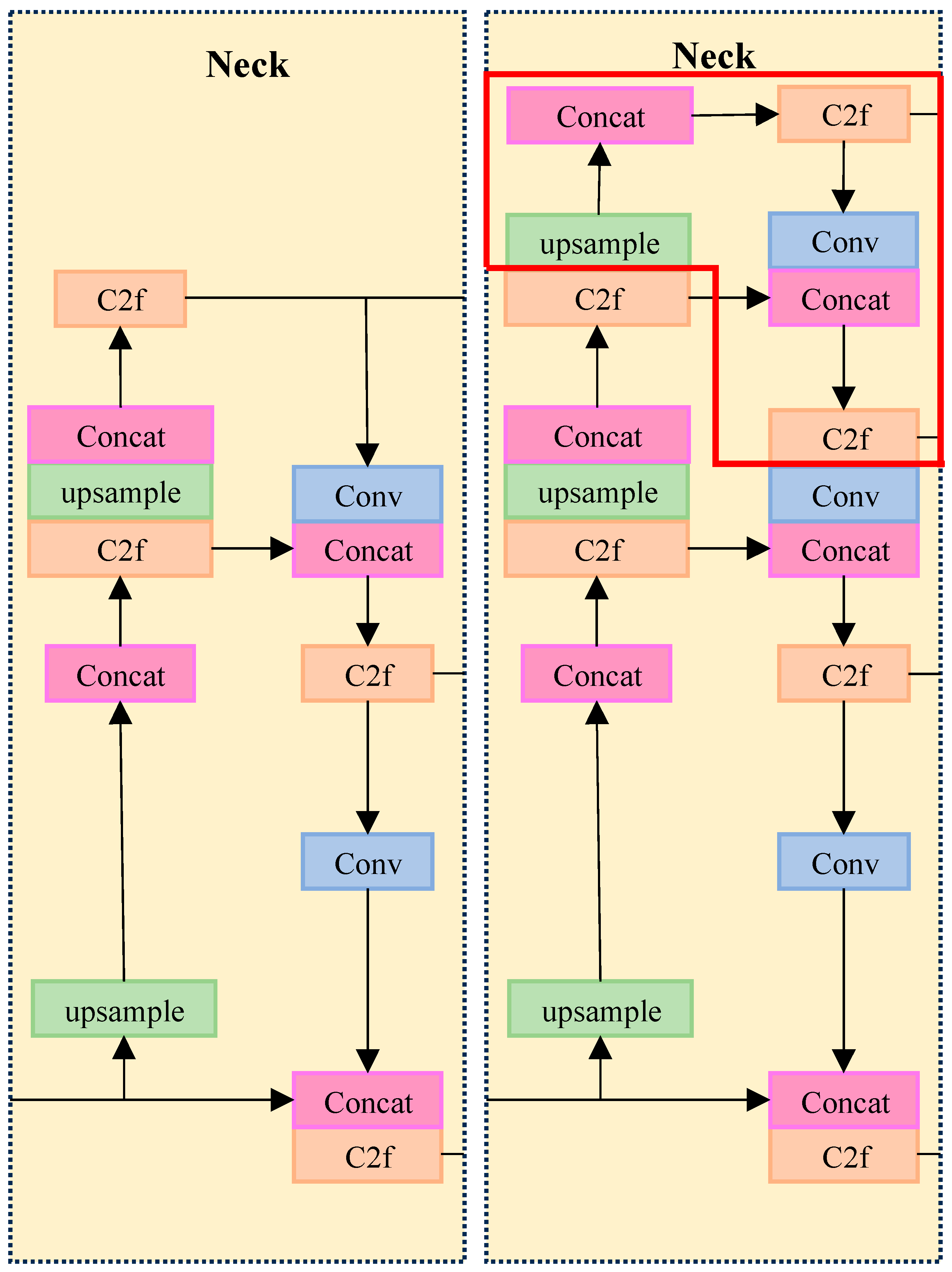
3.4. Improvements to the Neck Network
For the current improvement, after analyzing the network structure, it was found that the FPN and PAN structures of the YOLOv8 network had missing information in most of the vertical connections during feature fusion, as the number of network layers increased and could not fuse the information effectively. This leads to the problem of difficult extraction of small target diseases, low intersection and merger ratio, and poor detection accuracy.
To solve this problem, we propose adding an operational layer for the extraction of smaller targets to the YOLOv8 detection layer of the PANet network for up-sampling. The inputs of the PANet structure are extended with an additional Layer2 layer that is downsampled by a factor of 4 on top of the original Layer9, Layer6 and Layer4 layers. This structure not only incorporates shallower information and improves the accuracy of location information but also enhances the stability of training and the accuracy of the model. The specific improvement scheme is shown in Figure 7.
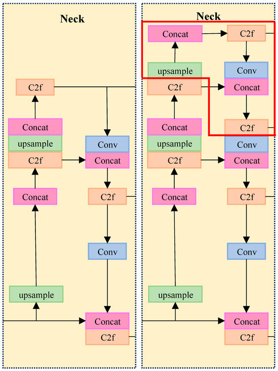
Figure 7.
Comparison of the two structures of the added detection layer and the original YOLOv8 neck.
Traditional models may suffer from training instability during the training process, especially when dealing with complex or fine targets, leading to poor performance of the final model. The advantage of this approach is that adding a specialized extraction layer for small targets not only helps to improve the accuracy of the target frame but also effectively increases the ability to extract the positional information of small targets, thus improving the overall detection accuracy and intersection ratio.
4. Experimentation and Analysis
4.1. Experimental Environment and Dataset
This study is based on deep learning for bridge disease detection, and the model training was tested on a Linux system server. The hardware and software configurations are shown in Table 1.

Table 1.
Hardware and software configurations.
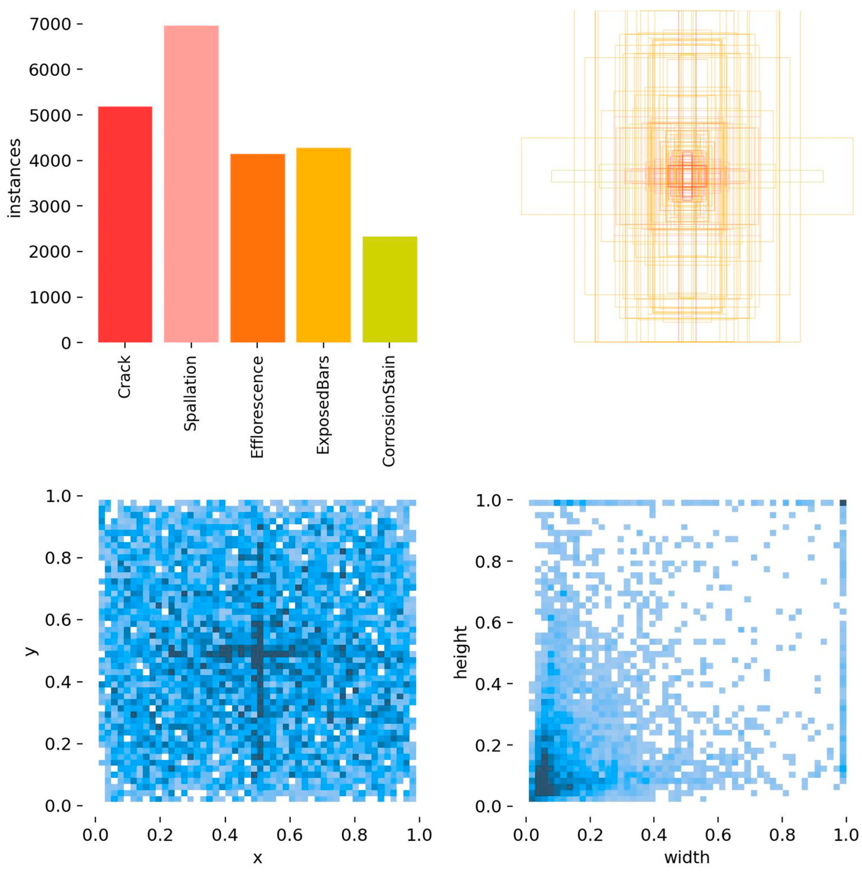
The base dataset in the experiment was the bridge disease public dataset CODEBRIM: Concrete Defect Bridge Image Dataset, published in 2019 for bridge concrete defect detection of multi-targeted diseases in computer vision and machine learning. The dataset contains five bridge defects: cracks, weathering, exposed reinforcement, corrosion, and spalling. A total of 1022 images and 5354 annotated disease bounding boxes are included. Data enhancement was performed on this dataset for sample expansion, and the expanded dataset totaled 4096 images, of which a total of 29,300 real disease boxes were labeled. The labeling types and the number and size of boxes are shown in Figure 8.
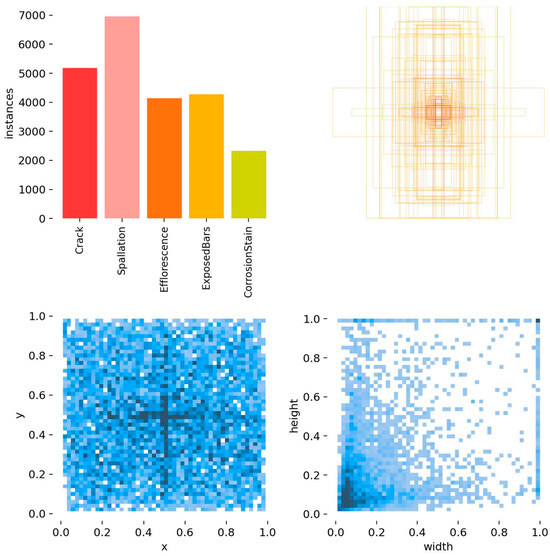
Figure 8.
Visualization of labeled data for each type of disease.
4.2. Data Training
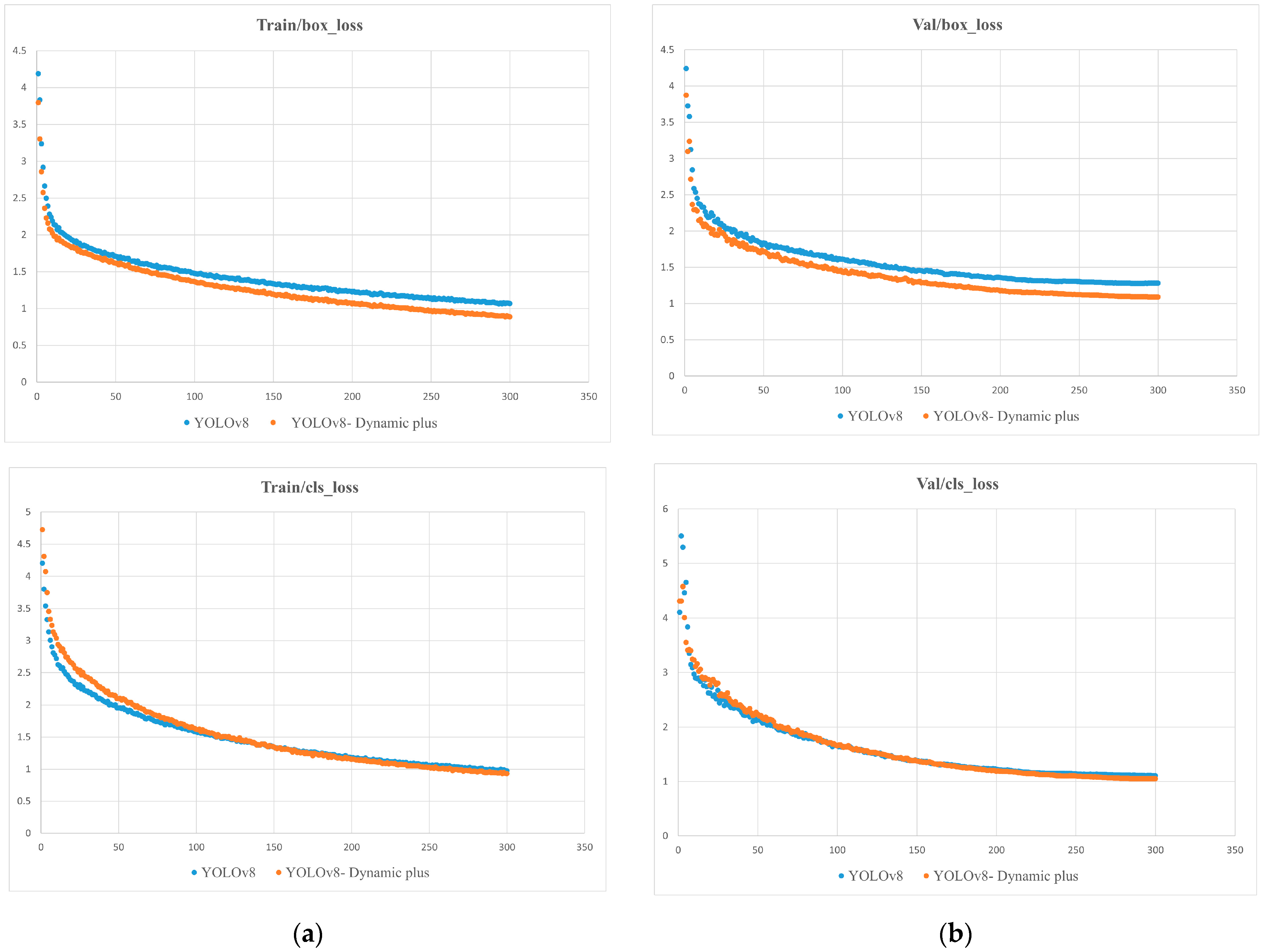
In this study, we used the migration learning method [16] to load the weights of the pretrained model, which can improve the convergence speed when the network model is trained. Input training samples and the disease image training samples were randomly divided into training sets and test sets with a ratio of 9:1, and 10% of the training set was extracted as the validation set. The experiments showed that when the network was in the initial period, the loss value decreased more quickly, and then tended to stabilize, so we chose to use 300 rounds of data training. Specific types of loss curves are shown in Figure 9.
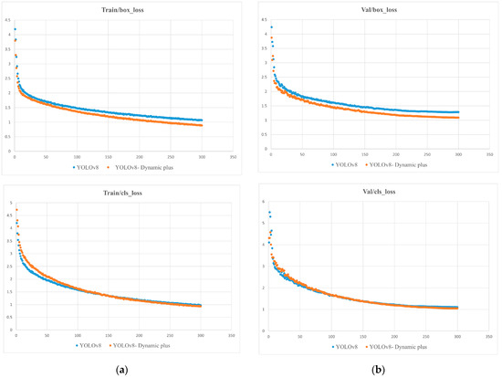
Figure 9.
Comparison of YOLOv8 Dynamic Plus and YOLOv8 loss function curves: (a) Localization loss curves and classification loss curves in the training set; (b) verification of centralized localization loss curves and classification loss curves.
From Figure 9a, it can be observed that in the training set, the optimized box_loss discrete plot is closer to the X-axis, indicating that the predicted box is closer to the real box after the improvement. The cls_loss performance of the improved YOLOv8 Dynamic Plus model is closer to the X-axis after 100 rounds, which reflects the model’s learning of quasi-measurement to predict the location, size, and classification of the disease from the enhanced input image to size and classify and attain faster convergence upon the optimal solution, speeding up convergence and learning efficiency. From Figure 9b, the curves show similar decreasing trends, indicating that the model also shows better generalization ability on new data.
In machine learning and deep learning, the training parameters and hyperparameters of a model have a significant impact on the performance of the model. The parameters and their selection are discussed in detail below.
- (1)
- Input Image Size. The size of the input image determines the amount of image information processed by the model in each training step. The choice of image size directly affects the input layer of the model and the complexity of subsequent feature extraction. If the image is too small, it may lead to loss of information. If it is too large, it may lead to excessive computational cost and memory usage: 640 × 640 is a common choice, balancing detail and computational requirements in many tasks.
- (2)
- Optimizer. The choice of different optimizers affects the speed of convergence and the final performance of the model. SGD is one of the most basic optimization algorithms, and is simple and easy to implement. Although there are many more complex optimization algorithms (e.g., Adam, RMSprop, etc.), SGD is still preferred for many standard tasks due to its stability and simplicity.
- (3)
- Momentum Factor. The momentum factor is a strategy used to accelerate the convergence of SGD by weighting the historical information of the gradient to help the optimizer jump out in local minima. A momentum factor that is too small may lead to convergence that is too slow, and if it is too large, it may introduce oscillations: 0.8 is a common choice and usually provides stable convergence performance.
- (4)
- Number of Freezes. A freeze layer is a network layer that remains unchanged during training and is usually used in migration learning to avoid modifications to the feature extraction part of the pretrained model. The number of frozen layers directly affects the training speed and effectiveness of the model. Too many frozen layers may result in the model not being able to adapt to new tasks. Experimentally, it was shown that 100 frozen layers can retain most of the feature extraction ability of the pre-trained network.
- (5)
- Batch Size. The batch size determines the number of samples used in each gradient update. Larger batches usually increase the training speed, but also require more memory, while smaller batches may result in a noisier and more unstable training process. The experimentally chosen batch sizes of 16 and 8 were chosen as a balance under the computational resource constraints.
- (6)
- Learning Rate. The learning rate controls the step size of each gradient update. Too high a learning rate can lead to unstable training, while too low a learning rate can lead to slower convergence: 0.001 is a common starting value that needs to be adjusted for the learning rate to find the optimal value.
- (7)
- Number of Defrosts. Thaw counts usually refer to the gradual thawing of frozen layers during training for more detailed training. The unfreezing strategy can significantly affect the training effectiveness of the model, and unfreezing too early or too late may lead to poor training results. After experiments, it was found that 200 unfreezes can help the model gradually adapt to new tasks while retaining the original features.
- (8)
- Total Cycles. The total number of training cycles determines the number of model training cycles. Too few training cycles may lead to under-training of the model, while too many may lead to overfitting.
The selection of these parameters usually needs to rely on three considerations: the characteristics of the dataset, the computational resources, and the model architecture. Combining the experimental objectives, dataset characteristics, and computational resources, the network training parameters selected in this study are shown in Table 2.
Table 2.
Initialization of parameters.
4.3. Evaluation Indicators
The evaluation indexes used in this study were precision, recall [17], average precision (AP) [18], and mean average precision (mAP) [19] for each type of disease, with the following equations:
where is predicted to be a positive sample and is actually a positive sample, is predicted to be a positive sample and is actually a negative sample, is predicted to be a negative sample and is actually a positive sample, and denotes the number of disease categories, with the number of categories in this study being 5.
5. Experimental Results and Analysis
5.1. Ablation Experiment
The mAP@0.5 metric was used to measure the model performance in the target detection task, which is calculated by averaging the average precision for each category and then averaging the values when the IoU threshold is 0.5. mAP@0.5 can reflect the model’s detection precision and recall ability comprehensively, with the value ranging from 0 to 1, and a higher value indicates better model performance. The performance of the basic algorithm of this study and other mainstream algorithms were compared, and the results are shown in Table 3. For ease of observation, mAP@0.5 in all data tables are percentages.
Table 3.
The dominant algorithm.
As can be seen from Table 3, comparing the Faster R-CNN and SSD models, although the Faster R-CNN performs better in terms of accuracy, its higher computational complexity leads to slower speeds in real-time detection tasks, making it difficult to satisfy the demand for fast responses. The SSD model, on the other hand, performs well in terms of speed, but its detection accuracy tends to be inferior to that of the Faster R-CNN when dealing with complex scenarios. For the YOLO series, the model selected in this study has the highest accuracy on the CODEBRIM dataset, and although the detection time is not the best among all the models, the difference is not too big, and the YOLOv8 model still performs better under comprehensive consideration. To verify the feasibility of the three improved network structures proposed in this study and the proposed YOLOv8 Dynamic Plus model, ablation experiments were conducted and are described in this section. The experimental training consisted of eight experiments on the four improved networks of YOLOv8, C2f-DWR-DRB(C2fDD), TADDH, and P2. The specific experimental results are shown in Table 4.
Table 4.
Comparisons of the experimental results between various improved networks and the original YOLOv8 network.
In Table 4, it can be seen that for the detection of diseases with insignificant spalling and weathering characteristics in the base network, the accuracy increases by 1.5 and 2 percentage points through the improvement of the C2f module. For diseases with complex backgrounds and large disease areas, the accuracy of cracking and corrosion is increased by 3.6 and 6.3 percentage points through the reconstruction of the TADDH structure. Also, for the small spalling, weathering, and exposed tendon target lesions, the accuracies are improved by 4.9, 4.1, and 3.5 percentage points, respectively, by adding the P2 layer. The experimental results of these three improvements illustrate that utilizing these improvement strategies can help to improve the detection capability and accuracy of the bridge disease detection system for diseases in small targets and complex scenarios and further enhance the accuracy of the network for boundary regression, making it more reliable and effective in practical applications.
In addition, the YOLOv8 Dynamic Plus network model is optimal for all five disease detections, which are improved by 5.2, 8.5, 8.8, 7.8 and 6.6 percentage points, respectively, compared with the original YOLOv8 model. The final mAP@0.5 indicator improved by 7.4 percentage points. The feasibility and effectiveness of the proposed network structure model YOLOv8 Dynamic Plus is demonstrated.
When evaluating model performance, relying only on a single performance metric may not fully reflect the actual performance of the model. To provide a more comprehensive analysis, we combine F1_confidence curves and precision–confidence curves with confidence intervals and p-values for statistical analysis to delve deeper into the significance of the model performance before and after improvement.
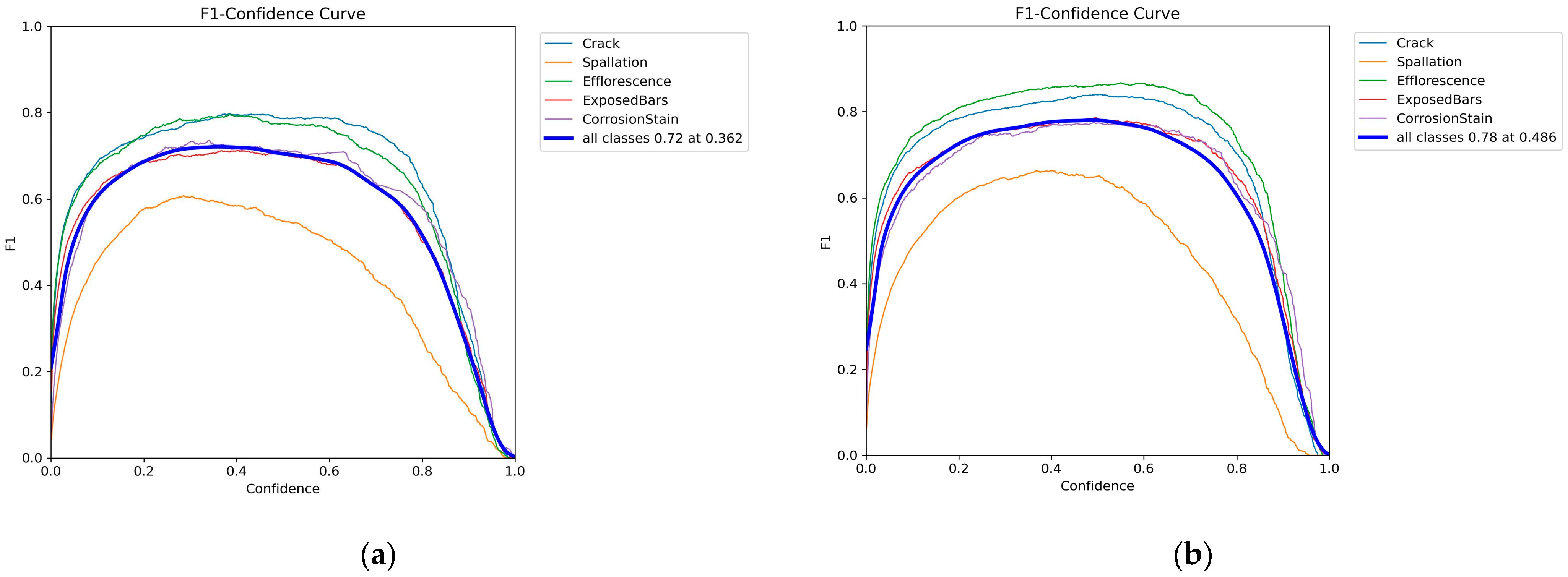
The F1_confidence curve shows the changes in F1 scores under different confidence thresholds, which are the reconciled averages of precision and recall and can effectively measure the overall performance of the classification model in the case of category imbalance. A comparison of the F1–confidence curves before and after model improvement are shown in Figure 10.
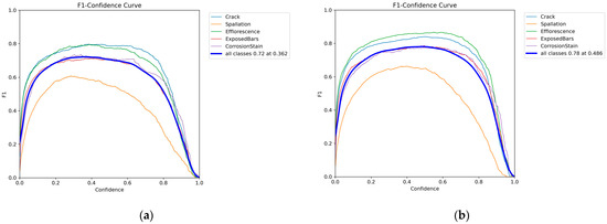
Figure 10.
F1–confidence curves for five types of bridge disease: (a) YOLOv8 model; (b) YOLOv8 Dynamic Plus model.
In the F1–confidence curves, it can be seen that the F1 score shows a tendency to increase and then decrease as the confidence threshold increases. The overall curves of the improved YOLOv8 Dynamic Plus model are all improved compared with the YOLOv8 model before improvement. The results show that the comprehensive performance of the model is enhanced under different confidence thresholds. Specifically, this means that the improved model can provide higher F1 scores at the same confidence level, i.e., both the precision and recall of the model are optimized over a wider range.
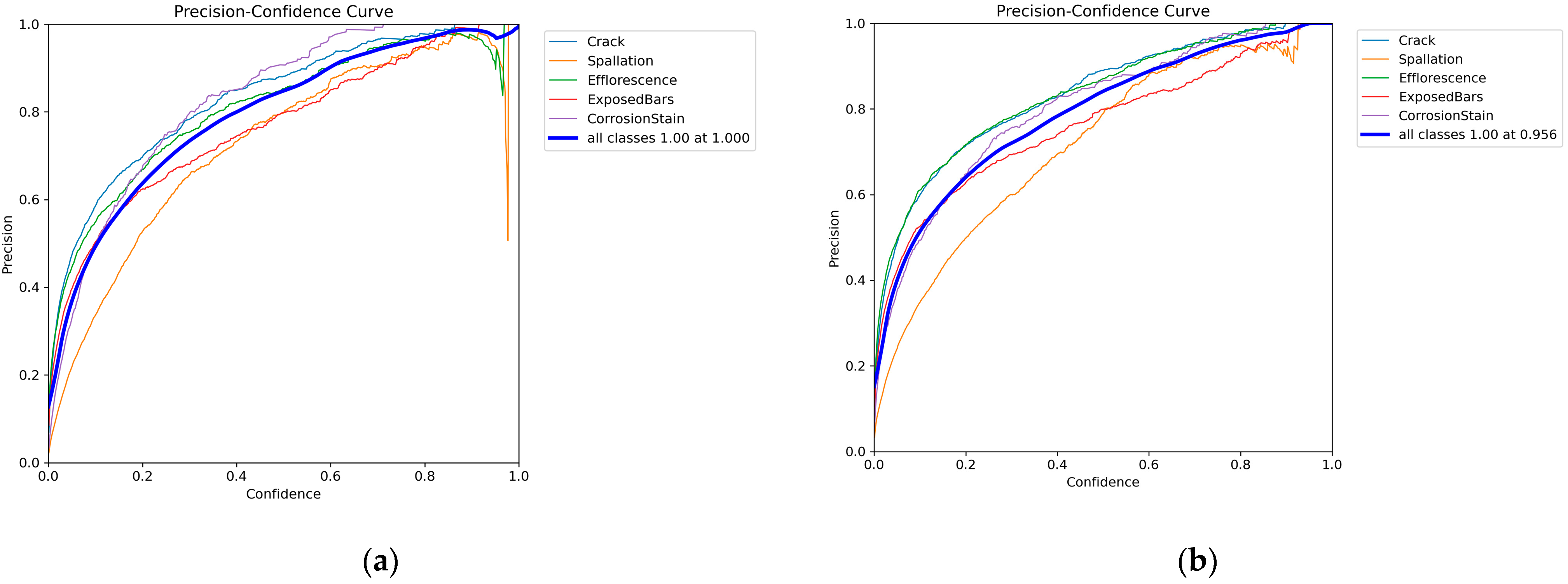
The precision–confidence curves show the changes in the precision rates at different confidence levels. Precision–confidence curves measure the proportions of the samples predicted by the model to be in the positive category that are actually in the positive category. A comparison of the precision–confidence curves before and after model improvement is shown in Figure 11.
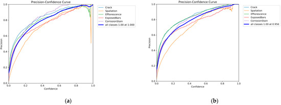
Figure 11.
Precision–confidence curves for five types of bridge disease: (a) YOLOv8 model; (b) YOLOv8 Dynamic Plus model.
As can be seen from the comparison of the precision–confidence curves in Figure 11, for the improved YOLOv8 Dynamic Plus model, the precision values are more convergent in the confidence intervals of 0.4–1.0, and particularly for diseases such as spalling, they do not show any oscillation in the precision values after the improvement that occurred before the improvement at the confidence level of 0.9. The experimental results illustrate that the YOLOv8 Dynamic Plus model significantly improved in terms of consistency and stability of accuracy compared to the pre-improvement period, and in particular performed more reliably when dealing with specific diseases, which indicates that the improvement measures effectively enhanced the performance of the model.
The improved YOLOv8 Dynamic Plus model showed higher stability and consistency in F1–confidence curves and precision–confidence curves through the combined analysis of F1–confidence curves and precision–confidence curves. For bridge distress (e.g., spallation), the model shows a significant improvement in identifying and detecting such distress. This enhancement is particularly important, because it reduces the likelihood of false alarms and omissions and improves the detection efficiency in practical applications. Statistical analysis incorporating confidence intervals and p-values further validated the significance of the improved model performance. These statistical results ensure that the observed performance enhancement is not coincidental, but has substantial statistical support. It enhances the validity of the results and also provides strong support for the optimization and application of concrete building inspection models in the future.
5.2. Experimental Visualization Results
The experimental results of the original model in Table 4 and the YOLOv8 Dynamic Plus model proposed in this study were visualized and compared, and the comparisons are shown in Figure 12.
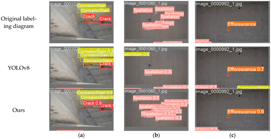
Figure 12.
Comparisons of the visualization results between YOLOv8 Dynamic Plus and YOLOv8: (a) comparison chart for misdetection; (b) comparison chart for leakage detection; (c) comparison chart for detection accuracy.
In Figure 12, we can see that the YOLOv8 Dynamic Plus model proposed in this study has a lower false-detection rate and lower leakage rate than the original YOLOv8 network, while the detection accuracy is higher than the original YOLOv8 network. This shows that the proposed network model can identify small lesions in bridge structures more accurately and reduce the missed detection rate. Small-target bridge diseases may be ignored or misjudged in daily inspection, but they are potential threats to the long-term safety of bridge structures. The improved model can more reliably locate and analyze distress and provide timely and accurate repair recommendations, which can help extend the service life of bridges and reduce maintenance costs.
6. Conclusions
The YOLOv8 Dynamic Plus model proposed in this study effectively reduces the risk of leakage and misdetection in bridge disease detection through the application of structural reparameterization and parallel small-kernel expansion convolution. The newly designed TADDH structure optimizes the consistency prediction of the localization and classification tasks, and is capable of dynamically selecting the interaction information. Also, the added small-target recognition layer significantly enhances the ability to recognizing complex backgrounds and small-target diseases. The overall accuracy of disease detection was improved by optimizing the model architecture, enhancing feature extraction power, and data enhancement techniques. The experimental results show that the accuracy and precision of the model are significantly improved in multiple types of disease detection, which verifies the effectiveness of the proposed model in bridge disease detection. The proposed model provides accurate detection data for the subsequent decision-making process of experts in evaluating the safety of bridges.
Future research should concentrate on refining the confidence scoring strategy of the model. Specifically, efforts should be directed toward mitigating the reduction in recall rates at higher confidence levels while simultaneously improving precision. Advancing the model to support rapid detection of bridge defects will be a critical focus. This involves exploring methods to enhance processing speed without compromising detection accuracy, which is essential for real-time applications. Integrating real-time data acquisition and analysis systems could provide substantial benefits, enabling quicker and more effective identification of structural issues. The next steps will involve optimizing confidence thresholds and developing techniques for swift and reliable detection, which will significantly contribute to the field of structural health monitoring and bridge maintenance.
Author Contributions
Conceptualization, J.G.; methodology, Y.P.; validation, Y.P and J.Z.; data curation, Y.P.; writing—original draft preparation, Y.P.; writing—review and editing, J.G. and Y.P.; software, J.Z. All authors have read and agreed to the published version of the manuscript.
Funding
This research was funded by the Shaanxi Provincial Key Research and Development Program (grant 2020SF-370).
Data Availability Statement
No new data were created or analyzed in this study. Data sharing is not applicable to this article.
Conflicts of Interest
The authors declare no conflicts of interest.
Nomenclature
| Term | Definition |
| Adaptive Layer Attention Network | A network structure that improves a model’s responsiveness to specific features by dynamically adjusting attention layer weights. |
| Attention Mechanism | A technique that enhances a model’s focus on important information by weighting features dynamically. |
| Convolutional Neural Network (CNN) | A deep learning network structure widely used for image and video analysis tasks through convolution operations. |
| C2f Module | An improved convolution module that enhances large-kernel convolution using parallel expansion convolution and structural reparameterization techniques. |
| Deep Learning | A machine learning method that uses neural networks to model and learn from complex patterns in data. |
| Digital Image Processing Technology | A technique that uses computers to process and analyze image data. |
| Graph Convolutional Network (GCN) | A neural network structure used for processing graph data that learns features through node neighborhood information. |
| Image Segmentation | The process of dividing an image into multiple parts or regions for better analysis and processing. |
| You Only Look Once | A real-time target detection algorithm that transforms the target detection problem into a regression problem. |
| YOLOv8 | The latest version of the “You Only Look Once” object detection model. |
| Manual Detection | A traditional bridge inspection method, usually observed and recorded by technicians on-site, is subjective, slow, and has a high leakage rate. |
| Non-Maximum Suppression (NMS) | A technique used to remove redundant detection boxes to retain the best detection results. |
| Region Proposal Network (RPN) | A network component that generates candidate regions for object detection. |
| Small Object Detection Layer | A feature recognition layer specialized for small-target detection. |
| Soft-NMS | An improved version of non-maximum suppression that reduces the scores of overlapping detection boxes instead of removing them outright. |
| Task Align Dynamic Detection Head | A structure for aligning predictions for classification and localization tasks to maintain consistency between them. |
References
- Yao, W.; Jin, X.; Wang, Y. Analysis of urban bridge cluster disease and inspection behavior based on intelligent management system. World Bridge 2023, 51, 115–121. [Google Scholar]
- Peng, W.; Shen, J.; Tang, X.; Zhang, Y. Review, analysis and insights of recent typical concrete construction accidents. China J. Highw. 2019, 32, 132–144. [Google Scholar]
- He, S.; Zhao, X.; Ma, J.; Zhao, Y.; Song, H.; Song, H.; Cheng, L.; Yuan, Z.; Huang, F.; Zhang, J.; et al. A review of highway concrete building inspection and evaluation techniques. China J. Highw. 2017, 30, 63–80. [Google Scholar]
- Lu, M. Study on disease analysis and reinforcement of concrete bridges. Eng. Constr. Des. 2021, 12, 157. [Google Scholar]
- Lin, Z. Current research status of UAV bridge inspection technology. Heilongjiang Transp. Technol. 2023, 46, 61–63. [Google Scholar]
- Gao, J.X. Research on New Technology of Concrete Building Inspection Based on Image Processing and Machine Learning. Master’s Thesis, Southeast University, Nanjing, China, 2018. [Google Scholar]
- Jahanshahi, M.R.; Masri, S.F. Adaptive vision-based crack detection using 3D scene reconstruction for condition assessment of structures. Autom. Constr. 2012, 22, 567–576. [Google Scholar] [CrossRef]
- Hoskere, V.; Narazaki, Y.; Hoang, T.; Spencer, B., Jr. Vision-based structural inspection using multiscale deep convolutional neural networks. arXiv 2018, arXiv:1805.01055. [Google Scholar]
- Song, W. Research on Recognition and Classification of Concrete Building Diseases Based on Image Deep Learning. Master’s Thesis, Beijing University of Posts and Telecommunications, Beijing, China, 2020. [Google Scholar]
- Mu, Z.; Qin, Y.; Yu, C.; Wu, Y.; Wang, Z.; Yang, H.; Huang, Y. Adaptive cropping shallow attention network for defect detection of bridge girder steel using unmanned aerial vehicle images. J. Zhejiang Univ. Sci. A 2023, 24, 243–256. [Google Scholar] [CrossRef]
- Ahmadi, M.; Ebadi-Jamkhaneh, M.; Dalvand, A.; Rezazadeh Eidgahee, D. Hybrid bio-inspired metaheuristic approach for design compressive strength of high-strength concrete-filled high-strength steel tube columns. Neural Comput. Appl. 2024, 36, 7953–7969. [Google Scholar] [CrossRef]
- Chen, H.; Yang, J.; Chen, X.; Zhang, D.; Gan, V.J. Tempnet: A graph convolutional network for temperature field prediction of fire-damaged concrete. Expert Syst. Appl. 2024, 238 Pt B, 121997. [Google Scholar] [CrossRef]
- Redmon, J.; Divvala, S.K.; Girshick, R.B.; Farhadi, A. You only look once: Unified, real-time object detection. In Proceedings of the 2016 IEEE Conference on Computer Vision and Pattern Recognition (CVPR), Las Vegas, NV, USA, 27–30 June 2016. [Google Scholar]
- Zhang, S.H.; Yang, H.K.; Yang, C.H.; Yuan, W.; Li, X.; Wang, X.; Zhang, Y.; Cai, X.; Sheng, Y.; Deng, X.; et al. Edge device detection of tea leaves with one bud and two leaves based on ShuffleNetv2-YOLOv5-Lite-E. Agronomy 2023, 13, 577. [Google Scholar] [CrossRef]
- Loffe, S.; Szegedy, C. Batch normalization: Accelerating deep network training by reducing internal covariate shift. In Proceedings of the 32nd International Conference on Machine Learning (ICML 2015), Lille, France, 6–11 July 2015; pp. 448–456. [Google Scholar]
- Pan, S.J.; Yang, Q. A survey on transfer learning. IEEE Trans. Knowl. Data Eng. 2010, 22, 1345–1359. [Google Scholar] [CrossRef]
- Davis, J.; Goadrich, M. The relationship between Precision-Recall and ROC curves. In Proceedings of the 23rd international conference on Machine learning (ICML), Pittsburgh, PA, USA, 25–29 June 2006; pp. 233–240. [Google Scholar] [CrossRef]
- Everingham, M.; Gool, L.; Williams, C.K.I.; Winn, J.; Zisserman, A. The PASCAL Visual Object Classes (VOC) Challenge. Int. J. Comput. Vis. IJCV 2010, 88, 303–338. [Google Scholar] [CrossRef]
- Girshick, R.B. Fast R-CNN. In Proceedings of the IEEE International Conference on Computer Vision (ICCV), Santiago, Chile, 7–13 December 2015; pp. 1440–1448. [Google Scholar] [CrossRef]


Disclaimer/Publisher’s Note: The statements, opinions and data contained in all publications are solely those of the individual author(s) and contributor(s) and not of MDPI and/or the editor(s). MDPI and/or the editor(s) disclaim responsibility for any injury to people or property resulting from any ideas, methods, instructions or products referred to in the content. |
© 2024 by the authors. Licensee MDPI, Basel, Switzerland. This article is an open access article distributed under the terms and conditions of the Creative Commons Attribution (CC BY) license (https://creativecommons.org/licenses/by/4.0/).