
Exploring Urban Heat Distribution via Intra- and Extra-Block Morphologies with Integrated Stacked Models


Abstract
:1. Introduction
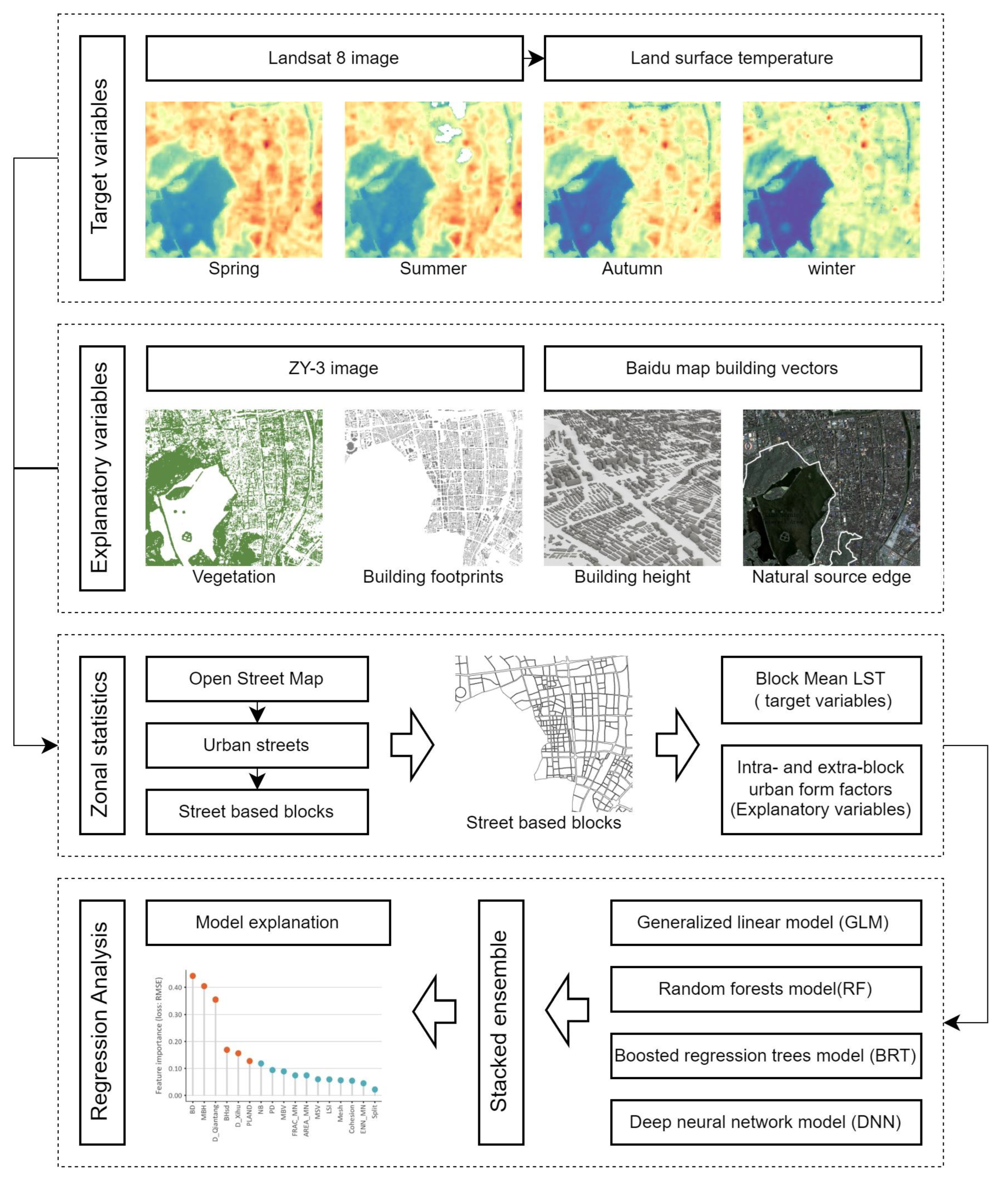
2. Data and Methods
2.1. Study Area
2.2. Data and Preprocessing
2.2.1. Land Surface Temperature
2.2.2. Urban Morphology Data
2.2.3. Computation of Urban Morphological Factors
2.3. Statistical Analysis
2.3.1. Multicollinearity Detection
2.3.2. Stacked Ensemble Models
2.3.3. Model Interpretation
3. Results
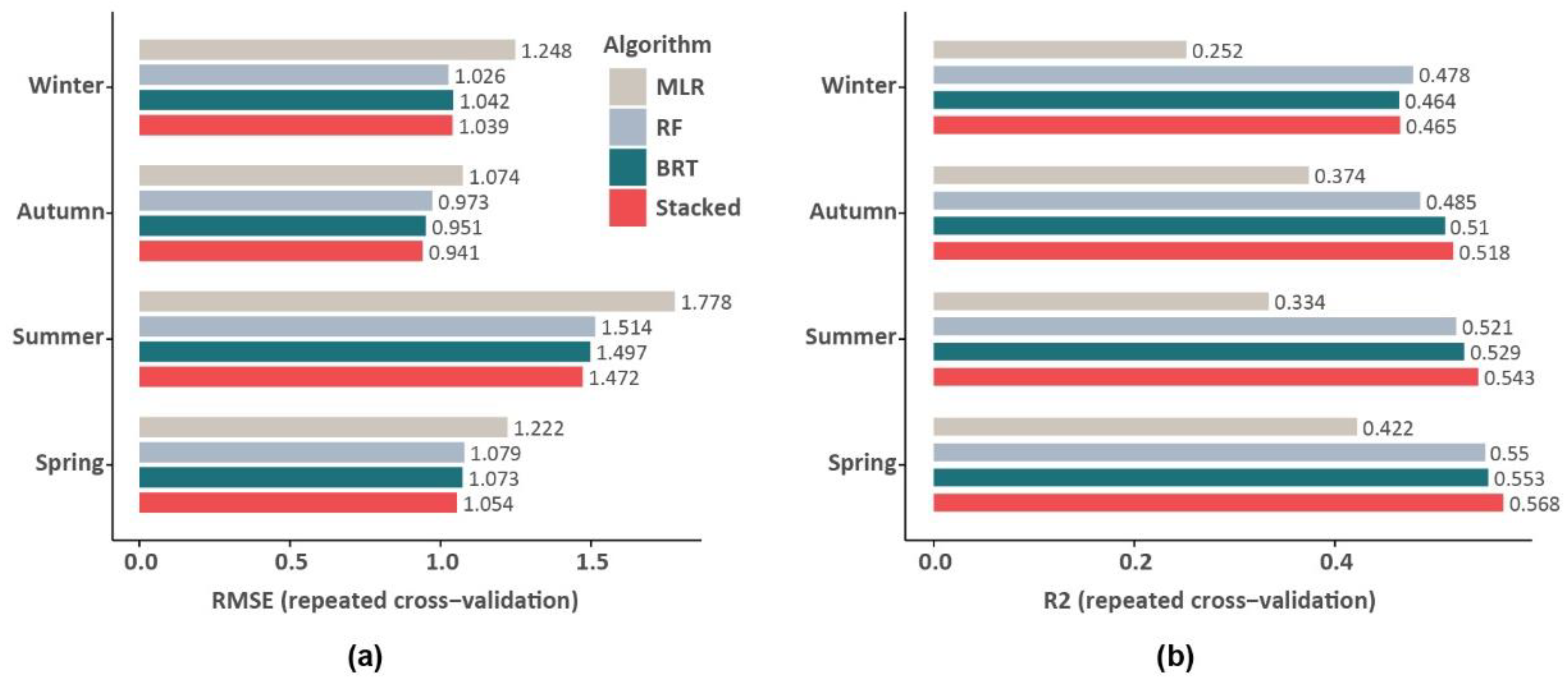
3.1. Model Performance Comparison
3.2. Variable Importance Ranking
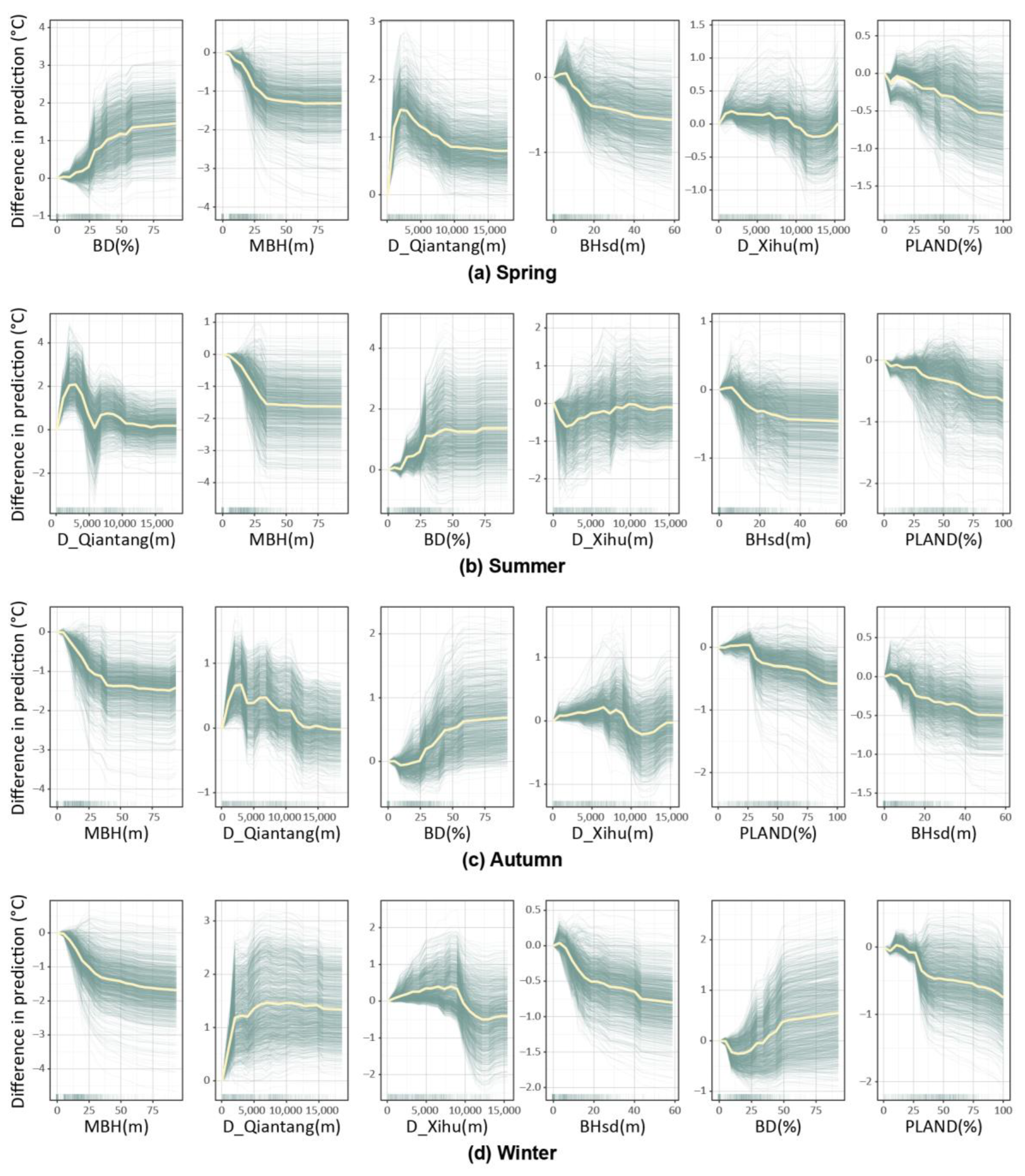
3.3. Correlation Patterns
4. Discussion
4.1. Relative Importance of Urban Morphological Factors to LST
4.2. Vegetation and 3DBF
4.3. External Cold Sources
4.4. Implications for Urban Planning and Management
4.5. Limitations and Future Research
5. Conclusions
Author Contributions
Funding
Data Availability Statement
Acknowledgments
Conflicts of Interest
Appendix A

| Abbreviation | Meaning |
|---|---|
| 3DBF | Three-Dimensional Building Factors |
| ANN | Artificial Neural Networks |
| BRT | Boosted Regression Trees |
| DNN | Deep Neural Networks |
| ECS | External Cold Sources |
| GLM | Generalized Linear Model |
| ICE | Individual Conditional Expectation |
| LST | Land Surface Temperature |
| MLR | Multiple Linear Regression |
| NDBI | Normalized Difference Built-Up Index |
| NDVI | Normalized Difference Vegetation Index |
| PDP | Partial Dependence Plots |
| RF | Random Forest |
| RMSE | Root Mean Square Error |
| R2 | Coefficient of Determination |
| UGS | Urban Green Spaces |
| UHI | Urban Heat Island |
| Variables | Coefficients before the VIF Test | Original VIF | Coefficients after the VIF Test | Final VIF | ||||||
|---|---|---|---|---|---|---|---|---|---|---|
| Spring | Summer | Autumn | Winter | Spring | Summer | Autumn | Winter | |||
| AI | (−)0.0092 | 0.0122 | (−)0.0038 | (−)0.0207 * | 11.1281 | - | - | - | - | - |
| AREA_MN | (−)0.0191 | (−)0.0915 | (−)0.0326 | (−)0.0160 | 2.9037 | 0.0509 | (−)0.0696 | 0.0815 | 0.2232 *** | 2.1061 |
| Cohesion | 0.0232 * | 0.0016 | 0.0176 * | 0.0463 *** | 9.8173 | 0.0098 | 0.0201 | 0.0082 | 0.0269 *** | 3.3942 |
| Division | (−)0.7793 | (−)1.1668 | 0.0018 | 0.3477 | 22.2067 | - | - | - | - | |
| ED | (−)0.0009 | 0.0001 | (−)0.0018 *** | (−)0.0030 *** | 6.6587 | - | - | - | - | |
| ENN_MN | (−)0.0080 * | (−)0.0066 | (−)0.0089 *** | (−)0.0061 * | 1.3719 | (−)0.0057 | (−)0.0123 | (−)0.0086 ** | (−)0.0083 * | 1.3648 |
| FRAC_MN | (−)3.3740 ** | (−)4.1997 * | (−)0.5529 | 0.2785 | 2.1164 | (−)3.8464 *** | (−)5.6991 *** | (−)3.5650 *** | (−)4.321 *** | 1.3959 |
| LPI | (−)0.0114 | (−)0.010 | (−)0.0061 | (−)0.0113 | 29.5839 | - | - | - | - | - |
| LSI | 0.0244 | 0.0417 | 0.0117 | (−)0.0146 | 3.1616 | 0.0456 * | 0.0224 | (−)0.0086 | (−)0.0408 * | 1.8160 |
| Mesh | (−)0.0387 ** | (−)0.0430 * | (−)0.0231 * | (−)0.0120 | 2.3831 | (−)0.0438 *** | (−)0.0413 * | (−)3.5650 | (−)0.014 | 2.0135 |
| PD | 0.0003 | (−)0.0010 | 0.0001 | 0.0006 | 3.7570 | <0.001 | (−)0.0006 | (−)0.0005 | (−)0.0009 ** | 1.9921 |
| PLAND | (−)0.004 | (−)0.0213 * | 0.0019 | 0.0187 ** | 19.0260 | (−)0.0147 *** | (−)0.0217 *** | (−)0.0180 *** | (−)0.0230 *** | 3.5693 |
| Split | (−)<0.001 | (−)<0.001 | <0.001 | <0.001 | 1.6803 | (−)<0.001 | <0.001 | <0.001 | <0.001 | 1.5436 |
| BD | 0.0353 *** | 0.0416 *** | 0.0231 *** | 0.0252 *** | 3.3974 | 0.0383 *** | 0.0375 *** | 0.0138 *** | 0.0138 ** | 2.8642 |
| MBH | (−)0.0268 *** | (−)0.0255 *** | (−)0.0193 *** | (−)0.0160 *** | 4.2622 | (−)0.0299 *** | (−)0.0329 *** | (−)0.0332 *** | (−)0.0297 *** | 3.4217 |
| BHsd | (−)0.031 *** | (−)0.0305 *** | (−)0.0310 *** | (−)0.0365 *** | 2.8377 | (−)0.0301 *** | (−)0.0285 *** | (−)0.0282 *** | (−)0.0350 *** | 2.7955 |
| MBV | <0.001 | <0.001 | <0.001 | <0.001 | 1.9158 | <0.001 | <0.001 * | <0.001 | <0.001 | 1.8461 |
| MSV | 0.3716 | (−)0.1302 | 0.0766 | 0.2758 | 1.1755 | 0.4072 | (−)0.0456 | 0.1029 | 0.4100 | 1.1555 |
| NB | 0.0005 * | 0.0003 | 0.0012 *** | 0.0008 *** | 4.5248 | <0.001 | 0.0002 | 0.0002 | 0.0001 | 2.6480 |
| SVF | 0.6278 | 0.8733 | 3.2521 *** | 3.6940 *** | 6.5688 | - | - | - | - | - |
| D_Xihu | (−)<0.001 ** | <0.001 *** | (−)<0.001 ** | (−)<0.001 *** | 1.3855 | (−)<0.001 * | <0.001 *** | (−)<0.001 | (−)<0.001 ** | 1.3673 |
| D_Qiantang | (−)<0.001 *** | (−)0.0001 *** | (−)<0.001 *** | <0.001 *** | 1.2796 | (−)<0.001 *** | (−)0.0001 *** | (−)<0.001 *** | <0.001 *** | 1.2643 |
| Model | Hyperparameters |
|---|---|
| MLR | Not applicable; |
| GLM | Alpha: 0.1; |
| RF | Mtry: 3 to 15 with intervals of 3; Ntree: 300 to 1500 with intervals of 300; Node size: 2 to 10 with intervals of 2; |
| BRT | Tree depth: 3 to 12 with intervals of 3; Tree number: 100 to 1000 with intervals of 100; Learning rate: 0.1 to 0.3 with intervals of 0.1; Minimum number of observations required: 5 to 15 with intervals of 5; |
| DNN | Batch size: 200 to 1000 with intervals of 200; Learning rate: 0.02 to 0.1 with intervals of 0.02; Epochs: 20 to 100 with intervals of 20; Neurons per layer: 10 to 100 with intervals of 10; |
| Stacked ensemble | Ensembles the above four models (GLM, RF, BRT, and DNN) using the same grid-search hyperparameters, then applies a GLM for meta-analysis. |
References
- Oke, T.R. The energetic basis of the urban heat island. Q. J. R. Meteorol. Soc. 1982, 108, 1–24. [Google Scholar] [CrossRef]
- Ho, J.Y.; Shi, Y.; Lau, K.K.L.; Ng, E.Y.Y.; Ren, C.; Goggins, W.B. Urban heat island effect-related mortality under extreme heat and non-extreme heat scenarios: A 2010–2019 case study in Hong Kong. Sci. Total Environ. 2023, 858, 159791. [Google Scholar] [CrossRef] [PubMed]
- Masson-Delmotte, V.; Zhai, P.; Pirani, A.; Connors, S.L.; Péan, C.; Berger, S.; Caud, N.; Chen, Y.; Goldfarb, L.; Gomis, M.I. Climate change 2021: The physical science basis. In Contribution of Working Group I to the Sixth Assessment Report of the Intergovernmental Panel on Climate Change; Cambridge University Press: Cambridge, UK; New York, NY, USA, 2021; p. 2. [Google Scholar] [CrossRef]
- Santamouris, M.; Cartalis, C.; Synnefa, A.; Kolokotsa, D. On the impact of urban heat island and global warming on the power demand and electricity consumption of buildings—A review. Energy Build. 2015, 98, 119–124. [Google Scholar] [CrossRef]
- Manoli, G.; Fatichi, S.; Schläpfer, M.; Yu, K.; Crowther, T.W.; Meili, N.; Burlando, P.; Katul, G.G.; Bou-Zeid, E. Magnitude of urban heat islands largely explained by climate and population. Nature 2019, 573, 55–60. [Google Scholar] [CrossRef] [PubMed]
- Nejat, P.; Jomehzadeh, F.; Taheri, M.M.; Gohari, M.; Abd Majid, M.Z. A global review of energy consumption, CO2 emissions and policy in the residential sector (with an overview of the top ten CO2 emitting countries). Renew. Sustain. Energy Rev. 2015, 43, 843–862. [Google Scholar] [CrossRef]
- Logan, T.M.; Zaitchik, B.; Guikema, S.; Nisbet, A. Night and day: The influence and relative importance of urban characteristics on remotely sensed land surface temperature. Remote Sens. Environ. 2020, 247, 111861. [Google Scholar] [CrossRef]
- Battista, G.; Evangelisti, L.; Guattari, C.; De Cristo, E.; De Lieto Vollaro, R.; Asdrubali, F. An Extensive Study of the Urban Heat Island Phenomenon in Rome, Italy: Implications for Building Energy Performance through Data from Multiple Meteorological Stations. Int. J. Sustain. Dev. Plan. 2023, 18, 3357–3362. [Google Scholar] [CrossRef]
- Li, Y.; Yang, T.; Zhao, G.; Ma, C.; Yan, Y.; Xu, Y.; Wang, L.; Wang, L. A Systematic Review of Studies Involving Canopy Layer Urban Heat Island: Monitoring and Associated Factors. Ecol. Indic. 2024, 158, 111424. [Google Scholar] [CrossRef]
- Cheela, V.R.S.; John, M.; Biswas, W.; Sarker, P. Combating Urban Heat Island Effect—A Review of Reflective Pavements and Tree Shading Strategies. Buildings 2021, 11, 93. [Google Scholar] [CrossRef]
- Eludoyin, O.M.; Adelekan, I.O.; Webster, R.; Eludoyin, A.O. Air temperature, relative humidity, climate regionalization and thermal comfort of Nigeria. Int. J. Climatol. 2014, 34, 2000–2018. [Google Scholar] [CrossRef]
- Scott, A.A.; Zaitchik, B.; Waugh, D.W.; O’Meara, K. Intraurban Temperature Variability in Baltimore. J. Appl. Meteorol. Climatol. 2017, 56, 159–171. [Google Scholar] [CrossRef]
- Peng, J.; Jia, J.; Liu, Y.; Li, H.; Wu, J. Seasonal contrast of the dominant factors for spatial distribution of land surface temperature in urban areas. Remote Sens. Environ. 2018, 215, 255–267. [Google Scholar] [CrossRef]
- Ayanlade, A. Seasonality in the daytime and night-time intensity of land surface temperature in a tropical city area. Sci. Total Environ. 2016, 557–558, 415–424. [Google Scholar] [CrossRef] [PubMed]
- Li, T.; Huang, X.; Guo, H.; Hong, T. Contribution and Marginal Effects of Landscape Patterns on Thermal Environment: A Study Based on the BRT Model. Buildings 2024, 14, 2388. [Google Scholar] [CrossRef]
- Han, D.; An, H.; Wang, F.; Xu, X.; Qiao, Z.; Wang, M.; Sui, X.; Liang, S.; Hou, X.; Cai, H.; et al. Understanding seasonal contributions of urban morphology to thermal environment based on boosted regression tree approach. Build. Environ. 2022, 226, 109770. [Google Scholar] [CrossRef]
- Li, J.; Song, C.; Cao, L.; Zhu, F.; Meng, X.; Wu, J. Impacts of landscape structure on surface urban heat islands: A case study of Shanghai, China. Remote Sens. Environ. 2011, 115, 3249–3263. [Google Scholar] [CrossRef]
- Sun, Y.; Gao, C.; Li, J.; Wang, R.; Liu, J. Quantifying the Effects of Urban Form on Land Surface Temperature in Subtropical High-Density Urban Areas Using Machine Learning. Remote Sens. 2019, 11, 959. [Google Scholar] [CrossRef]
- Yuan, F.; Bauer, M.E. Comparison of impervious surface area and normalized difference vegetation index as indicators of surface urban heat island effects in Landsat imagery. Remote Sens. Environ. 2007, 106, 375–386. [Google Scholar] [CrossRef]
- Zhou, D.; Zhao, S.; Liu, S.; Zhang, L.; Zhu, C. Surface urban heat island in China’s 32 major cities: Spatial patterns and drivers. Remote Sens. Environ. 2014, 152, 51–61. [Google Scholar] [CrossRef]
- Estoque, R.C.; Murayama, Y.; Myint, S.W. Effects of landscape composition and pattern on land surface temperature: An urban heat island study in the megacities of Southeast Asia. Sci. Total Environ. 2017, 577, 349–359. [Google Scholar] [CrossRef]
- Zhou, W.; Qian, Y.; Li, X.; Li, W.-J.; Li, W.; Han, L. Relationships between land cover and the surface urban heat island: Seasonal variability and effects of spatial and thematic resolution of land cover data on predicting land surface temperatures. Landsc. Ecol. 2014, 29, 153–167. [Google Scholar] [CrossRef]
- Chen, A.; Yao, L.; Sun, R.; Chen, L. How many metrics are required to identify the effects of the landscape pattern on land surface temperature. Ecol. Indic. 2014, 45, 424–433. [Google Scholar] [CrossRef]
- Zhou, W.; Wang, J.; Cadenasso, M.L. Effects of the spatial configuration of trees on urban heat mitigation: A comparative study. Remote Sens. Environ. 2017, 195, 1–12. [Google Scholar] [CrossRef]
- Liu, Y.; Liu, Y.; Peng, J.; Wang, Y. Efficiency of landscape metrics characterizing urban land surface temperature. Landsc. Urban Plan. 2018, 180, 36–53. [Google Scholar] [CrossRef]
- Zhou, L.; Hu, F.; Wang, B.; Wei, C.; Sun, D.; Wang, S. Relationship between urban landscape structure and land surface temperature: Spatial hierarchy and interaction effects. Sustain. Cities Soc. 2022, 80, 103795. [Google Scholar] [CrossRef]
- Zeng, P.; Sun, F.; Liu, Y.; Tian, T.; Wu, J.; Dong, Q.; Peng, S.; Che, Y. The influence of the landscape pattern on the urban land surface temperature varies with the ratio of land components: Insights from 2D/3D building/vegetation metrics. Sustain. Cities Soc. 2022, 78, 103599. [Google Scholar] [CrossRef]
- Wu, W.-B.; Yu, Z.-W.; Ma, J.; Zhao, B. Quantifying the influence of 2D and 3D urban morphology on the thermal environment across climatic zones. Landsc. Urban Plan. 2022, 226, 104499. [Google Scholar] [CrossRef]
- Yu, S.; Chen, Z.; Yu, B.; Wang, L.; Wu, B.; Wu, J.; Zhao, F. Exploring the relationship between 2D/3D landscape pattern and land surface temperature based on explainable eXtreme Gradient Boosting tree: A case study of Shanghai, China. Sci. Total Environ. 2020, 725, 138229. [Google Scholar] [CrossRef]
- Yuan, B.; Zhou, L.; Dang, X.; Sun, D.; Hu, F.; Mu, H. Separate and combined effects of 3D building features and urban green space on land surface temperature. J. Environ. Manag. 2021, 295, 113116. [Google Scholar] [CrossRef]
- Wang, Q.; Wang, X.; Zhou, Y.; Liu, D.; Wang, H. The Dominant Factors and Influence of Urban Characteristics on Land Surface Temperature Using Random Forest Algorithm. Sustain. Cities Soc. 2022, 79, 103722. [Google Scholar] [CrossRef]
- Sun, F.; Liu, M.; Wang, Y.; Wang, H.; Che, Y. The effects of 3D architectural patterns on the urban surface temperature at a neighborhood scale: Relative contributions and marginal effects. J. Clean. Prod. 2020, 258, 120706. [Google Scholar] [CrossRef]
- Lu, H.; Li, F.; Yang, G.; Sun, W. Multi-scale impacts of 2D/3D urban building pattern in intra-annual thermal environment of Hangzhou, China. Int. J. Appl. Earth Obs. Geoinf. 2021, 104, 102558. [Google Scholar] [CrossRef]
- Feyisa, G.L.; Dons, K.; Meilby, H. Efficiency of parks in mitigating urban heat island effect: An example from Addis Ababa. Landsc. Urban Plan. 2014, 123, 87–95. [Google Scholar] [CrossRef]
- Peng, J.; Dan, Y.; Qiao, R.; Liu, Y.; Dong, J.; Wu, J. How to quantify the cooling effect of urban parks? Linking maximum and accumulation perspectives. Remote Sens. Environ. 2021, 252, 112135. [Google Scholar] [CrossRef]
- Zhou, Y.; Zhao, H.; Mao, S.; Zhang, G.; Jin, Y.; Luo, Y.; Huo, W.; Pan, Z.; An, P.; Lun, F. Studies on urban park cooling effects and their driving factors in China: Considering 276 cities under different climate zones. Build. Environ. 2022, 222, 109441. [Google Scholar] [CrossRef]
- Cao, B.; Chen, Q.; Du, M.; Cheng, Q.; Li, Y.; Liu, R. Simulation Analysis of the Cooling Effect of Urban Water Bodies on the Local Thermal Environment. Water 2022, 14, 3091. [Google Scholar] [CrossRef]
- Cheng, L.; Guan, D.; Zhou, L.; Zhao, Z.; Zhou, J. Urban cooling island effect of main river on a landscape scale in Chongqing, China. Sustain. Cities Soc. 2019, 47, 101501. [Google Scholar] [CrossRef]
- Zhou, W.; Huang, G.; Cadenasso, M.L. Does spatial configuration matter? Understanding the effects of land cover pattern on land surface temperature in urban landscapes. Landsc. Urban Plan. 2011, 102, 54–63. [Google Scholar] [CrossRef]
- Buyantuyev, A.; Wu, J. Urban heat islands and landscape heterogeneity: Linking spatiotemporal variations in surface temperatures to land-cover and socioeconomic patterns. Landsc. Ecol. 2010, 25, 17–33. [Google Scholar] [CrossRef]
- Guo, F.; Wu, Q.; Schlink, U. 3D building configuration as the driver of diurnal and nocturnal land surface temperatures: Application in Beijing’s old city. Build. Environ. 2021, 206, 108354. [Google Scholar] [CrossRef]
- Li, H.; Li, Y.; Wang, T.; Wang, Z.; Gao, M.; Shen, H. Quantifying 3D building form effects on urban land surface temperature and modeling seasonal correlation patterns. Build. Environ. 2021, 204, 108132. [Google Scholar] [CrossRef]
- Han, D.; An, H.; Cai, H.; Wang, F.; Xu, X.; Qiao, Z.; Jia, K.; Sun, Z.; An, Y. How do 2D/3D urban landscapes impact diurnal land surface temperature: Insights from block scale and machine learning algorithms. Sustain. Cities Soc. 2023, 99, 104933. [Google Scholar] [CrossRef]
- Li, Z.; Hu, D. Exploring the relationship between the 2D/3D architectural morphology and urban land surface temperature based on a boosted regression tree: A case study of Beijing, China. Sustain. Cities Soc. 2022, 78, 103392. [Google Scholar] [CrossRef]
- Lu, L.; Fu, P.; Dewan, A.; Li, Q. Contrasting determinants of land surface temperature in three megacities: Implications to cool tropical metropolitan regions. Sustain. Cities Soc. 2023, 92, 104505. [Google Scholar] [CrossRef]
- Wang, Q.; Wang, X.; Meng, Y.; Zhou, Y.; Wang, H. Exploring the impact of urban features on the spatial variation of land surface temperature within the diurnal cycle. Sustain. Cities Soc. 2023, 91, 104432. [Google Scholar] [CrossRef]
- Al-Rbaihat, R.; Saleh, K.; Malpress, R.; Buttsworth, D.; Alahmer, H.; Alahmer, A. Performance Evaluation of Supersonic Flow for Variable Geometry Radial Ejector through CFD Models Based on DES-Turbulence Models, GPR Machine Learning, and MPA Optimization. Int. J. Thermofluids 2023, 20, 100487. [Google Scholar] [CrossRef]
- Li, Z.; Zhang, C.; Liu, H.; Zhang, C.; Zhao, M.; Gong, Q.; Fu, G. Developing stacking ensemble models for multivariate contamination detection in water distribution systems. Sci. Total Environ. 2022, 828, 154284. [Google Scholar] [CrossRef]
- van der Laan, M.J.; Polley, E.C.; Hubbard, A.E. Super Learner. Stat. Appl. Genet. Mol. Biol. 2007, 6. [Google Scholar] [CrossRef]
- Peel, M.C.; Finlayson, B.L.; McMahon, T.A. Updated world map of the Köppen-Geiger climate classification. Hydrol. Earth Syst. Sci. 2007, 11, 1633–1644. [Google Scholar] [CrossRef]
- Landsat 8–9 Collection 2 Level 2 Science Product Guide | U.S. Geological Survey. (n.d.). Available online: https://www.usgs.gov/media/files/landsat-8-9-collection-2-level-2-science-product-guide (accessed on 24 August 2022).
- Ni, W.; Sun, G.; Ranson, K.J.; Pang, Y.; Zhang, Z.; Yao, W. Extraction of ground surface elevation from ZY-3 winter stereo imagery over deciduous forested areas. Remote Sens. Environ. 2015, 159, 194–202. [Google Scholar] [CrossRef]
- Bhandari, A.K.; Kumar, A.; Singh, G.K. Feature Extraction using Normalized Difference Vegetation Index (NDVI): A Case Study of Jabalpur City. Procedia Technol. 2012, 6, 612–621. [Google Scholar] [CrossRef]
- Chen, D.; Zhang, F.; Zhang, M.; Meng, Q.; Jim, C.Y.; Shi, J.; Tan, M.L.; Ma, X. Landscape and vegetation traits of urban green space can predict local surface temperature. Sci. Total Environ. 2022, 825, 154006. [Google Scholar] [CrossRef] [PubMed]
- Daoud, J.I. Multicollinearity and regression analysis. J. Phys. Conf. Ser. 2017, 949, 012009. [Google Scholar] [CrossRef]
- Nelder, J.A.; Wedderburn, R.W. Generalized linear models. J. R. Stat. Soc. Ser. A (General) 1972, 135, 370–384. [Google Scholar] [CrossRef]
- Breiman, L. Random Forests. Mach. Learn. 2001, 45, 5–32. [Google Scholar] [CrossRef]
- Friedman, J.H. Greedy Function Approximation: A Gradient Boosting Machine. Ann. Stat. 2001, 29, 1189–1232. [Google Scholar] [CrossRef]
- Montavon, G.; Samek, W.; Müller, K.-R. Methods for interpreting and understanding deep neural networks. Digit. Signal Process. 2018, 73, 1–15. [Google Scholar] [CrossRef]
- Trost, J.E. Statistically nonrepresentative stratified sampling: A sampling technique for qualitative studies. Qual. Sociol. 1986, 9, 54–57. [Google Scholar] [CrossRef]
- Refaeilzadeh, P.; Tang, L.; Liu, H. Cross-Valid. Encycl. Database Syst. 2009, 5, 532–538. [Google Scholar]
- Petch, J.; Di, S.; Nelson, W. Opening the Black Box: The Promise and Limitations of Explainable Machine Learning in Cardiology. Can. J. Cardiol. 2022, 38, 204–213. [Google Scholar] [CrossRef]
- Molnar, C. Interpretable machine learning. Lulu. com. 2020. Available online: https://www.amazon.com/Interpretable-Machine-Learning-Making-Explainable/dp/B09TMWHVB4 (accessed on 24 August 2022).
- Yang, C.; Zhu, W.; Sun, J.; Xu, X.; Wang, R.; Lu, Y.; Zhang, S.; Zhou, W. Assessing the effects of 2D/3D urban morphology on the 3D urban thermal environment by using multi-source remote sensing data and UAV measurements: A case study of the snow-climate city of Changchun, China. J. Clean. Prod. 2021, 321, 128956. [Google Scholar] [CrossRef]
- Liu, Y.; Xu, Y.; Weng, F.; Zhang, F.; Shu, W. Impacts of urban spatial layout and scale on local climate: A case study in Beijing. Sustain. Cities Soc. 2021, 68, 102767. [Google Scholar] [CrossRef]
- Stewart, I.D.; Oke, T.R. Local climate zones for urban temperature studies. Bull. Am. Meteorol. Soc. 2012, 93, 1879–1900. [Google Scholar] [CrossRef]
- Qi, J.-D.; He, B.-J.; Wang, M.; Zhu, J.; Fu, W.-C. Do grey infrastructures always elevate urban temperature? No, utilizing grey infrastructures to mitigate urban heat island effects. Sustain. Cities Soc. 2019, 46, 101392. [Google Scholar] [CrossRef]
- Oke, T.R.; Mills, G.; Christen, A.; Voogt, J.A. Urban Climates, 1st ed.; Cambridge University Press: Cambridge, UK, 2017. [Google Scholar] [CrossRef]
- Lai, D.; Liu, W.; Gan, T.; Liu, K.; Chen, Q. A review of mitigating strategies to improve the thermal environment and thermal comfort in urban outdoor spaces. Sci. Total Environ. 2019, 661, 337–353. [Google Scholar] [CrossRef]
- Tan, X.; Sun, X.; Huang, C.; Yuan, Y.; Hou, D. Comparison of cooling effect between green space and water body. Sustain. Cities Soc. 2021, 67, 102711. [Google Scholar] [CrossRef]
- Middel, A.; Lukasczyk, J.; Maciejewski, R.; Demuzere, M.; Roth, M. Sky View Factor footprints for urban climate modeling. Urban Clim. 2018, 25, 120–134. [Google Scholar] [CrossRef]


| Season | Date | Acquisition Time | Path/Row | Cloud Cover (%) | Air Temperature (°C) 1 |
|---|---|---|---|---|---|
| Spring | 15 April 2019 | 10:30 AM | 119/039 | 1.04 | 17.78 |
| Summer | 21 August 2019 | 10:31 AM | 119/039 | 4.58 | 32.22 |
| Autumn | 3 November 2017 | 10:31 AM | 119/039 | 0.07 | 22.22 |
| Winter | 23 February 2018 | 10:31 AM | 119/039 | 4.09 | 7.78 |
| Category | Name | Abbr. | Formula | Paraphrase | Description |
|---|---|---|---|---|---|
| UGS (intra-block) | Mean path area (hectares) | AREA_MN | TA, total projection area of vegetation/building (hectare) 1; N, number of vegetation/building patches 1 | Mean patch area of vegetation | |
| Patch cohesion index (%) | Cohesion | Pi, perimeter of patch i (m); Ai, area of patch i (m2); Z, number of cells | Connectedness (aggregated or isolated) of vegetation patches | ||
| Mean of Euclidean nearest neighbor distance (m) | ENN_MN | hi, distance (m) from patch i to the nearest neighboring patch on the basis of patch edge-to-edge distance | Mean distance of each patch to the nearest neighboring patch | ||
| Mean fractal dimension index (unit: none) | FRAC_MN | - | Mean vegetation patch complexity | ||
| Landscape shape index (units: none) | LSI | Ei, total edge length (m) on cell surfaces; minEi, minimum total edge length (m) on cell surfaces | Ratio between actual edge length and hypothetical minimum edge length | ||
| Effective mesh size (hectares) | Mesh | BA, area of a block (m2) | Relative patch structure | ||
| Patch density (number per km2) | PD | - | Number of vegetation patches per km2 | ||
| Percentage of landscape (%) | PLAND | - | Percentage of the vegetation area | ||
| Splitting index (unit: none) | Split | - | Number of patches if all patches were divided into equally sized patches | ||
| 3DBF (intra-block) | Building density (%) | BD | - | Percentage of building footprints | |
| Mean building height (m) | MBH | Hi, height of building i | Mean building height | ||
| Mean building height standard deviation (m) | BHsd | MH, mean building height in the target block | Variation degree of the heights of buildings | ||
| Mean building volume (m3) | MBV | Vi, volume of building i | Mean building volume | ||
| Mean surface area to volume ratio (m−1) | MSV | SAi, surface area of building i | Mean surface area per unit volume of buildings in the target block; it reflects heat conduction rate | ||
| Number of buildings (number per km2) | NB | - | Number of buildings per km2 | ||
| ECS (extra-block) | Distance to Qiantang River (m) | D_Qiangtang | - | - | Shortest distance from the shape center point of each block to the edge of Qiantang River |
| Distance to Xihu Scenic Interest Area (m) | D_Xihu | - | - | Shortest distance from the shape center point of each block to the edge of Xihu Scenic Interest Area |
| Steps | Packages | Steps |
|---|---|---|
| VIF calculation | car | VIF calculation |
| RF | caret | RF |
| BRT | caret | BRT |
| Stacked ensembles | h2o | Stacked ensembles |
| Stratified sampling | rsample | Stratified sampling |
| Permutation based importance | vip | Permutation based importance |
Disclaimer/Publisher’s Note: The statements, opinions and data contained in all publications are solely those of the individual author(s) and contributor(s) and not of MDPI and/or the editor(s). MDPI and/or the editor(s) disclaim responsibility for any injury to people or property resulting from any ideas, methods, instructions or products referred to in the content. |
© 2024 by the authors. Licensee MDPI, Basel, Switzerland. This article is an open access article distributed under the terms and conditions of the Creative Commons Attribution (CC BY) license (https://creativecommons.org/licenses/by/4.0/).
Share and Cite
Xia, Y.; Wang, Q.; Ren, L.; Wang, H. Exploring Urban Heat Distribution via Intra- and Extra-Block Morphologies with Integrated Stacked Models. Buildings 2024, 14, 3187. https://doi.org/10.3390/buildings14103187
Xia Y, Wang Q, Ren L, Wang H. Exploring Urban Heat Distribution via Intra- and Extra-Block Morphologies with Integrated Stacked Models. Buildings. 2024; 14(10):3187. https://doi.org/10.3390/buildings14103187
Chicago/Turabian StyleXia, Yike, Qi Wang, Lanhong Ren, and Haitao Wang. 2024. "Exploring Urban Heat Distribution via Intra- and Extra-Block Morphologies with Integrated Stacked Models" Buildings 14, no. 10: 3187. https://doi.org/10.3390/buildings14103187