A Multiscale Method to Develop Three-Dimensional Anisotropic Constitutive Model for Soils

Abstract

A multiscale method is presented to develop a constitutive model for anisotropic soils in a three-dimensional (3D) stress state. A fabric tensor and its evolution, which quantify the particle arrangement at the microscale, are adopted to describe the effects of the inherent and induced anisotropy on the mechanical behaviors at the macroscale. Using two steps of stress mapping, the deformation and failure of anisotropic soil under the 3D stress state are equivalent to those of isotropic soil under the triaxial compression stress state. A series of discrete element method (DEM) simulations are conducted to preliminarily verify this equivalence. Based on the above method, the obtained anisotropic yield surface is continuous and smooth. Then, a fabric evolution law is established according to the DEM simulation results. Compared with the rotational hardening law, the fabric evolution law can also make the yield surface rotate during the loading process, and it can grasp the microscopic mechanism of soil deformation. As an example, an anisotropic modified Cam-clay model is developed, and its performance validates the ability of the proposed method to account for the effect of soil anisotropy.

1. Introduction

A reasonable consideration of soil anisotropy in the constitutive model can improve the solution accuracy of many boundary value problems in geotechnical engineering [1,2,3]. There are two kinds of anisotropy for soils: inherent and induced anisotropy. Inherent anisotropy is produced in the process of deposition and consolidation, while induced anisotropy is formed during the loading process. In essence, these two kinds of anisotropy are all attributed to the preferred orientation of the particle arrangement (i.e., fabric), showing a close connection between the macroscopic and microscopic behaviors of soils.

In order to develop a constitutive model for anisotropic soils, Sekiguchi and Ohta [4] first adopted a rotated yield surface on the meridian plane to describe the influence of the inherent anisotropy. Because the yield surface is inclined, the yield strengths are different along different directions, and the deviatoric strain increment under the isotropic compression can be calculated. Along this line, many anisotropic constitutive models were developed, such as the MIT-S1 model (Pestana and Whittle [5]), S-CLAY1 model (Wheeler et al. [6]; Niu et al. [7]), and bounding surface model (Shi et al. [8]; Zhao et al. [9]; Zhang et al. [10]). Table 1 lists the yield functions of some representative models. These anisotropic yield functions have something in common from the mathematical point of view: the rotation of the yield surface is achieved by subtracting a second-order tensor ${\alpha }_{ij}$ (or invariant of ${\alpha }_{ij}$) from the stress tensor ${\sigma }_{ij}$ (or stress invariants). For an isotropic yield function $f\left({\sigma }_{ij}\right)=0$, the anisotropic function is developed as $f\left({\sigma }_{ij}-{\alpha }_{ij}\right)=0$. The initial value of ${\alpha }_{ij}$ controls the rotation angle of the yield surface at the beginning of the loading process, demonstrating the degree of inherent anisotropy. Furthermore, if ${\alpha }_{ij}$ evolves during the loading process, the yield surface continues rotating so that the induced anisotropy can be simulated. The evolution of ${\alpha }_{ij}$ is called the rotational hardening law, as shown in Table 1. Take the formula proposed by Dafalias and Manzari [11] as an example.

Table 1. Examples of the anisotropic constitutive models with rotated yield surface.

Reference	Anisotropic Yield Function	Rotational Hardening Law
Sekiguchi and Ohta [4]	$\ln \frac{p}{p_0}+\frac{1}{M}\sqrt{\frac{3}{2}\left({\eta }_{ij}-{\eta }_{ij0}\right)\left({\eta }_{ij}-{\eta }_{ij0}\right)}-\frac{{\epsilon }_{\mathrm{v}}^{\mathrm{p}}}{c_{\mathrm{p}}}=0$	/
Wheeler et al. [6]	${\left(q-\alpha p^{\prime }\right)}^2-\left(M^2-{\alpha }^2\right)\left({p^{\prime }}_{\mathrm{m}}-p^{\prime }\right)p^{\prime }=0$	$\mathrm{d}\alpha =\mu \left\{\left[{\chi }_{\mathrm{v}}\left(\eta \right)-\alpha \right]⟨\mathrm{d}{\epsilon }_{\mathrm{v}}^{\mathrm{p}}⟩+\beta \left[{\chi }_{\mathrm{d}}\left(\eta \right)-\alpha \right]\left|\mathrm{d}{\epsilon }_{\mathrm{d}}^{\mathrm{p}}\right|\right\}$
Dafalias and Manzari [11]	$\sqrt{\left(s_{ij}-p{\alpha }_{ij}\right)\left(s_{ij}-p{\alpha }_{ij}\right)}-\sqrt{2/3}pm=0$	$\mathrm{d}{\alpha }_{ij}=\frac{2}{3}⟨L⟩h\left[{\alpha }_{ij}^{\mathrm{b}}\left(\theta \right)-{\alpha }_{ij}\right]$
Zhang et al. [12]	$\ln \frac{p}{p_0^{\ast }}+\ln \frac{M^2-{\varsigma }^2+{\eta }^{\ast 2}}{M^2-{\varsigma }^2}+\ln \frac{R^{\ast }}{R}-\frac{{\epsilon }_{\mathrm{v}}^{\mathrm{p}}}{c_{\mathrm{p}}}=0$ where ${\eta }^{\ast }=\sqrt{\frac{3}{2}\left({\eta }_{ij}-{\beta }_{ij}\right)\left({\eta }_{ij}-{\beta }_{ij}\right)}$	$\mathrm{d}{\beta }_{ij}=\frac{M}{c_{\mathrm{p}}}{b}_{\mathrm{r}}\left(b_{l}M-\varsigma \right)\frac{{\eta }_{ij}-{\beta }_{ij}}{‖{\eta }_{ij}-{\beta }_{ij}‖}\mathrm{d}{\epsilon }_{\mathrm{d}}^{\mathrm{p}}$
Anastasopoulos et al. [13]	$\sqrt{\frac{3}{2}\left(s_{ij}-{\alpha }_{ij}\right)\left(s_{ij}-{\alpha }_{ij}\right)}-{\sigma }_{\mathrm{o}}=0$	$\mathrm{d}{\alpha }_{ij}=C\frac{1}{{\sigma }_{\mathrm{o}}}\left({\sigma }_{ij}-{\alpha }_{ij}\right)\mathrm{d}{\overline{\epsilon }}^{\mathrm{pl}}-\gamma {\alpha }_{ij}\mathrm{d}{\overline{\epsilon }}^{\mathrm{pl}}$
Seidalinov and Taiebat [14]	${\left(q-p\alpha \right)}^2-\left(N^2-{\alpha }^2\right)p\left(p_0-p\right)=0$	$\mathrm{d}\alpha =⟨L⟩\frac{1+e}{\lambda -\kappa }C{\left(\frac{p}{p_0^{\ast }}\right)}^2\left|\frac{\partial g}{\partial p}\right|\left|\eta -x\alpha \right|\left({\alpha }^{\mathrm{b}}-\alpha \right)$
Hong et al. [15]	$\left\{\begin{array}{l}{\left(p^{\prime }-{\alpha }_p\right)}^2+\frac{{\left(q-{\alpha }_q\right)}^2}{M_f^2}-\left(R{p^{\prime }}_c\right)=0, p^{\prime }\le {\alpha }_p\\ {\left(p^{\prime }-{\alpha }_p\right)}^2+\frac{{\left(1-b\right)}^2{\left(q-{\alpha }_q\right)}^2}{b^2{M}_f^2}-\left(R{p^{\prime }}_c\right)=0, p^{\prime }>{\alpha }_p\end{array}\right.$	$\begin{array}{c}\mathrm{d}{\alpha }_{ij}=\frac{{\upsilon }_0}{\lambda -\kappa }\left(sr\mathrm{d}{\epsilon }_{\mathrm{d}}^{\mathrm{p}}-\mathrm{d}{\epsilon }_{\mathrm{v}}^{\mathrm{p}}\right)\left({\overline{\sigma }}_{ij}^{\prime }-{\sigma }_{ij}^{\prime }\right)\\ +\frac{\left(1-R\right)\mathrm{d}{p}_c^{\prime }}{R{p}_c^{\prime }}\left({\sigma }_{ij}^{\prime }-{\alpha }_{ij}\right)+\mathrm{d}{\overline{\alpha }}_{ij}\end{array}$
Shirmohammadi and Hajialilue-Bonab [16]	$\begin{array}{l}\frac{3}{2}\left(s_{ij}-p{\alpha }_{ij}\right)\left(s_{ij}-p{\alpha }_{ij}\right)-\\ \left[S_f^{2}N{\left(\theta \right)}^2-\frac{3}{2}{\alpha }_{ij}{\alpha }_{ij}\right]p\left(S_i{p}_0-p\right)=0\end{array}$	$\mathrm{d}{\alpha }_{ij}=⟨L⟩C{p}_{\mathrm{atm}}\left(\frac{p}{S_i{p}_0}\right)\left({\alpha }_{ij}^{\mathrm{b}}-{\alpha }_{ij}\right)+\left(\frac{\mathrm{d}{S}_f}{S_f}\right){\alpha }_{ij}$
Dejaloud and Rezania [17]	${\left(q-\alpha p\right)}^2-\left(N^2-{\alpha }^2\right)p^2{\left(\frac{C_{\mathrm{y}}\ln \frac{p_0}{0}}{\ln r_{\mathrm{y}}}\right)}^{\frac{2}{n_{\mathrm{y}}}}=0$	$\mathrm{d}\alpha =\mu \frac{p}{p_0}\left({\alpha }_{\mathrm{c}}-\alpha \right)\mathrm{d}{\epsilon }_{\mathrm{g}}^{\mathrm{p}}$
Macias and Rotta Loria [18]	${\left(q-p^{\ast }\alpha \right)}^2-m^{\ast 2}{p}^{\ast 2}\left[1-\left(\frac{p^{\ast }}{p_0^{\ast }}\right)\right]=0$	$\mathrm{d}\alpha =⟨L⟩h\left({\alpha }^{\mathrm{b}}-\alpha \right)r_{ef}$

The rotation speed of the yield surface $\mathrm{d}{\alpha }_{ij}$ is proportional to the loading index $L$, which determines the magnitude of the plastic strain increment. A limit value, i.e., ${\alpha }_{ij}^b$, is introduced to stop the yield surface rotation at a given state. The rotational hardening law enables the constitutive model to simulate some special phenomena related to the induced anisotropy, such as the cyclic mobility and liquefaction (Zhang et al. [12]; Corti et al. [19]; Zhang and Wang [20]). The above method is supported by thermodynamic principles, given that ${\alpha }_{ij}$, which is known as ‘the back stress tensor’, reflects the coupling effect of the plastic volumetric and deviatoric strain increments on the plastic work increment. Moreover, this method is quite flexible in modelling the stress–strain relation of anisotropic soils at complex loading conditions, because different types of rotational hardening laws can be introduced. However, it is widely believed that the microscopic fabric is the fundamental reason that leads to the anisotropy of the macroscopic behaviors of soils, while in the above method, the yield surface rotation is usually obtained by fitting the experimental results. The initial value of ${\alpha }_{ij}$ is determined by the consolidation pressure, and its evolution is assumed to be related to the loading index, plastic strain increment, or stress increment. This method does not grasp the deformation mechanism of anisotropic soils, so it belongs to a phenomenological method. On the other hand, as pointed out by Wheeler et al. [6], when the rotated yield surface is generalized from the triaxial meridian plane to the three-dimensional (3D) stress space, the obtained yield surface could be concave or not smooth, which brings some trouble to the numerical calculation.

In this paper, the fabric tensor and its evolution, which explain the microscopic mechanism of the inherent and induced anisotropy of granular materials, respectively, are introduced into the existing constitutive model framework through a new method. The obtained anisotropic model can reasonably describe the macroscopic deformation and failure of soils in a 3D stress state. Therefore, the proposed method can connect different scales.

2. Inherent Anisotropy

To consider the effect of inherent anisotropy, this paper resorts to the idea of ‘mapping’ in mathematics. Through two steps of stress mapping, the deformation and failure properties of anisotropic soil under real stress are equivalent to those of isotropic soil under virtual stress. What follows is the stress mapping process.

2.1. Modified Stress Tensor

2.1.1. Basic Idea

Many experiments show a considerable dependence of the soil stiffness and strength on the loading direction under identical stress states [21,22,23]. Specifically, in the case of triaxial compression, horizontally deposited soil often exhibits a greater yield strength when the major principal stress is vertical (${\sigma }_z>{\sigma }_x={\sigma }_y$, where the z-axis is along the vertical direction, while the x- and y-axes are horizontal in the physical space) than when the major principal stress is horizontal (${\sigma }_z={\sigma }_x<{\sigma }_y$). The yield functions $f\left({\sigma }_{ij}^{\mathrm{V}}\right)=0$ and $f\left({\sigma }_{ij}^{\mathrm{H}}\right)=0$ do not hold true simultaneously. As shown in Figure 1, the stress states corresponding to these two cases are denoted by point $\mathrm{V}$ and point $\mathrm{H}$ on the deviatoric plane. Because $\left|\mathrm{OV}\right|$ is larger than $\left|\mathrm{OH}\right|$, we cannot draw an isotropic yield surface that passes through both point $\mathrm{V}$ and point $\mathrm{H}$. However, if the stress states were mapped to point $\overline{\mathrm{V}}$ and point $\overline{\mathrm{H}}$, which are located on the same isotropic yield surface (see the broken line in Figure 1), we could say that the anisotropic soil is equivalent to the isotropic soil. The stress mapping on the deviatoric plane implies a modification of the relative magnitude of ${\sigma }_z$, ${\sigma }_x$ and ${\sigma }_y$ while the mean stress is kept unchanged. To achieve this goal, the stress states after the mapping should meet the following requirements:

$$\left\{\begin{array}{l}\overline{p}=p\\ f\left({\overline{\sigma }}_{ij}^{\mathrm{V}}\right)=f\left({\overline{\sigma }}_{ij}^{\mathrm{H}}\right)=0\end{array}\right.$$

(1)

where $p$ is the mean stress of the real stress tensor ${\sigma }_{ij}$; $\overline{p}$ is the mean stress of the modified stress tensor ${\overline{\sigma }}_{ij}$; and $f$ can be any isotropic yield/failure function for soils, such as the Mohr–Coulomb criterion, Matsuoka–Nakai criterion, Lade–Duncan criterion, and so on.

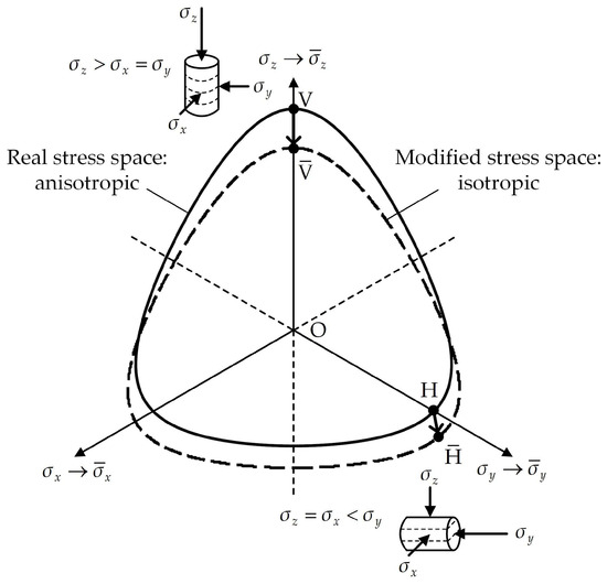
Figure 1. First step of mapping: from the real stress space to the modified stress space.

2.1.2. Formula

Now the work is to find a stress mapping formula satisfying Equation (1). Based on the works of Tobita and Yanagisawa [24] and Yao et al. [25], a new formula is proposed for the modified stress tensor:

$${\overline{\sigma }}_{ij}=\frac{3}{2}\left({\sigma }_{ik}{F}_{kj}+F_{ik}{\sigma }_{kj}\right)-s_{mn}{F}_{nm}{\delta }_{ij}$$

(2)

where $F_{ij}$ is the fabric tensor; $s_{ij}$ ($={\sigma }_{ij}-p{\delta }_{ij}$) is the deviatoric stress tensor; and ${\delta }_{ij}$ is the Kronecker delta. $F_{ij}$ is a well-known quantity that describes the microstructure of granular materials, and it can be defined by the spatial distribution of the particle long axis, contact normal, and void long axis. In this paper, a simple definition is adopted as follows:

$$F_{ij}=\frac{1}{N}{\displaystyle \sum _{k=1}^N{n}_i^k{n}_j^k}$$

(3)

where $N$ is the total number of soil particles in the specimen; superscript $k$ is the particle ID; and $\left(n_z,n_x,n_y\right)$ is the unit vector along the long axis of the $k$-th particle. It can be derived from Equation (3) that $F_{ij}$ is a symmetric second-order tensor, with its trace being equal to 1. The value of any given element in $F_{ij}$ represents the concentrated degree of particle long axes towards the corresponding direction. For the horizontally deposited soil, $F_{ij}$ can be expressed into

$$F_{ij}=\left(\begin{array}{ccc}\Delta & 0& 0\\ 0& \frac{1-\Delta }{2}& 0\\ 0& 0& \frac{1-\Delta }{2}\end{array}\right)$$

(4)

where $\Delta$ is a material parameter quantifying the anisotropic degree. Because the particle long axis tends to lie down on the horizontal plane, $\Delta$ is usually less than $1/3$. If $\Delta =1/3$, the soil is isotropic.

Based on Equations (2) and (4), ${\sigma }_z$ decreases after the stress modification, while ${\sigma }_x$ and ${\sigma }_y$ increases, because $\Delta <1/3$. Points $\mathrm{V}$ and $\mathrm{H}$ are mapped downwards to points $\overline{\mathrm{V}}$ and $\overline{\mathrm{H}}$, respectively, as shown in Figure 1. Therefore, the difference in yield strength along vertical and horizontal directions is narrowed, and the soil could be treated to be isotropic in the modified stress space. Compared with the formula in the works of Tobita and Yanagisawa [24] and Yao et al. [25], Equation (2) can ensure $\overline{p}=p$ for any ${\sigma }_{ij}$ and $F_{ij}$. It is necessary to note that keeping the mean stress unchanged is very important for the development of the soil constitutive model, because soil is a non-linear and pressure-dependent material. If the mean stress varies, the stiffness, strength, and many other properties of the soil are changed. We cannot distinguish whether the difference in the prediction results obtained using the constitutive model is caused by the variation of the loading direction or by that of the mean stress. What is more, there are some constitutive ingredients that are only related to $p$, but independent of the loading direction and soil fabric, such as the critical state stress ratio and void ratio (Li and Dafalias [26]; Wang et al. [27]; Deng et al. [28]). A varying $\overline{p}$ cannot guarantee the uniqueness of the critical state line. Equation (2) can avoid this problem without much revision to the modified stress method.

2.1.3. A Simple DEM Verification

A series of biaxial loading tests are conducted using discrete element method (DEM) software PFC2D 5.0 to preliminarily verify Equation (2). The size of the specimen is 35 mm × 35 mm and consists of more than 9000 elliptical particles. These particles are rigid aggregates of five circular particles, with the ratio of the long axis and short axis being 1.52, so that obvious anisotropy can be produced. The simplest model, i.e., the linear elastic perfectly plastic model, is adopted as the contact law. The model parameters are as follows: the normal contact stiffness between particles is 6.0 × 10⁸ N/m, the tangential stiffness is 4.0 × 10⁸ N/m, and the friction angle is 30°. The specimen is first generated under an isotropic pressure of 100 kPa, and then loaded in the case of a constant stress ratio, i.e., ${\sigma }_z$ and ${\sigma }_x$ increases proportionally while ${\sigma }_z/{\sigma }_x$ is kept unchanged. The reason why this kind of test is chosen is that the stress level is certain, and we just need to focus on the fabric evolution, which reduces the degree of freedom when a quantitative relation between ${\sigma }_{ij}$ and $F_{ij}$ is established.

Figure 2 shows the evolution of the second partial invariant of $F_{ij}$, i.e., $J_2=\left(F_{ij}-{\delta }_{ij}/2\right)\left(F_{ij}-{\delta }_{ij}/2\right)/2$, during the loading process. Because a 2D simulation is performed, the specimen is isotropic when $F_{ij}={\delta }_{ij}/2$ or $J_2=0$, which is the case at the beginning of the test. As ${\sigma }_z$ increases, the anisotropy degree is enhanced, since more and more particle long axes turn to be horizontal. Finally, when the external loading is large enough, $J_2$ converges to a limit value. That is to say, there is a state for the microstructure that can well adapt to the current stress level. The larger the stress ratio is, the heavier the fabric anisotropy is. The relation between ${\sigma }_z/{\sigma }_x$ and the limit value of $J_2$ is drawn in Figure 3, where the vertical coordinates are normalized by the limit value of $J_2$ when ${\sigma }_z/{\sigma }_x=1.1$. A parabolic curve can be observed when $F_{ij}$ is analyzed. However, if $F_{ij}$ and ${\sigma }_{ij}$ are combined through Equation (2), the modified stress ratio tensor ${\overline{\eta }}_{ij}$ ($={\overline{\sigma }}_{ij}/p$) has a normalized second partial invariant whose limit value is basically independent of ${\sigma }_z/{\sigma }_x$. Given that the second partial invariant corresponding to ${\sigma }_z/{\sigma }_x=1.1$ is very small, we can conclude that from the view of ${\overline{\sigma }}_{ij}$, the soil fabric can be approximately treated to be isotropic. It must be admitted that this conclusion is obtained under a very specific condition (we use oval-shaped particles, 2D simulation, and the constant stress ratio test, and the limit value must be reached), so that the above verification of Equation (2) is very preliminary. However, it provides a potential way to develop a multiscale constitutive model. Further verification is performed by comparisons with the experimental data in a later section.

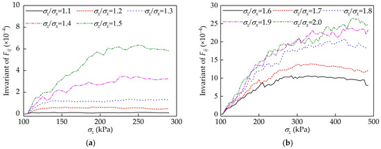
Figure 2. Evolution of the fabric tensor during the constant stress ratio tests: (a) σ_z/σ_x = 1.1~1.5; (b) σ_z/σ_x = 1.6~2.0.

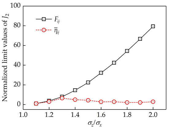
Figure 3. Relation between the stress ratio and the normalized limit value of J₂.

2.2. Transformed Stress Tensor

The first step of stress mapping simplifies the soil property to be isotropic, but it complicates the stress state because $F_{ij}$ is integrated into ${\overline{\sigma }}_{ij}$. Take the triaxial compression stress state, with ${\sigma }_y$ being the major principal stress, as an example. Due to the different fabric along the z- and x-axes, ${\overline{\sigma }}_z$ and ${\overline{\sigma }}_x$ are not equal, so the modified stress state is a true triaxial stress state (observe from Figure 1 that point $\overline{\mathrm{H}}$ is not located on the coordinate axis in the modified stress space). Such a complex ${\overline{\sigma }}_{ij}$ cannot be introduced directly into the existing constitutive models, which are established based on the triaxial compression behaviors of soil. Therefore, to develop an anisotropic model using ${\overline{\sigma }}_{ij}$, further steps must be taken to consider the effect of the intermediate principal stress.

2.2.1. Basic Idea

Another step of stress mapping is used to generalize the constitutive model from triaxial compression to true triaxial stress state (Yao and Wang [29]). As shown in Figure 4, the yield/failure surface in the modified stress space is non-circular according to the Matsuoka–Nakai criterion, demonstrating the effect of the intermediate principal stress. After the stress mapping, it turns into the circumcircle of the original surface on the same deviatoric plane. Thus, in the new stress space, namely, the space of transformed stress ${\tilde{\sigma }}_{ij}$, the yield strength and critical state stress ratio under any 3D stress state are identical to those under triaxial compression. The above goal of this mapping is formulated as

$$\left\{\begin{array}{l}\tilde{p}=\overline{p}\\ \tilde{\theta }=\overline{\theta }\\ \tilde{q}={\overline{q}}_{\mathrm{c}}\end{array}\right.$$

(5)

where $\theta$ is the Lode’s angle; $q$ is the deviatoric stress; signs ‘-’ and ‘~’ denote that the entity is related to the modified and transformed stress tensors, respectively; and ${\overline{q}}_{\mathrm{c}}$ is the deviatoric stress at the triaxial compression state point on the yield surface (see point $\overline{\mathrm{V}}$ in Figure 4). Using ${\tilde{\sigma }}_{ij}$, the existing constitutive models for the triaxial compression stress state are also available for the true triaxial stress state.

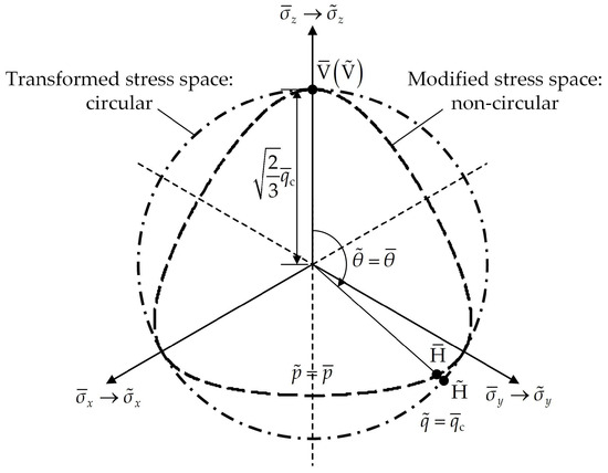
Figure 4. Second step of mapping: from the modified stress space to the transformed stress space.

2.2.2. Formula

According to the stress theory, the relation between the principal stresses and stress invariants is

$$\left\{\begin{array}{l}{\overline{\sigma }}_z=\overline{p}+\frac{2}{3}\overline{q}\cos \overline{\theta }\\ {\overline{\sigma }}_x=\overline{p}+\frac{2}{3}\overline{q}\cos \left(\overline{\theta }+\frac{2\pi }{3}\right)\\ {\overline{\sigma }}_y=\overline{p}+\frac{2}{3}\overline{q}\cos \left(\overline{\theta }-\frac{2\pi }{3}\right)\end{array}\right.$$

(6)

$$\left\{\begin{array}{l}{\tilde{\sigma }}_z=\tilde{p}+\frac{2}{3}\tilde{q}\cos \tilde{\theta }\\ {\tilde{\sigma }}_x=\tilde{p}+\frac{2}{3}\tilde{q}\cos \left(\tilde{\theta }+\frac{2\pi }{3}\right)\\ {\tilde{\sigma }}_y=\tilde{p}+\frac{2}{3}\tilde{q}\cos \left(\tilde{\theta }-\frac{2\pi }{3}\right)\end{array}\right.$$

(7)

By substituting Equation (5) into Equation (6) and comparing the results with Equation (7), we can obtain

$${\tilde{\sigma }}_i=\overline{p}+\frac{{\overline{q}}_{\mathrm{c}}}{\overline{q}}\left({\overline{\sigma }}_i-\overline{p}\right)$$

(8)

where $i=x,y,z$. Equation (8) provides a mapping between principal stress values, which can be directly extended to the tensor form

$${\tilde{\sigma }}_{ij}=\overline{p}{\delta }_{ij}+\frac{{\overline{q}}_{\mathrm{c}}}{\overline{q}}\left({\overline{\sigma }}_{ij}-\overline{p}{\delta }_{ij}\right)$$

(9)

According to Yao and Wang [29], ${\overline{q}}_{\mathrm{c}}$ can be derived from the Matsuoka–Nakai criterion as follows:

$${\overline{q}}_{\mathrm{c}}=\frac{{\overline{I}}_1{\overline{I}}_2-9{\overline{I}}_3+3\sqrt{\left({\overline{I}}_1{\overline{I}}_2-9{\overline{I}}_3\right)\left({\overline{I}}_1{\overline{I}}_2-{\overline{I}}_3\right)}}{4{\overline{I}}_2}$$

(10)

where ${\overline{I}}_1$, ${\overline{I}}_2$, and ${\overline{I}}_3$ are invariants of ${\overline{\sigma }}_{ij}$.

2.3. Brief Summary

The modified stress and transformed stress have some similarities. From the view of mathematics, both of them adjust the relative magnitude of different stress components using a mapping for the stress tensor, so that the problem is simplified in the new stress space. In terms of physical meaning, the modified stress establishes an equivalence between the isotropic and anisotropic soils, while the transformed stress establishes an equivalence between the soil behaviors under a triaxial compression stress state and those under a true triaxial stress state. These two steps can be used successively, so that the deformation and failure of anisotropic soils in a 3D stress space can be described. Note that the effect of soil anisotropy can also be reflected by modifying the material parameters in the isotropic model. For example, the internal friction angle, cohesion, modulus, and location of the critical state line can be assumed to be direction-dependent variables (Zhou et al. [30]; Gao and Zhao [31]; Yuan et al. [32]; Xie et al. [33]). Therefore, the calculated deformation and strength along different directions will certainly be different. The effect of the intermediate principal stress is usually considered by introducing a shape function, i.e., $g\left(\theta \right)$, into the 2D yield function. The critical state stress ratio becomes a function of the Lode’s angle (Tian and Zheng [34]; Du et al. [35]; Xue et al. [36]). By using different equations to modify the model parameters, this kind of method can provide an accurate prediction for the experimental results. However, this method makes the elastoplastic stiffness matrix very complex, because we have to compute the partial derivatives of these parameters with respect to the stress. On the other hand, the anisotropic constitutive model developed using the proposed method has a concise stiffness matrix (see Section 5.4), which brings much convenience for its numerical application.

3. Anisotropic Yield Surface

Because the inherent anisotropy is equivalent to isotropy, the existing isotropic constitutive model is available for anisotropic soils by replacing ${\sigma }_{ij}$ with ${\tilde{\sigma }}_{ij}$ directly. For example, based on the modified Cam-clay (MCC) model, the anisotropic yield function can be written as

$$f={\tilde{q}}^2+{\tilde{M}}^2\tilde{p}\left(\tilde{p}-{\tilde{p}}_x\right)=0$$

(11)

where $\tilde{M}$ is the critical state stress ratio in the transformed stress space, and its relation to the original critical state stress ratio $M$ is shown later; ${\tilde{p}}_x$ controls the size of the yield surface. By substituting Equations (2) and (9) into Equation (11), we can obtain an anisotropic yield surface in the real stress space. Characteristics of this yield surface is analyzed in the next section.

3.1. In 3D Stress Space

The anisotropic yield surface in a 3D stress space is shown in Figure 5. It can be seen that the yield surface rotates towards the ${\sigma }_z$-axis, indicating a greater yield strength along this direction. The hydrostatic axis where ${\sigma }_z={\sigma }_x={\sigma }_y$ does not pass through the vertex of the yield surface. The yield surface is not an ellipsoid, because it has different intercepts for different Lode’s angles, especially when $p$ is relatively smaller. Wheeler et al. [6] pointed out that if the $g\left(\theta \right)$ method is adopted to generalize the rotated yield surface to a 3D stress space, a singularity appears. Based on the proposed method, the 3D anisotropic yield surface is continuous and smooth, showing its good performance in describing the yield property of the anisotropic soil in a complex stress state. Moreover, the proposed method is also capable of generalizing other kinds of yield surfaces or bounding surfaces, other than the elliptical yield surface of the MCC model.

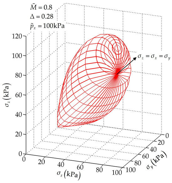
Figure 5. Yield surface of the anisotropic MCC model in 3D stress space.

3.2. On the Triaxial Meridian Plane

To illustrate the anisotropic yield surface more clearly, its section on the triaxial meridian plane ($\theta =0°~180°$) is drawn in Figure 6. The vertical coordinate is ${\sigma }_z-{\sigma }_x$, rather than $q$, because $q$ is non-negative. The upper part of this figure denotes the triaxial compression stress state (${\sigma }_z>{\sigma }_x={\sigma }_y$), while the lower part is the triaxial extension (${\sigma }_z<{\sigma }_x={\sigma }_y$). Observe that the 2D yield surface rotates upwards to an axis with a slope of $3\left(1-3\Delta \right)/\left(1+3\Delta \right)$. For a heavier degree of fabric anisotropy, i.e., a smaller $\Delta$, the rotation angle becomes larger. At the intersection of the yield surface with the $p$-axis, the outer normal vector is marked in Figure 6. This vector points downwards, which means the vertical plastic strain increment $\mathrm{d}{\epsilon }_z^{\mathrm{p}}$ is smaller than the horizontal plastic strain increment $\mathrm{d}{\epsilon }_x^{\mathrm{p}}$ if an associated flow rule is adopted. This characteristic conforms to the results of the isotropic compression tests on anisotropic sand (Lade and Abelev [37]). Figure 6 also shows the anisotropic yield surface obtained by Wheeler et al. [6] (see the broken line), which is obtained by rotating the isotropic yield surface (the yield function is listed in Table 1). Compared with it, the anisotropic yield surface shown in this paper is much flatter, especially on the triaxial extension side. This is because the effect of the intermediate principal stress is taken into consideration by the transformed stress.

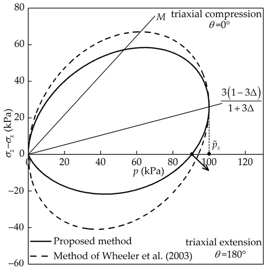
Figure 6. Yield surface of the anisotropic MCC model on the triaxial meridian plane [6].

In fact, the anisotropic MCC model developed using the proposed method adopts a virtual plastic work increment as follows:

$$\mathrm{d}{\tilde{W}}^{\mathrm{p}}=\tilde{p}\cdot \mathrm{d}{\epsilon }_{\mathrm{v}}^{\mathrm{p}}+\tilde{q}\cdot \mathrm{d}{\epsilon }_{\mathrm{d}}^{\mathrm{p}}=\tilde{p}\sqrt{{\left(\mathrm{d}{\epsilon }_{\mathrm{v}}^{\mathrm{p}}\right)}^2+{\left(\tilde{M}\cdot \mathrm{d}{\epsilon }_{\mathrm{d}}^{\mathrm{p}}\right)}^2}$$

(12)

where $\mathrm{d}{\epsilon }_{\mathrm{v}}^{\mathrm{p}}$ is the plastic volumetric strain increment, and $\mathrm{d}{\epsilon }_{\mathrm{d}}^{\mathrm{p}}$ is the plastic deviatoric strain increment. This plastic work increment has a similar form to that of the isotropic MCC model, except for the substitution of stress. The anisotropic yield function (i.e., Equation (11)) can be derived from Equation (12) using an associated flow rule. For the stress state at point $\mathrm{V}$ in Figure 1, by substituting Equations (2) and (9) into Equation (12), we can determine the real plastic work increment as follows:

$$\mathrm{d}{W}^{\mathrm{p}}=p\cdot \mathrm{d}{\epsilon }_{\mathrm{v}}^{\mathrm{p}}+q\cdot \mathrm{d}{\epsilon }_{\mathrm{d}}^{\mathrm{p}}=p\sqrt{{\left(\mathrm{d}{\epsilon }_{\mathrm{v}}^{\mathrm{p}}\right)}^2+{\left(\tilde{M}\cdot \mathrm{d}{\epsilon }_{\mathrm{d}}^{\mathrm{p}}\right)}^2+{\alpha }^{\prime }\cdot \mathrm{d}{\epsilon }_{\mathrm{v}}^{\mathrm{p}}\cdot \mathrm{d}{\epsilon }_{\mathrm{d}}^{\mathrm{p}}}$$

(13)

where

$${\alpha }^{\prime }=\frac{1-3\Delta }{1+3\Delta }\cdot \frac{2\left(\tilde{\eta }+3\right)}{{\tilde{M}}^2-{\tilde{\eta }}^2}\left[{\tilde{M}}^2+\frac{2{\tilde{\eta }}^2+3\left(1-3\Delta \right)\tilde{\eta }}{1+3\Delta }\right]$$

(14)

where $\tilde{\eta }=\tilde{q}/\tilde{p}$. ${\alpha }^{\prime }$ is just the back stress that works as an anisotropic variable to rotate the yield surface in the references. When the soil is isotropic ($\Delta =1/3$), ${\alpha }^{\prime }=0$, so that the anisotropic yield function degrades into the isotropic yield function. Therefore, Equation (14) provides a microscopic interpretation for the back stress in thermodynamics.

3.3. On the Deviatoric Plane

Figure 7 integrates the cross sections of the 3D anisotropic yield surface on different deviatoric planes. When $p=99 \mathrm{kPa}$, the yield surface is very small and close to a circle whose center is located on the positive axis of ${\sigma }_z$. As $p$ decreases (i.e., the stress ratio $q/p$ increases), the yield surface becomes bigger, and its shape tends to be triangular. The intercept of the yield surface on the ${\sigma }_z$-axis is larger than that on the ${\sigma }_x$- and ${\sigma }_y$-axes, while the triaxial extension stress state with ${\sigma }_z<{\sigma }_x={\sigma }_y$ has the lowest yield strength. Therefore, the proposed method can reflect the complex coupling effect of the inherent anisotropy and intermediate principal stress.

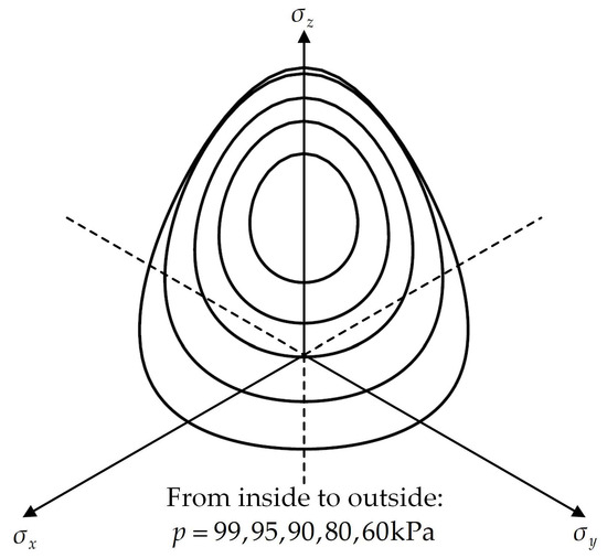
Figure 7. Yield surface of the anisotropic MCC model on the deviatoric plane.

4. Induced Anisotropy

During the loading process, the applied stress causes a redistribution of soil particles, and hence, changes the anisotropic degree of stiffness and strength along different directions. This induced anisotropy is often described by a rotational hardening law in the references (see Table 1). Because the rotation angle of the anisotropic yield surface in this paper is controlled by the fabric tensor, a fabric evolution law can play the same role as the rotational hardening law in the constitutive model (Zhao and Kruyt [38]). According to many DEM simulations (Wen and Zhang [39]; Wang et al. [40]; Sufian et al. [41]), particle long axes are reoriented towards the principal stress direction, although their rotation is much slower than that of contact normals. At the critical state, the preferred particle orientation is perpendicular to the major principal stress, while the anisotropic degree reaches a stable value that is only determined by the stress state. Similar results can also be observed from the constant stress ratio tests in Section 2.1.3. Based on these microscopic statistics and by imitating the form of the rotational hardening law, we hereby propose the following fabric evolution law:

$$\mathrm{d}{F}_{ij}=C\frac{1+e_0}{\lambda -\kappa }\frac{\mathrm{d}{\epsilon }_{\mathrm{v}}^{\mathrm{p}}}{\tilde{M}-\tilde{\eta }}\left(\frac{{\delta }_{ij}}{3}-\beta {\eta }_{ij}-F_{ij}\right)$$

(15)

where $C$ is a new parameter controlling the fabric evolution rate; $e_0$ is the initial void ratio; $\lambda$ and $\kappa$ are the compression and swelling indexes of the MCC model, respectively; and $\beta$ is another parameter defining the final state of the fabric evolution. The increment of $F_{ij}$ is assumed to be proportional to that of ${\epsilon }_{\mathrm{v}}^{\mathrm{p}}$, just like the equations of $\mathrm{d}\alpha$ in the works of Wheeler et al. [6] and Seidalinov and Taiebat [14]. The term $\tilde{M}-\tilde{\eta }$ is introduced to slow down the fabric evolution rate at the beginning of the loading process. According to the dilatancy function of the anisotropic MCC model (which can be easily derived from Equation (12)), $\mathrm{d}{\epsilon }_{\mathrm{v}}^{\mathrm{p}}/\left(\tilde{M}-\tilde{\eta }\right)$ is equal to a function of $\mathrm{d}{\epsilon }_{\mathrm{d}}^{\mathrm{p}}$, which is not zero at the critical state. Therefore, the introduction of $\tilde{M}-\tilde{\eta }$ makes the anisotropy stop evolving only when $F_{ij}$ reaches its own critical state value. In the last term, ${\delta }_{ij}/3-\beta {\eta }_{ij}$ works as an ‘attractor’ for $F_{ij}$, in the sense that the principal axes of $F_{ij}$ are forced to rotate towards the principal stress axes, while the value of $F_{ij}$ converges to ${\delta }_{ij}/3-\beta {\eta }_{ij}$ at the critical state. Substituting $F_{ij}={\delta }_{ij}/3-\beta {\eta }_{ij}$ into Equations (2) and (9) gives the relation between $\tilde{M}$ and $M$:

$$\tilde{M}=M-\beta M\left(M+3\right)$$

(16)

The fabric evolution law in Equation (15) links the microscopic particle arrangement (denoted by $\mathrm{d}{F}_{ij}$) to the macroscopic soil deformation (denoted by $\mathrm{d}{\epsilon }_{\mathrm{v}}^{\mathrm{p}}$). Compared with the rotational hardening law, the proposed fabric evolution law can grasp the discrete feature of soil as a granular material.

5. Anisotropic MCC Model

Using ${\tilde{\sigma }}_{ij}$, the existing 2D isotropic constitutive model can be generalized into a 3D anisotropic model. In this paper, the MCC model is adopted as an example for the generalization. Its yield function is established and analyzed in Section 3. What follows introduces the plastic flow rule and hardening law of the anisotropic MCC model, and derives the elastoplastic stiffness matrix for the numerical application.

5.1. Plastic Flow Rule

Similar to the anisotropic yield function (Equation (11)), the plastic flow rule can be directly generalized to be anisotropic by replacing ${\sigma }_{ij}$ with ${\tilde{\sigma }}_{ij}$

$$\mathrm{d}{\epsilon }_{ij}^{\mathrm{p}}=\Lambda \frac{\partial f}{\partial {\tilde{\sigma }}_{ij}}$$

(17)

where $\Lambda$ is the plastic multiplier that can be derived from the consistency condition $\mathrm{d}f=0$. It is necessary to emphasize that the plastic flow direction is assumed to be normal to the yield surface in the transformed stress space, rather than the yield surface in the real stress space. This is because the intersection of the rotated yield surface with the critical state line is not the peak point (see Figure 6), which leads to a non-zero $\mathrm{d}{\epsilon }_{\mathrm{v}}^{\mathrm{p}}$ at the critical state if normality holds in the real stress space. Therefore, strictly speaking, the plastic flow rule is non-associated.

5.2. Hardening Law

The hardening law of the anisotropic MCC model can be expressed as follows:

$$\mathrm{d}{\tilde{p}}_x=\frac{1+e_0}{\lambda -\kappa }{\tilde{p}}_x\mathrm{d}{\epsilon }_{\mathrm{v}}^{\mathrm{p}}$$

(18)

This equation determines the size change of the yield surface during the strain hardening process, while Equation (15) makes the yield surface rotate until the critical state of the fabric tensor is reached.

5.3. Elastic Stiffness Matrix

For simplicity, the elasticity anisotropy is ignored so that the elastic stress–strain relation is calculated by the isotropic Hooke’s law:

$$\mathrm{d}{\sigma }_{ij}=D_{ijkl}^{\mathrm{e}}\mathrm{d}{\epsilon }_{kl}^{\mathrm{e}}=D_{ijkl}^{\mathrm{e}}\left(\mathrm{d}{\epsilon }_{kl}-\mathrm{d}{\epsilon }_{kl}^{\mathrm{p}}\right)$$

(19)

where $\mathrm{d}{\epsilon }_{kl}$ is the total strain increment tensor; $\mathrm{d}{\epsilon }_{kl}^{\mathrm{e}}$ is the elastic strain increment tensor; and $D_{ijkl}^{\mathrm{e}}$ is the elastic stiffness matrix as follows:

$$D_{ijkl}^{\mathrm{e}}=\left(K-\frac{2}{3}G\right){\delta }_{ij}{\delta }_{kl}+G\left({\delta }_{ik}{\delta }_{jl}+{\delta }_{il}{\delta }_{jk}\right)$$

(20)

where the bulk modulus $K$ and shear modulus $G$ are pressure dependent:

$$K=\frac{1+e_0}{\kappa }p$$

(21)

$$G=\frac{3\left(1-2\nu \right)\left(1+e_0\right)}{2\left(1+\nu \right)\kappa }p$$

(22)

where $\nu$ is Poisson’s ratio.

5.4. Elastoplastic Stiffness Matrix

If the elastic trial stress state point comes out of the yield surface, the stress–strain relation should be recalculated using the elastoplastic stiffness matrix. According to the consistency condition,

$$\mathrm{d}f=\frac{\partial f}{\partial {\sigma }_{ij}}\mathrm{d}{\sigma }_{ij}+\frac{\partial f}{\partial F_{st}}\mathrm{d}{F}_{st}+\frac{\partial f}{\partial {\tilde{p}}_x}\mathrm{d}{\tilde{p}}_x=0$$

(23)

Note that $\partial f/\partial {\sigma }_{ij}$, rather than $\partial f/\partial {\tilde{\sigma }}_{ij}$ or $\partial f/\partial {\overline{\sigma }}_{ij}$, should be introduced because we have to determine the relation between $\mathrm{d}{\sigma }_{ij}$ and $\mathrm{d}{\epsilon }_{kl}$. By substituting the fabric evolution law (Equation (15)), the hardening law (Equation (18)), and the elastic stress–strain relation (Equation (19)) into Equation (23), we can obtain

$$\frac{\partial f}{\partial {\sigma }_{ij}}{D}_{ijkl}^{\mathrm{e}}\left(\mathrm{d}{\epsilon }_{kl}-\mathrm{d}{\epsilon }_{kl}^{\mathrm{p}}\right)+\frac{\partial f}{\partial F_{st}}\frac{\partial F_{st}}{\partial {\epsilon }_{\mathrm{v}}^{\mathrm{p}}}\mathrm{d}{\epsilon }_{\mathrm{v}}^{\mathrm{p}}+\frac{\partial f}{\partial {\tilde{p}}_x}\frac{\partial {\tilde{p}}_x}{\partial {\epsilon }_{\mathrm{v}}^{\mathrm{p}}}\mathrm{d}{\epsilon }_{\mathrm{v}}^{\mathrm{p}}=0$$

(24)

Then, $\Lambda$ is worked out by combining Equations (17) and (24):

$$\Lambda =\frac{\frac{\partial f}{\partial {\sigma }_{ij}}{D}_{ijkl}^{\mathrm{e}}\mathrm{d}{\epsilon }_{kl}}{\frac{\partial f}{\partial {\sigma }_{ij}}{D}_{ijkl}^{\mathrm{e}}\frac{\partial f}{\partial {\tilde{\sigma }}_{kl}}-\left(\frac{\partial f}{\partial F_{st}}\frac{\partial F_{st}}{\partial {\epsilon }_{\mathrm{v}}^{\mathrm{p}}}+\frac{\partial f}{\partial {\tilde{p}}_x}\frac{\partial {\tilde{p}}_x}{\partial {\epsilon }_{\mathrm{v}}^{\mathrm{p}}}\right)\frac{\partial f}{\partial \tilde{p}}}$$

(25)

Finally, if Equations (17) and (25) are substituted back into Equation (19), the elastoplastic stiffness matrix can be determined as follows:

$$D_{ijkl}^{\mathrm{ep}}=D_{ijkl}^{\mathrm{e}}-\frac{D_{ijmn}^{\mathrm{e}}\frac{\partial f}{\partial {\tilde{\sigma }}_{mn}}\frac{\partial f}{\partial {\sigma }_{pq}}{D}_{pqkl}^{\mathrm{e}}}{\frac{\partial f}{\partial {\sigma }_{pq}}{D}_{pqmn}^{\mathrm{e}}\frac{\partial f}{\partial {\tilde{\sigma }}_{mn}}-\left(\frac{\partial f}{\partial F_{st}}\frac{\partial F_{st}}{\partial {\epsilon }_{\mathrm{v}}^{\mathrm{p}}}+\frac{\partial f}{\partial {\tilde{p}}_x}\frac{\partial {\tilde{p}}_x}{\partial {\epsilon }_{\mathrm{v}}^{\mathrm{p}}}\right)\frac{\partial f}{\partial \tilde{p}}}$$

(26)

where some repeated subscripts are replaced to avoid misunderstanding. In Equation (26), partial derivatives $\frac{\partial f}{\partial {\tilde{\sigma }}_{mn}}$, $\frac{\partial f}{\partial {\tilde{p}}_x}$, and $\frac{\partial {\tilde{p}}_x}{\partial {\epsilon }_{\mathrm{v}}^{\mathrm{p}}}$ can be easily obtained from the anisotropic yield function (i.e., Equation (11)) and hardening law (i.e., Equation (18)). Compared with the corresponding partial derivatives of the isotropic MCC model, they have similar forms, except that ${\sigma }_{ij}$ is replaced by ${\tilde{\sigma }}_{ij}$. Moreover, based on the chain rule, partial derivatives $\frac{\partial f}{\partial {\sigma }_{pq}}$ and $\frac{\partial f}{\partial F_{st}}$ are calculated as follows:

$$\frac{\partial f}{\partial {\sigma }_{pq}}=\frac{\partial f}{\partial {\overline{\sigma }}_{ij}}\frac{\partial {\overline{\sigma }}_{ij}}{\partial {\sigma }_{pq}}=\left(\frac{\partial f}{\partial \tilde{p}}\frac{\partial \tilde{p}}{\partial {\overline{\sigma }}_{ij}}+\frac{\partial f}{\partial \tilde{q}}\frac{\partial \tilde{q}}{\partial {\overline{\sigma }}_{ij}}\right)\left[\frac{3}{2}\left({\delta }_{ip}{F}_{qj}+F_{ip}{\delta }_{qj}\right)-\left(F_{qp}-\frac{1}{3}{\delta }_{qp}\right){\delta }_{ij}\right]$$

(27)

$$\frac{\partial f}{\partial F_{st}}=\frac{\partial f}{\partial {\overline{\sigma }}_{ij}}\frac{\partial {\overline{\sigma }}_{ij}}{\partial F_{st}}=\left(\frac{\partial f}{\partial \tilde{p}}\frac{\partial \tilde{p}}{\partial {\overline{\sigma }}_{ij}}+\frac{\partial f}{\partial \tilde{q}}\frac{\partial \tilde{q}}{\partial {\overline{\sigma }}_{ij}}\right)\left[\frac{3}{2}\left({\sigma }_{is}{\delta }_{tj}+{\delta }_{is}{\sigma }_{tj}\right)-s_{ts}{\delta }_{ij}\right]$$

(28)

According to Equation (5), partial derivatives $\frac{\partial \tilde{p}}{\partial {\overline{\sigma }}_{ij}}$ and $\frac{\partial \tilde{q}}{\partial {\overline{\sigma }}_{ij}}$ in the above equations are equal to

$$\frac{\partial \tilde{p}}{\partial {\overline{\sigma }}_{ij}}=\frac{\partial \overline{p}}{\partial {\overline{\sigma }}_{ij}}=\frac{1}{3}{\delta }_{ij}$$

(29)

$$\frac{\partial \tilde{q}}{\partial {\overline{\sigma }}_{ij}}=\frac{\partial {\overline{q}}_{\mathrm{c}}}{\partial {\overline{\sigma }}_{ij}}=\frac{\partial {\overline{q}}_{\mathrm{c}}}{\partial {\overline{I}}_1}\frac{\partial {\overline{I}}_1}{\partial {\overline{\sigma }}_{ij}}+\frac{\partial {\overline{q}}_{\mathrm{c}}}{\partial {\overline{I}}_2}\frac{\partial {\overline{I}}_2}{\partial {\overline{\sigma }}_{ij}}+\frac{\partial {\overline{q}}_{\mathrm{c}}}{\partial {\overline{I}}_3}\frac{\partial {\overline{I}}_3}{\partial {\overline{\sigma }}_{ij}}$$

(30)

It can be seen from Equation (26) that the elastoplastic stiffness matrix of the anisotropic MCC model is in a similar form as its general formula, which should be attributed to the proposed method to consider the effect of the inherent and induced anisotropy. When the anisotropic MCC model is applied to calculating the stress–strain relation, $D_{ijkl}^{\mathrm{e}}$ or $D_{ijkl}^{\mathrm{ep}}$ can be first determined by the values of ${\sigma }_{ij}$ and $F_{ij}$ at the beginning of the incremental step, according to Equation (20) or Equation (26). Then, by substituting the boundary conditions into the stress–strain relation functions, we can work out $\mathrm{d}{\sigma }_{ij}$ and $\mathrm{d}{\epsilon }_{ij}$ for this incremental step. The variation of the soil fabric, i.e., $\mathrm{d}{F}_{ij}$, can also be obtained by Equation (15). As a result, the values of ${\sigma }_{ij}$, ${\epsilon }_{ij}$, and $F_{ij}$ are updated for the calculation of the next incremental step. Note that ${\overline{\sigma }}_{ij}$ and ${\tilde{\sigma }}_{ij}$ just provide a mathematical tool for considering the effects of the soil anisotropy and intermediate principal stress. The obtained stress–strain relation still refers to the relation between $\mathrm{d}{\sigma }_{ij}$ and $\mathrm{d}{\epsilon }_{ij}$, rather than $\mathrm{d}{\overline{\sigma }}_{ij}$ or $\mathrm{d}{\tilde{\sigma }}_{ij}$ and $\mathrm{d}{\epsilon }_{ij}$.

5.5. Comparison between the Isotropic and Anisotropic MCC Models

Table 2 summarizes the governing equations of the isotropic and anisotropic MCC models. We can find that, compared with the isotropic model, the anisotropic MCC model just replaces ${\sigma }_{ij}$ with ${\tilde{\sigma }}_{ij}$ and preserves the original form of the model framework. This method is also capable of developing other isotropic models. According to the summary in the introduction, if the governing equations of the isotropic model are expressed as $f\left({\sigma }_{ij}\right)=0$, an anisotropic model can be directly developed as $f\left({\tilde{\sigma }}_{ij}\right)=0$.

Table 2. Governing equations of the isotropic and anisotropic MCC models.

	Isotropic MCC Model	Anisotropic MCC Model
Stress tensor	${\sigma }_{ij}$	${\tilde{\sigma }}_{ij}=\overline{p}{\delta }_{ij}+\frac{{\overline{q}}_{\mathrm{c}}}{\overline{q}}\left({\overline{\sigma }}_{ij}-\overline{p}{\delta }_{ij}\right)$ $\mathrm{where} {\overline{\sigma }}_{ij}=\frac{3}{2}\left({\sigma }_{ik}{F}_{kj}+F_{ik}{\sigma }_{kj}\right)-s_{mn}{F}_{nm}{\delta }_{ij}$
Yield function	$f=q^2+M^{2}p\left(p-p_x\right)=0$	$f={\tilde{q}}^2+{\tilde{M}}^2\tilde{p}\left(\tilde{p}-{\tilde{p}}_x\right)=0$
Plastic flow rule	$\mathrm{d}{\epsilon }_{ij}^{\mathrm{p}}=\Lambda \frac{\partial f}{\partial {\sigma }_{ij}}$	$\mathrm{d}{\epsilon }_{ij}^{\mathrm{p}}=\Lambda \frac{\partial f}{\partial {\tilde{\sigma }}_{ij}}$
Hardening law	$\mathrm{d}{p}_x=\frac{1+e_0}{\lambda -\kappa }{p}_x\mathrm{d}{\epsilon }_{\mathrm{v}}^{\mathrm{p}}$	$\mathrm{d}{\tilde{p}}_x=\frac{1+e_0}{\lambda -\kappa }{\tilde{p}}_x\mathrm{d}{\epsilon }_{\mathrm{v}}^{\mathrm{p}}$ $\mathrm{and} \mathrm{d}{F}_{ij}=C\frac{1+e_0}{\lambda -\kappa }\frac{\mathrm{d}{\epsilon }_{\mathrm{v}}^{\mathrm{p}}}{\tilde{M}-\tilde{\eta }}\left(\frac{{\delta }_{ij}}{3}-\beta {\eta }_{ij}-F_{ij}\right)$
Elastic stiffness matrix	$D_{ijkl}^{\mathrm{e}}=\left(K-\frac{2}{3}G\right){\delta }_{ij}{\delta }_{kl}+G\left({\delta }_{ik}{\delta }_{jl}+{\delta }_{il}{\delta }_{jk}\right)$$, \mathrm{where} K=\frac{1+e_0}{\kappa }p$$\mathrm{and} G=\frac{3\left(1-2\nu \right)\left(1+e_0\right)}{2\left(1+\nu \right)\kappa }p$
Elastoplastic stiffness matrix	$D_{ijkl}^{\mathrm{ep}}=D_{ijkl}^{\mathrm{e}}-\frac{D_{ijmn}^{\mathrm{e}}\frac{\partial f}{\partial {\sigma }_{mn}}\frac{\partial f}{\partial {\sigma }_{pq}}{D}_{pqkl}^{\mathrm{e}}}{\frac{\partial f}{\partial {\sigma }_{pq}}{D}_{pqmn}^{\mathrm{e}}\frac{\partial f}{\partial {\sigma }_{mn}}-\frac{\partial f}{\partial p_x}\frac{\partial p_x}{\partial {\epsilon }_{\mathrm{v}}^{\mathrm{p}}}\frac{\partial f}{\partial p}}$	$D_{ijkl}^{\mathrm{ep}}=D_{ijkl}^{\mathrm{e}}-\frac{D_{ijmn}^{\mathrm{e}}\frac{\partial f}{\partial {\tilde{\sigma }}_{mn}}\frac{\partial f}{\partial {\sigma }_{pq}}{D}_{pqkl}^{\mathrm{e}}}{\frac{\partial f}{\partial {\sigma }_{pq}}{D}_{pqmn}^{\mathrm{e}}\frac{\partial f}{\partial {\tilde{\sigma }}_{mn}}-\left(\frac{\partial f}{\partial F_{st}}\frac{\partial F_{st}}{\partial {\epsilon }_{\mathrm{v}}^{\mathrm{p}}}+\frac{\partial f}{\partial {\tilde{p}}_x}\frac{\partial {\tilde{p}}_x}{\partial {\epsilon }_{\mathrm{v}}^{\mathrm{p}}}\right)\frac{\partial f}{\partial \tilde{p}}}$
Parameters	M, λ, κ, and ν	M, λ, κ, ν, Δ, C, and β

6. Verification of the Proposed Method

There are seven parameters in the anisotropic MCC model: M, λ, κ, ν, Δ, C, and β. The first four parameters are inherited from the isotropic MCC model and can be calibrated using the same method as before. The last three parameters reflect the initial value, evolution rate, and final value of the fabric tensor, respectively. Theoretically, they should be determined through microscopic statistics about the particle arrangement. In practice, their values can also be calibrated according to the soil stiffness along different directions. For example, during the isotropic compression test (which is used to determine λ and κ), strain increments perpendicular and parallel to the bedding plane, i.e., $\mathrm{d}{\epsilon }_z$ and $\mathrm{d}{\epsilon }_x$, can be measured during the loading process. The initial value of $\mathrm{d}{\epsilon }_z/\mathrm{d}{\epsilon }_x$ is dependent on the initial degree of the fabric anisotropy, while its variation is related to the fabric evolution. Based on this, the values of Δ and C can be determined by fitting the measured curve of $\mathrm{d}{\epsilon }_z/\mathrm{d}{\epsilon }_x$. Similarly, we can determine β using the stable value of $\mathrm{d}{\epsilon }_z/\mathrm{d}{\epsilon }_x$ during a constant stress ratio test.

The anisotropic MCC model is used to predict the stress ratio ${\sigma }_1/{\sigma }_3$ and pore pressure $u$ (normalized by the consolidation pressure ${\sigma }_{\mathrm{c}}$) of the horizontally deposited San Francisco Bay mud from true triaxial tests (Kirkgard and Lade [42]). This soil is normally consolidated. Under the same intermediate principal stress coefficient $b$, the Lode’s angle $\theta$ can be different when the principal stresses are along different directions: if $0°\le \theta <60°$, ${\sigma }_z$ is the major principal stress; if $60°<\theta <120°$, ${\sigma }_z$ is the intermediate principal stress; and if $120°<\theta <240°$, ${\sigma }_z$ is the minor principal stress. The model parameters are $M=1.54$, $\lambda =0.80$, $\kappa =0.13$, $\nu =0.30$, $\Delta =0.31$, $C=0.60$, and $\beta =0.025$. Comparisons between the experimental data and model predictions are shown in Figure 8. It can be concluded that the proposed method can reasonably simulate soil behaviors under different loading directions and intermediate principal stress coefficients. What is more, if the vertical strain ${\epsilon }_z$ continues increasing, ${\sigma }_1/{\sigma }_3$ and $u$ (as well as $F_{ij}$) finally converge to a stable value independent of the loading direction, which means the proposed method can guarantee the uniqueness of the critical state line. When $b=0.96$, the model predictions slightly deviate from the experimental data and cannot reproduce the decrease in ${\sigma }_1/{\sigma }_3$ with ${\epsilon }_z$. This is probably due to the strain localization of the soil specimen under the condition of extension, which cannot be simulated using the MCC model.

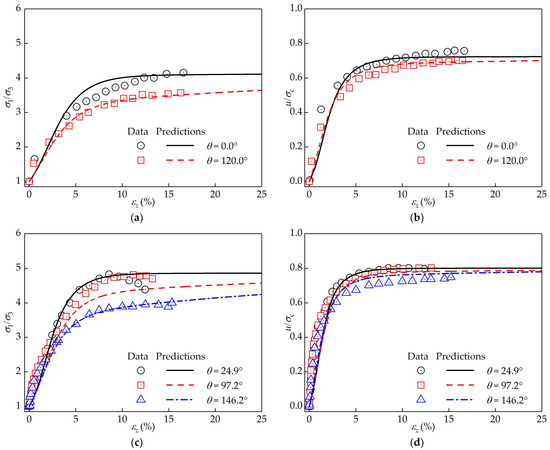
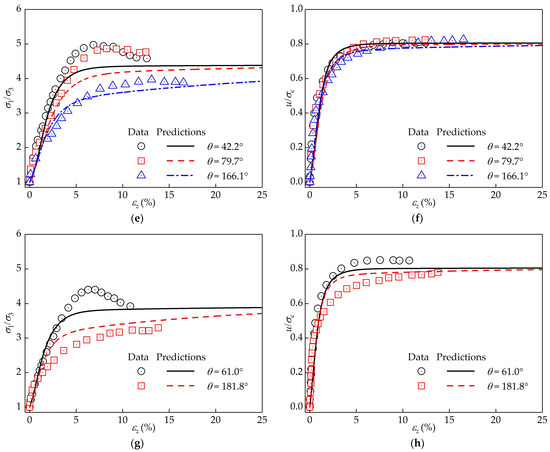
Figure 8. Comparisons between the experimental data and model predictions of the horizontally deposited San Francisco Bay mud from true triaxial tests: (a,b) b = 0.00; (c,d) b ≈ 0.42; (e,f) b ≈ 0.71; and (g,h) b ≈ 0.96.

7. Conclusions

In this paper, a multiscale method is proposed to develop an anisotropic constitutive model for soils by introducing the fabric tensor and its evolution. This method has the following characteristics:

• The inherent anisotropy is considered using two steps of stress mapping. From ${\sigma }_{ij}$ to ${\overline{\sigma }}_{ij}$, anisotropic soil is equivalent to isotropic soil; from ${\overline{\sigma }}_{ij}$ to ${\tilde{\sigma }}_{ij}$, the true triaxial yield/failure behaviors are similar to those of triaxial compression.
• The induced anisotropy is represented by a fabric evolution law, which plays the same role as the rotational hardening law but can capture the microscopic mechanism behind soil deformation.
• Based on an isotropic constitutive model, $f\left({\sigma }_{ij}\right)=0$, the anisotropic model $f\left({\tilde{\sigma }}_{ij}\right)=0$ can be easily developed to predict the stress–strain relation of anisotropic soil in a three-dimensional stress state.

It is necessary to indicate that the modified stress equation, i.e., Equation (2), is proposed according to the observed deformation and failure properties of anisotropic soils, and its verification in Section 2.1.3 is very preliminary. The fabric evolution law, i.e., Equation (15), is established by imitating the form of the rotational hardening law. We need to do further research, such as DEM simulations under complex loading conditions, to find a more precise expression for ${\overline{\sigma }}_{ij}$ that can realize the equivalence between the anisotropic and isotropic soils. A bridge should be built to truly connect the macroscopic and microscopic mechanical behaviors of soils.

References

- Lai, V.Q.; Shiau, J.; Keawsawasvong, S.; Seehavong, S.; Cabangon, L.T. Undrained stability of unsupported rectangular excavations: Anisotropy and non-homogeneity in 3D. Buildings 2022, 12, 1425. [Google Scholar] [CrossRef]
- Ng, C.W.W.; Qu, C.X.; Ni, J.J.; Guo, H.W. Three-dimensional reliability analysis of unsaturated soil slope considering permeability rotated anisotropy random fields. Comput. Geotech. 2022, 151, 104944. [Google Scholar] [CrossRef]
- Fang, Y.; Cui, J.; Wanatowski, D.; Nikitas, N.; Yuan, R.; He, Y. Subsurface settlements of shield tunneling predicted by 2D and 3D constitutive models considering non-coaxiality and soil anisotropy: A case study. Can. Geotech. J. 2022, 59, 424–440. [Google Scholar] [CrossRef]
- Sekiguchi, H.; Ohta, H. Induced anisotropy and time dependency in clays. In Proceedings of the 9th International Conference on Soil Mechanics and Foundation Engineering, Tokyo, Japan, 10–15 July 1977; pp. 229–238. [Google Scholar]
- Pestana, J.M.; Whittle, A.J. Formulation of a unified constitutive model for clays and sands. Int. J. Numer. Anal. Methods Geomech. 1999, 23, 1215–1243. [Google Scholar] [CrossRef]
- Wheeler, S.J.; Näätänen, A.; Karstunen, M.; Lojander, M. An anisotropic elastoplastic model for soft clays. Can. Geotech. J. 2003, 40, 403–418. [Google Scholar] [CrossRef]
- Niu, Y.Q.; Chang, D.; Wang, X.; Liao, M.K. Anisotropic constitutive model of frozen silty clay capturing ice cementation degradation under high mean stresses. J. Mater. Res. Technol.-JMRT 2023, 27, 1461–1472. [Google Scholar] [CrossRef]
- Shi, Z.H.; Hambleton, J.P.; Buscarnera, G. Bounding surface elasto-viscoplasticity: A general constitutive framework for rate-dependent geomaterials. J. Eng. Mech. 2019, 145, 04019002. [Google Scholar] [CrossRef]
- Zhao, Y.H.; Lai, Y.M.; Pei, W.S.; Yu, F. An anisotropic bounding surface elastoplastic constitutive model for frozen sulfate saline silty clay under cyclic loading. Int. J. Plast. 2020, 129, 102668. [Google Scholar] [CrossRef]
- Zhang, A.; Dafalias, Y.F.; Jiang, M.J. A bounding surface plasticity model for cemented sand under monotonic and cyclic loading. Géotechnique 2023, 73, 44–61. [Google Scholar] [CrossRef]
- Dafalias, Y.F.; Manzari, M.T. Simple plasticity sand model accounting for fabric change effects. J. Eng. Mech. 2004, 130, 622–634. [Google Scholar] [CrossRef]
- Zhang, F.; Ye, B.; Noda, T.; Nakano, M.; Nakai, K. Explanation of cyclic mobility of soils: Approach by stress-induced anisotropy. Soils Found. 2007, 47, 635–648. [Google Scholar] [CrossRef]
- Anastasopoulos, I.; Gelagoti, F.; Kourkoulis, R.; Gazetas, G. Simplified constitutive model for simulation of cyclic response of shallow foundations: Validation against laboratory tests. J. Geotech. Geoenviron. Eng. 2011, 137, 1154–1168. [Google Scholar] [CrossRef]
- Seidalinov, G.; Taiebat, M. Bounding surface SANICLAY plasticity model for cyclic clay behavior. Int. J. Numer. Anal. Methods Geomech. 2014, 38, 702–724. [Google Scholar] [CrossRef]
- Hong, P.Y.; Pereira, J.M.; Cui, Y.J.; Tang, A.M.; Collin, F.; Li, X.L. An elastoplastic model with combined isotropic-kinematic hardening to predict the cyclic behavior of stiff clays. Comput. Geotech. 2014, 62, 193–202. [Google Scholar] [CrossRef]
- Shirmohammadi, A.; Hajialilue-Bonab, M. Simulation of the behavior of structured clay using nonassociated constitutive model with and without anisotropic fabric at critical state. J. Eng. Mech. 2023, 149, 04022115. [Google Scholar] [CrossRef]
- Dejaloud, H.; Rezania, M. Double image stress point bounding surface model for monotonic and cyclic loading on anisotropic clays. Acta Geotech. 2023, 18, 2427–2456. [Google Scholar] [CrossRef]
- Macias, A.L.; Rotta Loria, A.F. SANISAND-C*: Simple ANIsotropic constitutive model for SAND with Cementation. Int. J. Numer. Anal. Methods Geomech. 2023, 47, 2815–2847. [Google Scholar] [CrossRef]
- Corti, R.; Diambra, A.; Wood, D.M.; Escribano, D.E.; Nash, D.F.T. Memory surface hardening model for granular soils under repeated loading conditions. J. Eng. Mech. 2016, 142, 04016102. [Google Scholar] [CrossRef]
- Zhang, J.M.; Wang, G. Large post-liquefaction deformation of sand, part I: Physical mechanism, constitutive description and numerical algorithm. Acta Geotech. 2012, 7, 69–113. [Google Scholar] [CrossRef]
- Liu, X.Y.; Zhang, X.W.; Kong, L.W.; Yin, S.; Xu, Y.Q. Shear strength anisotropy of natural granite residual soil. J. Geotech. Geoenviron. Eng. 2022, 148, 04021168. [Google Scholar] [CrossRef]
- Karimzadeh, A.A.; Leung, A.K.; Gao, Z.W. Shear strength anisotropy of rooted soils. Géotechnique, 2022; ahead of print. [Google Scholar] [CrossRef]
- Fakharian, K.; Kaviani-Hamedani, F.; Imam, S.M.R. Influences of initial anisotropy and principal stress rotation on the undrained monotonic behavior of a loose silica sand. Can. Geotech. J. 2022, 59, 847–862. [Google Scholar] [CrossRef]
- Tobita, Y.; Yanagisawa, E. Modified stress tensors for anisotropic behavior of granular materials. Soils Found. 1992, 32, 85–99. [Google Scholar] [CrossRef][Green Version]
- Yao, Y.; Tian, Y.; Gao, Z. Anisotropic UH model for soils based on a simple transformed stress method. Int. J. Numer. Anal. Methods Geomech. 2017, 41, 54–78. [Google Scholar] [CrossRef]
- Li, X.S.; Dafalias, Y.F. Anisotropic critical state theory: Role of fabric. J. Eng. Mech. 2012, 138, 263–275. [Google Scholar] [CrossRef]
- Wang, R.; Dafalias, Y.F.; Fu, P.C.; Zhang, J.M. Fabric evolution and dilatancy within anisotropic critical state theory guided and validated by DEM. Int. J. Solids Struct. 2020, 188, 210–222. [Google Scholar] [CrossRef]
- Deng, N.; Wautier, A.; Thiery, Y.; Yin, Z.Y.; Hicher, P.Y.; Nicot, F. On the attraction power of critical state in granular materials. J. Mech. Phys. Solids 2021, 149, 104300. [Google Scholar] [CrossRef]
- Yao, Y.P.; Wang, N.D. Transformed stress method for generalizing soil constitutive models. J. Eng. Mech. 2013, 140, 614–629. [Google Scholar] [CrossRef]
- Zhou, Z.H.; Wang, H.N.; Jiang, M.J. Strength criteria at anisotropic principal directions expressed in closed form by interparticle parameters for elliptical particle assembly. Granul. Matter 2023, 25, 1. [Google Scholar] [CrossRef]
- Gao, Z.W.; Zhao, J.D. A non-coaxial critical-state model for sand accounting for fabric anisotropy and fabric evolution. Int. J. Solids Struct. 2017, 106, 200–212. [Google Scholar] [CrossRef]
- Yuan, R.; Yu, H.S.; Hu, N.; He, Y. Non-coaxial soil model with an anisotropic yield criterion and its application to the analysis of strip footing problems. Comput. Geotech. 2018, 99, 80–92. [Google Scholar] [CrossRef]
- Xie, Y.; Cao, Z.; Yu, J. Effect of soil anisotropy on ground motion characteristics. Buildings 2023, 13, 3017. [Google Scholar] [CrossRef]
- Tian, D.S.; Zheng, H. A three-dimensional elastoplastic constitutive model for geomaterials. Appl. Sci. 2023, 13, 5746. [Google Scholar] [CrossRef]
- Du, Z.B.; Shi, Z.H.; Qian, J.G.; Huang, M.S.; Guo, Y.C. Constitutive modeling of three-dimensional non-coaxial characteristics of clay. Acta Geotech. 2022, 17, 2157–2172. [Google Scholar] [CrossRef]
- Xue, L.; Yu, J.K.; Pan, J.H.; Wang, R.; Zhang, J.M. Three-dimensional anisotropic plasticity model for sand subjected to principal stress value change and axes rotation. Int. J. Numer. Anal. Methods Geomech. 2021, 45, 353–381. [Google Scholar] [CrossRef]
- Lade, P.V.; Abelev, A.V. Characterization of cross-anisotropic soil deposits from isotropic compression tests. Soils Found. 2005, 45, 89–102. [Google Scholar] [CrossRef]
- Zhao, C.F.; Kruyt, N.P. An evolution law for fabric anisotropy and its application in micromechanical modelling of granular materials. Int. J. Solids Struct. 2020, 196, 53–66. [Google Scholar] [CrossRef]
- Wen, Y.X.; Zhang, Y.D. Evidence of a unique critical fabric surface for granular soils. Géotechnique 2023, 73, 439–454. [Google Scholar] [CrossRef]
- Wang, R.; Fu, P.C.; Zhang, J.M.; Dafalias, Y.F. Evolution of various fabric tensors for granular media toward the critical state. J. Eng. Mech. 2017, 143, 04017117. [Google Scholar] [CrossRef]
- Sufian, A.; Artigaut, M.; Shire, T.; O’Sullivan, C. Influence of fabric on stress distribution in gap-graded soil. J. Geotech. Geoenviron. Eng. 2021, 147, 04021016. [Google Scholar] [CrossRef]
- Kirkgard, M.M.; Lade, P.V. Anisotropic three-dimensional behavior of a normally consolidated clay. Can. Geotech. J. 1993, 30, 848–858. [Google Scholar] [CrossRef]
Disclaimer/Publisher’s Note: The statements, opinions and data contained in all publications are solely those of the individual author(s) and contributor(s) and not of MDPI and/or the editor(s). MDPI and/or the editor(s) disclaim responsibility for any injury to people or property resulting from any ideas, methods, instructions or products referred to in the content. |
© 2024 by the authors. Licensee MDPI, Basel, Switzerland. This article is an open access article distributed under the terms and conditions of the Creative Commons Attribution (CC BY) license (https://creativecommons.org/licenses/by/4.0/).