Abstract
This study examines the dynamic relationship between the business cycle and the construction sector activity in 27 EU countries, focusing on Poland. Using the cross-correlation function (CCF) and a set of economic- and construction-related variables, including GDP growth, construction production, building permits, and construction operating time by backlog, quarterly data from 2000Q1 to 2023Q2 (94 quarters in total) are analyzed. Beyond the CCF analysis, causality is also examined using Toda–Yamamoto tests to explore the nuanced temporal relationships between GDP growth and construction activity proxies. The research uncovers synchronized positive lag max results for construction production, suggesting a harmonized response to broader economic changes, especially within 9 to 11 quarters. In contrast, building permits and construction time by backlog show divergent positive lag max values, suggesting the need for tailored, localized strategies. Negative lag max values emphasize the anticipatory role of the construction sector as an early indicator of economic change. Overcoming methodological challenges, this study provides insights critical for policymakers and researchers, promoting a nuanced understanding of economic synchrony and guiding informed strategies for sustainable development. Future recommendations include refining localized strategies based on lag patterns for optimal economic management.
1. Introduction
The intricate dynamics between the construction sector and the broader economy have long been a subject of interest, motivated by the cyclical nature of the construction industry and its sensitivity to economic fluctuations [1,2,3,4,5]. The cyclicality of real estate markets [6], investment decisions [7], and the temporal dynamics [1] of construction activity make it imperative to comprehend the nuanced relationship with broader economic conditions. This study undertakes a comprehensive examination of this intricate interplay, focusing on the lag dynamics between GDP growth and construction activity proxies in EU countries, with special attention to Poland.
The theoretical underpinnings of this investigation lie in the vast landscape of business cycle models and empirical considerations that contribute to our understanding of economic synchrony. Keynesian models [8,9], rooted in demand-side dynamics, neoclassical models emphasizing supply-side changes [8,10], and the Real Business Cycle (RBC) model [11], highlighting the impact of technological change on productivity [12], offer distinct perspectives [8,10,12,13]. Structural vector autoregressions (SVARs) unravel the intricate dynamics between construction and business cycles [14], while dynamic stochastic general equilibrium (DSGE) models provide a robust framework for modeling the stickiness of wages and prices affecting the construction sector [9,15]. Additionally, computable general equilibrium (CGE) models evaluate policy interventions’ impact on construction and housing sectors [16,17].
The intersection of construction markets and the business cycle, embedded in immobility [18], production cycles [7], and investment decisions [19], forms a crucial aspect of understanding this relationship [7,18]. The fixed location of properties, local market conditions, and investment decisions influenced by economic and political stability underscore the immobility and complexity of the property and construction market [18,20]. The production cycle, encompassing preliminary assessment, preparation, construction, and management, reveals unique characteristics in each phase, further emphasizing the intricate relationship between economic cycles and construction market phases [7,19].
Against this backdrop, the research aims to unravel the temporal nuances of the relationship between construction activity proxies (construction production, building permits, and construction operating time by backlog) and GDP growth in diverse European countries. The observed time lag of the construction cycle relative to the broader business cycle serves as a critical stylized fact, prompting the need for a thorough investigation. Previous research, including studies by Pheng and Hou [4], Sloate [1], and Millar et al. [5], has shed light on the nature of construction demand, cyclicality, and lag dynamics, providing a foundation for this study.
In addressing this complex and multifaceted phenomenon, the study formulates a problem statement emphasizing the insufficiently explored temporal dynamics, causal relationships, and influencing factors defining the construction sector’s relationship with broader economic indicators. To dissect this overarching problem, specific research questions are formulated: What are the nuanced temporal relationships between construction activity proxies and GDP growth across diverse European countries? How do different countries exhibit variations in the lagged response of construction activity to changes in the broader economy? What factors contribute to the diverse causality patterns observed between GDP growth and construction activity proxies in different European nations?
The subsequent sections of the article are structured to delve into the material and methods (Section 2), presenting the intricacies of the cross-correlation function (CCF) analysis and Toda–Yamamoto testing methodology. Section 3 unfolds the results of the CCF analysis and causality testing for GDP growth and construction proxies across EU countries, with a specific focus on the Polish market. Detailed discussions on the vulnerability of the construction sector using the Polish case as an example are expounded in Section 4, followed by conclusive insights in Section 5.
This study, grounded in both theoretical frameworks and empirical considerations, not only contributes to the academic understanding of the complex interplay between the construction sector and the broader economy but also provides practical insights for policymakers and industry professionals to develop sustainable economic strategies based on informed decisions.
2. Materials and Methods
2.1. Cross-Correlation Function
A cross-correlation function (CCF) involves a statistical method used to measure the correlation between two variables as a function of the time lag applied to one of them. In other words, CCF is used to identify the time lag between two time series (reflecting the evolution in time of two variables) that maximizes their correlation. CCF is commonly used in signal processing, econometrics, and other fields to analyze the relationship between two time series. CCF is particularly useful in identifying the lead–lag relationship between two variables. Given two time series, and , the CCF is defined as
where is the time lag, is the length of the time series, and are the means of the time series and , respectively. The CCF measures the correlation between and as a function of the time lag . A positive value of indicates that leads by time units, while a negative value indicates that leads by time units.
In the field of construction engineering, CCF can be used in various applications such as structural damage detection, a vibration analysis, and image registration. For example, one study described the application of the cross-correlation function for structural damage detection using collected vibration data [21]. Another example of the use of the cross-correlation function in the construction sector is a study that analyzed the relationship between the cycle of cement production and the main lag–lead indicators of national accounts [22]. The study uses the CCF to assess the similarity between the production cycle of cement and other economic indicators, such as GDP, industrial production, and construction activity. The results show that the cement production cycle is highly correlated with these indicators, indicating that it can be used as a leading indicator of economic activity in the construction sector.
This article uses the CCF to examine the dynamic interplay between the business cycle and construction activity in EU countries (and specifically in Poland). The study is based on a number of Eurostat datasets, such as GDP growth, construction production, building permits, and construction operating time by backlog.
Lag Positive Max and Correlation Positive Max
The Lag Positive Max, denoted as , represents the temporal offset at which the correlation between GDP growth and various proxies for construction activity (such as construction production, building permits, and construction operating time by backlog) is maximized. This parameter is crucial in understanding the time delay between changes in GDP growth and their corresponding effects on construction activity. It can be denoted as
where:
- -
- is the cross-correlation function between the GDP growth (X) and various proxies for construction activity (such as construction production, building permits, and construction operating time by backlog) (Y) time series at .
- -
- denotes the at which the cross-correlation function is maximized.
The Correlation Positive Max, denoted as , quantifies the strength of the positive correlation between GDP growth and various proxies for construction activity (i.e., construction production, building permits, and construction operating time by backlog) at the Lag Positive Max. It provides a quantitative measure of the synchronicity between economic activities and can be expressed as
where:
- -
- is the value of the cross-correlation function at the Lag Positive Max.
In scientific terms, Lag Positive Max and Correlation Positive Max provide important insights into the lead–lag relationship between economic variables. The Lag Positive Max indicates the time lag with which changes in GDP precede changes in construction activity proxies (i.e., construction production, building permits, and construction operating time by backlog), while the Correlation Positive Max quantifies the robustness of this positive association, allowing a quantitative assessment of the synchronicity between economic activities.
Similarly, the Lag Negative Max, denoted as , represents the temporal offset at which the negative correlation between GDP and various proxies for construction activity (such as construction production, building permits, and construction operating time by backlog) is minimized. It can be denoted as
where:
- -
- is the cross-correlation function between the GDP (X) and various proxies for construction activity (such as construction production, building permits, and construction operating time by backlog) (Y) time series at .
- -
- denotes the at which the cross-correlation function is minimized.
The Correlation Negative Max, denoted as , quantifies the strength of the negative correlation between GDP and various proxies for construction activity (i.e., as construction production, building permits, and construction operating time by backlog) at the Lag Negative Max. It provides a quantitative measure of the inverse relationship between economic activities and can be expressed as
where:
- -
- is the value of the cross-correlation function at the Lag Negative Max.
This terminology may seem counterintuitive at first, since it refers to the maximum negative lag at which the correlation is minimized, not maximized. The reason for this nomenclature is that it emphasizes the magnitude of the negative lag rather than the direction of the correlation. In a CCF analysis, a negative lag indicates a correlation between the x-variable at a time before t and the y-variable at time t. Therefore, “Lag Negative Max” identifies the lag at which the negative correlation between the two time series is the most negative, or in other words, the most strongly negative. For this reason, it is referred to as the “Lag Negative Max”, highlighting the maximum magnitude of the negative correlation.
These notations and definitions provide a comprehensive understanding of the lead–lag relationships and the strength of correlations between GDP and various proxies for construction activity (i.e., construction production, building permits, and construction operating time by backlog).
2.2. Toda–Yamamoto Granger Causality Analysis
Studying causality beyond a cross-correlation function (CCF) analysis is justified due to its ability to provide a more comprehensive understanding of the relationship between variables in a time series. While a CCF analysis reveals the time lag between the studied time series, a causality analysis is essential for determining whether one variable causes a change in another, rather than just exhibiting a correlation. This is particularly pertinent in fields such as economics, finance, and social sciences, where establishing causal relationships between variables is a fundamental objective. The Toda–Yamamoto test is a widely used method for detecting causal relationships in time series data. It is based on the principle of Granger causality and does not require prior assumptions about the data, such as normality or stationarity [23]. Causal discovery for time series data refers to the task of understanding and identifying interdependencies among individual components of a time series. The Toda–Yamamoto test is one of the most explored methods in the literature for this purpose [23]. The Toda–Yamamoto test is superior to other tests in that it does not require any prior assumptions about the data, such as normality or stationarity. Additionally, it can be used for both level- and frequency-domain analyses, providing more options for researchers to detect causal relationships. Furthermore, the Toda–Yamamoto test can be applied to multiple lags, allowing for a more comprehensive analysis of causal relationships in time series data [23,24]. This is particularly useful when there are constraints on the data, such as when some variables are not available for certain periods of time [23,24,25].
More specifically, the Toda–Yamamoto test is a causality test derived from the vector autoregressive (VAR) approach to a time series analysis. It is designed to handle cases where the variables are randomly cointegrated, i.e., they move together in a predictable way over time [26]. The test encompasses the following concepts: the above-mentioned VAR model, Granger causality, Wald test statistic, cointegration of randomness, and asymptotic properties. The VAR model is a multivariate time series model that represents the relationships between multiple variables [27]. The VAR model can be expressed as
where:
- -
- is the vector of variables at time t.
- -
- are the autoregressive coefficients.
- -
- are the lagged values of the variables.
- -
- is the error term.
Granger causality is a method of causal inference that states that one variable can be used to predict another more accurately than a simple time series model would predict [28]. In the context of the Toda–Yamamoto test, it is used to determine whether one variable causes another. The Wald test statistic is used to test the hypothesis that the autoregressive coefficients are zero [26]. The Wald test statistic is calculated as follows:
where:
- -
- are the estimated autoregressive coefficients.
- -
- are the true autoregressive coefficients.
The Toda–Yamamoto test is designed to handle cases where the variables are randomly cointegrated, meaning that they move together in a predictable way over time [26,27]. In such cases, the variables can be expressed as a linear combination of each other, and the test can be used to determine the direction of causality. The Toda–Yamamoto test has been shown to have good asymptotic properties, meaning that it is consistent and efficient in large samples [26,27]. However, it is important to consider the finite sample properties and potential data-dependent constants when interpreting the results.
In summary, the Toda–Yamamoto test is a causality test derived from the VAR approach to a time series analysis. It is designed to handle cases where the variables are cointegrated by chance and is based on the Wald test statistic. The test helps determine the direction of causality between variables and provides insight into their relationships.
2.3. Variables and Data
For the purposes of this study, a set of quarterly data for 27 EU countries and the period from 2000Q1 to 2023Q2 (94 quarters in total) was obtained from Eurostat. It includes several key variables that are important for studying the lag between the broader economy and construction activity. These variables are the following: (1) Gross Domestic Product (GDP) growth (denoted as GDP_growth and taken from the Eurostat database under the symbol: “namq_10_gdp”) (quarterly GDP values at market prices transformed (converted) into growth rates). It is a key indicator of the economic performance of a country. GDP reflects overall economic activity and is essential for understanding broader economic conditions [29]. (2) The production index for construction (denoted as construction_production and “sts_copr_q” in the Eurostat database) measures quarterly changes in price-adjusted production in construction (see Figure 1). It is a crucial business cycle indicator for understanding activity in the construction sector. The construction production index is compiled as a “fixed base year Laspeyres volume index” and is presented in a calendar and seasonally adjusted form, with growth rates over the previous month (M/M-1) calculated from calendar and seasonally adjusted data [30]. The Eurostat website provides detailed information on the construction production index, its methodology, and its significance as a business cycle indicator for the construction sector [30].
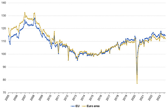
Figure 1.
Construction production in EU and Euro area showing cyclical nature of the construction activity; source: adapted based on the Eurostat data; note: index 2015 = 100 (vertical y-axis does not start at 0), calendar and seasonally adjusted data (code:sts_copr_m), 2005–2023.
In addition, the OECD and other statistical agencies have compiled information on construction price indices and their uses. Eurostat’s information can serve as a valuable reference for understanding the use of these indices in an economic and construction sector analysis [30]. (3) Building permits (denoted as building_permits and “sts_cobp_q” in Eurostat database) can be seen as a leading indicator of construction activity. An increase in building permits often precedes an increase in construction activity, making it an important variable for studying the phase shift of construction activity relative to the broader economy [29]. (4) The operating time ensured by the current backlog in construction (denoted as Construction_Operating_Time_by_Backlog or “ei_bsbu_q_r2” in the Eurostat database). It provides insight into the backlog of construction projects and is important for the analysis of construction activity in the context of broader economic conditions [31]. In addition, Lovell [32] discusses the importance of having a healthy backlog, the potential issues of having too long a backlog, and how to calculate a construction backlog using a work in progress (WIP) report [33]. Scalisi [34] explains that a company’s backlog is the amount or value of projects that they have in the pipeline on which work has not yet started. It also provides strategies for managing the backlog effectively [34].
The selection of these variables is important for examining the lag between the broader economy and construction activity for the following reasons: Construction production reflects the activity of the construction sector and provides an insight into the current state of the construction industry. The usefulness of up-to-date short-term business statistics, especially for market services and construction, including a production index for construction, has been highlighted by researchers in the literature [35]. The European construction sector accounts for more than 5% of gross value added, indicating its considerable economic importance [30]. The production index for construction is an important tool for tracking the output of the sector and its contribution to the overall economy. Overall, the production index for construction is a fundamental measure that provides insights into the short-term dynamics, cyclical patterns, and economic importance of the construction sector. Its role as a business cycle indicator and its contribution to economic planning and market research underline its importance in both academic and industrial contexts. Building permits, in turn, act as a leading indicator, signaling future construction activity. An increase in building permits often precedes an increase in construction activity, making it critical to understand the timing of construction activity relative to the broader economy [7,29]. Construction operating time by backlog provides information on the backlog of construction projects, which is important for analyzing construction activity in the context of broader economic conditions [31,32,33,34,35,36].
These variables are essential to understanding the relationship between construction activity and the broader economy, as they provide insight into the current status, future trends, and backlog of construction projects, allowing for a comprehensive analysis of the construction sector in relation to overall economic conditions. The selection of these variables is important for studying the lag between the broader economy and the construction activity because it allows for the analysis of how changes in the broader economy affect the construction sector over time. Changes in GDP can be expected to lead to changes in demand for construction services, which can be reflected in changes in construction production, building permits, and construction operating time by backlog.
In this study, GDP growth is used as a trailing average from the last four quarters, which holds scientific merit, particularly in addressing the challenges posed by the inherent volatility of quarterly changes. The decision to use a trailing average serves to mitigate the noise and short-term fluctuations present in the raw quarterly GDP growth data. By smoothing out these variations, the trailing average provides a more stabilized and representative measure of the underlying economic trends over a longer time frame. This approach aligns with the goal of capturing the sustained and meaningful patterns in the relationship between GDP growth and construction activity. Furthermore, the use of a trailing average allows for the identification of more enduring trends and facilitates the detection of significant correlations that may be obscured by the noise present in individual quarterly observations. Overall, this variable selection strategy enhances the robustness and reliability of the analysis by emphasizing the more persistent aspects of the economic dynamics under investigation.
3. Results
3.1. EU Countries (Panel Data Analysis)
The correlation between GDP growth and construction activity proxies is a nuanced interplay that transcends national boundaries. The analysis presented in this study, which is based on the cross-correlation function (CCF) approach, examines the positive lag max and negative lag max between GDP growth (trailing average) and key indicators of construction activity, namely construction production, building permits, and construction operating time by backlog, across different European countries. In particular, the positive lag max results converge within a narrow range (and specifically for the construction production variable), while the negative lag max shows interesting variations, highlighting the complex dynamics shaping these economic relationships (see Table 1 and Table 2 below). The CCF approach is used to identify when movements in construction occur in response to changes in the economy.

Table 1.
Cross-correlation results for positive lag max (GDP growth vs. construction indicators).
Table 2.
Cross-correlation results for negative lag max (GDP growth vs. construction indicators).
The positive lag max results shown in Table 1 reveal a remarkable uniformity across countries, with the majority possessing lags between 10 and 11 quarters (for construction production). This uniformity suggests a harmonized responsiveness of the construction sector to broader economic changes. For example, Denmark, with the lowest positive maximum lag of 9 quarters, and Poland, with the highest at 11 quarters, both suggest a delayed but synchronized response (see Figure 2).
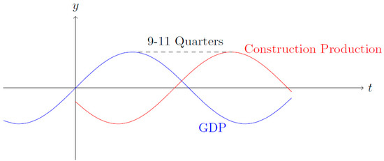
Figure 2.
Harmonized responsiveness of the construction sector to broader economic changes. Source: own elaboration.
This common pattern can be attributed to systemic factors such as construction market structures and the intrinsic nature of the construction industry. However, a more complicated story emerges when examining the CCF for GDP growth and building permits. Here, the positive lag max shows a wider range, ranging from 1 quarter for Ireland to 18 quarters for Belgium (although the latter is not a statistically significant result). This divergence prompts a critical examination of the factors influencing this variability. For example, the rapid response observed in Ireland may be related to a proactive regulatory environment that streamlines the approval process. Conversely, the long positive lag in Belgium may be indicative of bureaucratic hurdles or market complexities that cause delays in the approval phase. Such divergences underscore the need for local policy interventions and industry adjustments to ensure a more synchronized response between economic growth and construction permitting. Some interesting results emerge from the analysis of the CCF for GDP growth and construction operating time by backlog. The maximum positive lag ranges from 4 quarters (Ireland) to 21 quarters (the Czech Republic and Romania), representing a considerable spectrum of economic behavior. This wide variation challenges conventional assumptions about the temporal relationship between GDP growth and the dynamics of construction operating time. For example, Ireland’s rapid turnaround suggests efficient operational processes, while the extended positive lag in the Czech Republic or Romania suggests a more deliberate or targeted approach, possibly influenced by market size or regulatory complexity.
Overall, the positive lag max results suggest a synchronized response of the construction sector across European countries, albeit with nuanced differences. The positive lag max for building permits and construction time by backlog adds a layer of complexity, reflecting different national contexts and market specificities. This analysis calls for a shift from a one-size-fits-all approach to nuanced, localized strategies that take into account the unique economic landscapes that shape the construction industry in each country. Policymakers, industry leaders, and researchers can use these insights to design targeted interventions and foster more resilient, adaptive construction sectors in Europe’s dynamic economic landscape.
The cross-correlation function approach also highlights the negative maximum lag between GDP growth and the same key construction indicators across European countries. Table 2 unfolds a narrative of heightened heterogeneity, revealing the varied responses of the construction sector to broader economic shifts. This exploration seeks to unravel the nuances inherent in the negative lag max results, ultimately revealing an insightful metric that helps to understand the temporal linkages between the broader economy and the construction sector.
The negative lag max values presented in Table 2 offer a compelling narrative of the temporal dynamics between construction activity measures and changes in the broader economy. These negative lag max values signify the duration at which construction indicators precede shifts in GDP growth, establishing them as early indicators or harbingers of economic changes. An examination of the negative lag max values for construction production, building permits, and construction operating time by backlog across various countries reveals noteworthy patterns. The high negative lag max values across countries, coupled with strong negative correlations, underscore the synchronized role of the construction sector as a harbinger of changes in the broader economy. In the case of construction production, several countries show extended negative lags, indicating that fluctuations in construction output precede changes in GDP growth. For example, Austria, Romania, and Slovakia have negative max lags of 19–20 (and even Germany with its 18 quarters’ negative lag max), suggesting that construction production in these countries tends to signal economic changes well in advance. This just shows that the construction sector is very cyclical.
Building permits also prove to be a robust harbinger of economic changes, suggesting that changes in building permit issuance anticipate changes in GDP growth. Finland, with a negative lag max of 5, indicates that the permitting phase tends to signal economic changes five quarters ahead. The negative lag max values for construction operating time by (order) backlog further underline the anticipatory role of the construction sector. In particular, Estonia, France, Ireland, Latvia, Romania, and Slovenia have significant negative lag values, highlighting that construction operating times precede broader economic changes. For example, Estonia’s negative maximum lag of 21 indicates that operating time by order backlog tends to signal economic changes 21 quarters in advance.
It is important to note that negative lag max can be used to proactively manage the construction sector, as it signals economic changes ahead of time. This early signaling provides policymakers, industry stakeholders, and researchers with valuable insights into the upcoming economic climate. It allows for timely adjustments to strategies, interventions, and policies, fostering a more resilient and adaptive economic environment. Overall, the negative lag max results in Table 2 underscore that measures of construction activity proxies serve as harbingers that precede changes in the broader economy. Whether in the production phase, permitting processes, or operational schedules, the construction sector demonstrates a proactive role in signaling economic shifts. Recognizing this anticipatory nature enhances our understanding of the intricate linkages between the construction sector and the broader economy, providing a valuable tool for informed decision making. The negative lags, along with their interpretations, serve as an important guide for policymakers navigating the complex landscape of economic dynamics.
A CCF analysis, a powerful tool for identifying temporal correlations, serves as the starting point. By examining the timing and strength of the correlations between GDP growth and proxies for construction activity (construction production, building permits, and construction operating time by backlog), light is shed on the intricate patterns that govern their relationships. A deeper level of understanding emerges when moving to the Toda–Yamamoto causality tests presented in Table 3.
Table 3.
Toda–Yamamoto test for causality (lag order equal to the positive lag max).
The Toda–Yamamoto tests aim to determine whether lagged GDP growth can be considered a driving force behind changes in the construction sector. The directional nature of the causality tests adds a crucial layer to the analysis, providing insights beyond the indication of the temporal offset at which the correlation between GDP growth and various proxies for construction activity (such as construction production, building permits, and construction operating time by backlog) is maximized.
Interpreting the results from Table 3, it is clear that causality is confirmed to varying degrees for different countries and construction activity proxies. The majority of countries show causality for GDP growth and at least one of the construction activity proxies. On the contrary, there are only four EU countries (i.e., Bulgaria, Ireland, Malta, and Poland) that show no causality for any of the construction activity proxies (at the lag order indicated in the CCF analysis results). This nuanced pattern highlights the multifaceted nature of the relationship between GDP growth and construction activity across different economic landscapes. An interesting observation emerges when looking at Italy and Portugal, where causality is confirmed for all three construction activity proxies at the lag order corresponding to positive lag max. This suggests a more consistent and pronounced influence of GDP growth on construction activity in these countries, adding a layer of complexity to the overall analysis. Going beyond Table 3, the causality tests in Table A4 presented in Appendix A provide a detailed breakdown of the lag orders at which causality is confirmed. In general, for GDP growth and all three construction activity proxies, causality tends to be confirmed at lower lag orders (1–4 quarters) and in the mid-to-late teens (15–18 quarters). This pattern suggests that changes in GDP growth have both short- and medium-term effects on these construction activity proxies.
More specifically, the Toda–Yamamoto causality tests presented in Table A4 (presented in Appendix A) offer valuable insights into the temporal dynamics between GDP growth and various construction activity proxies across European countries. It shows the lag orders at which causality is confirmed for construction production, building permits, and construction operating time by backlog, shedding light on the nuanced relationships between these variables. One notable pattern that emerges is the variability in the lag orders at which causality is confirmed. For construction production, countries such as Austria, Croatia, Denmark, Estonia, Finland, Germany, Italy, Latvia, Lithuania, Luxembourg, Portugal, and Sweden exhibit causality for the lag order corresponding to the Positive Lag Max indicated in the CCF analysis. Also, when testing causality for a whole range of lag orders (from 1 to 20), the majority of EU countries exhibit causality across a broad spectrum of lag orders, ranging from the early stages (1–4) to mid and late teen numbers (15–18). This diverse pattern suggests a complex and multifaceted interplay between GDP growth and construction production across different nations.
For building permits, the number of lags at which causality is confirmed is smaller than for construction production. In the case of the majority of countries, however, causality is confirmed at various lag orders, often within the first four quarters. Only in three cases (Austria, Belgium, and Germany), causality is confirmed only for values of lag order from the upper range of the tested set of lag values (meaning non-immediate or delayed influence). The low value of the lag order implies a robust and relatively immediate influence of GDP growth on building permit issuance in these countries. The same interpretation as with construction production and building permits is with the construction operating time by backlog. Apart from France and Ireland, the rest of the countries show significant causality with both lower and upper lag order (which is indicative for immediate and delayed response of the GDP growth changes). However, the results’ variability suggests a less uniform relationship between GDP growth and construction operating time by backlog, emphasizing the need for localized analyses and strategies. The logical interpretation of these lag patterns underscores the intricate dynamics between GDP growth and the construction sector. Construction production, in particular, exhibits a more consistent pattern across several countries, indicating a robust influence of GDP growth across different timeframes. In contrast, building permits and construction operating time by backlog display mixed patterns, suggesting a less consistent relationship with GDP growth.
Scientifically, these findings imply that the influence of GDP growth on construction activity varies not only between countries but also across different facets of the construction sector. However, the immediate response observed in all construction activity proxies signifies a proactive and synchronized adjustment to economic changes in numerous European nations. However, the mixed patterns when it comes to specific countries (like Austria, Belgium, Germany, France, Ireland) and building permits or construction operating time by backlog highlight the complex and context-dependent nature of these relationships. Importantly, these causality results from Table 3 and Table A4 (presented in Appendix A) do not diminish the value of the earlier cross-correlation function (CCF) analysis, particularly the positive lag max and correlation lag max results. The CCF analysis provided a broader understanding of the synchronized response of the construction sector to GDP growth across European countries. The Toda–Yamamoto tests, while offering insights into specific lag orders, complement this understanding by revealing the nuanced and variable nature of the causality relationships. In conclusion, the Toda–Yamamoto causality tests enrich our understanding of the temporal linkages between GDP growth and construction activity proxies. The variable patterns observed highlight the importance of localized analyses and underscore the need for policymakers, industry stakeholders, and researchers to consider the unique economic landscapes shaping the construction industry in each country. The combination of the CCF analysis and causality tests provides a comprehensive framework for informed decision making in navigating the intricate interplay between economic growth and the construction sector.
In addressing the question of why it is worthwhile to test causality primarily from lagged GDP growth to construction proxies, there is an alignment with economic theory that can be indicated. Lagged GDP growth serves as a leading indicator, reflecting changes in the broader economic landscape. Testing the reverse causality, where construction proxies cause GDP growth, holds less value, as construction activities are often viewed as early indicators rather than drivers of economic changes. The confirmation of causality at multiple lag orders, as seen in Table A4 (presented in Appendix A), indicates that the impact of GDP growth on construction activity proxies is complex and spans various timeframes. This complexity is reflective of the dynamic nature of the relationship between economic growth and the construction sector. All in all, the combined insights from the CCF analysis and Toda–Yamamoto causality tests offer a comprehensive understanding of the intricate dynamics between GDP growth and construction activities. The variations across countries, the nuanced patterns in lag orders, and the consistent influence observed in specific countries contribute to a rich tapestry of knowledge for policymakers, industry stakeholders, and researchers navigating the interplay between the construction sector and the broader economy. Rather than diminishing the value of a CCF analysis, causality tests complement it, providing a more holistic view and paving the way for a deeper exploration of the economic forces shaping our built environment.
3.2. Poland
Examining the results for Poland, particularly through the lens of the CCF analysis and the Toda–Yamamoto test for causality, is crucial due to Poland’s unique socio-economic landscape and its dynamic position within the European Union. As a country that has undergone significant economic transformations, understanding the intricate relationships between GDP growth and the construction sector provides valuable insights for policymakers. Poland’s resilience during global economic crises, such as the 2009–2010 financial downturn, demonstrates its capacity for adaptive economic strategies. By exploring the lagged dynamics between GDP growth and construction activity proxies, this study becomes a nuanced guide for crafting tailored policies that resonate with Poland’s specific economic cycle pattern, reinforcing its role as a forerunner for strategic decision making in the broader EU context.
In the light of the CCF results presented in Table 1 and Table 2, Polish construction production turns out to be a synchronized companion of GDP growth, responding both positively and negatively to economic shifts. The positive correlation, which is particularly significant with an 11-quarter lag, implies that an upturn in GDP growth precedes a subsequent increase in construction production. In turn, the negative correlation with a 21-quarter lag signals a decline in GDP growth following a decline in construction production (although the result is not statistically significant). This intertwined relationship underscores the responsiveness of the construction sector to broader economic trends, providing a robust basis for forecasting and strategic planning. Practical implications are that these findings can help improve strategic planning and adaptability. Policymakers and construction firms can strategically plan for future construction demand based on expected changes in GDP. In terms of adaptability, understanding the synchronized response allows for agile adaptation to economic fluctuations, thereby increasing resilience. In turn, building permits can be considered a moderate leading indicator. While showing a positive correlation, building permits have a more nuanced relationship with GDP growth, as the correlation lag max is much lower compared to construction production. The positive correlation, which is significant with a lag of 12 quarters, suggests that an increase in GDP growth precedes a subsequent increase in building permits. With respect to the construction operating time by backlog, both positive and negative correlations that are not statistically significant indicate a weak relationship. The positive correlation (which is almost close to zero) with a lag of 11 quarters suggests a very weak relationship between GDP growth and construction operating time by backlog. Similarly, the negative correlation with a lag of six quarters indicates a weak relationship between GDP growth and construction operating time by backlog. This indicator may not serve as a reliable predictor of changes in the Polish construction market. Policymakers and construction managers should interpret this indicator with caution, as it is moderately leading (correlation lag max is positive although it is almost close to zero) and yet the result of the positive lag max is statistically insignificant. Caution is also warranted when forecasting. Construction operating time by backlog can provide a glimpse of future construction activity, but an insignificant lag and weaker correlation require careful consideration in long-term forecasting. Therefore, construction operating time by backlog can be used in conjunction with other indicators for a more complete understanding (can be used as a complementary analysis), as it has limited predictive power for Poland. Given the lack of statistical significance, caution should be exercised when considering construction operating time by backlog as a predictive tool. Policymakers and industry stakeholders may need to explore alternative indicators to more accurately reflect the dynamics of the construction market. It is also worth noting the consistency of positive lag max values for all three measures of construction activity (i.e., for construction production, building permits, and construction operating time by backlog—11, 12, and 11, respectively), which underscores the reliability of these results. Figure 3 shows the CCF for GDP growth and various proxies for construction activity (for Poland).
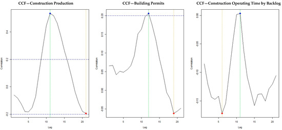
Figure 3.
CCF for GDP growth and different construction activity proxies (for Poland); note: green and yellow dotted lines indicate the positive and negative lag max, respectively. The blue dot represents the maximum positive correlation for the value of the maximum positive lag, while the red dot represents the maximum negative correlation for the value of the maximum negative lag. Source: own elaboration in R-Studio.
The Toda–Yamamoto test for causality in Poland, as detailed in Appendix A Table A4, reveals distinctive patterns of causality between various proxies for construction activity and the broader economy. In particular, Poland stands out among four EU countries, including Bulgaria, Ireland, and Malta, by showing a lack of causality at the lag orders identified in the results of the CCF analysis. Contrary to the positive lag max order indicated by the CCF analysis, the Toda–Yamamoto test reveals causality for construction output at lag orders 1, 2, 6, and 7. Similarly, for building permits, causality is confirmed at lag orders 17, 18, 19, and 20, which differs from the CCF results. Construction operating time by backlog shows causality for Poland at lag orders 5, 20, and 21. This nuanced causality pattern underscores the complexity of the relationship between construction activity and economic shifts in Poland, which warrants a more in-depth examination of lag dynamics for precise policy considerations and strategic planning. The nuanced causality results in Poland, as evidenced by the Toda–Yamamoto test, require a strategic reassessment by policymakers. Given the different lag orders for causality in different construction proxies, a tailored approach is essential. For construction production, policymakers could implement a short-term fiscal stimulus or targeted investment incentives to capitalize on the immediate positive feedback loop. In contrast, for building permits, a more forward-looking strategy is recommended, involving streamlined regulatory processes and proactive engagement with developers to foster a conducive environment for future projects. For construction backlogs, real-time monitoring mechanisms and flexible policies that can respond to short-term economic changes would be critical.
In terms of recommendations for strategic decision making based on the results presented in Table 1 and Table 2, it makes sense to focus on the construction production variable. With its consistently significant correlations, construction production stands out as a reliable indicator for long-term forecasting and strategic decision making. Although informative, building permits should be treated with caution due to their lower correlation value (Corr. Pos. Max). Given the limited predictive power of construction operating time by backlog, the exploration of alternative indicators is crucial for a more comprehensive understanding of the construction market. In navigating the dynamic interplay between GDP growth and the construction sector in Poland, a nuanced interpretation of these indicators is essential. Armed with these insights, policymakers, construction managers, and researchers can make informed decisions that foster a resilient and adaptable construction sector in Poland’s ever-changing economic landscape.
4. Discussion
The results, based on the CCF analysis, unravel nuanced relationships between GDP growth and a number of construction activity proxies, providing insights into the economic synchrony between the broader economy and the construction sector in Poland and other EU countries. Examining construction production, building permits, and construction operating time by backlog reveals distinct patterns in the responsiveness of the construction sector in EU countries to broader economic changes. In this discussion, we explore potential sources of these results, highlighting the specificities of the construction sector, and conclude with recommendations and policy suggestions for authorities based on the findings.
In the broader context of EU countries, the study reveals interesting patterns that underline the role of country specificity in shaping the response of the construction sector to economic fluctuations. In particular, differences in the strength and timing of correlations between GDP growth and construction indicators across EU countries suggest the influence of several factors. The size and productivity of a country, as well as its orientation toward construction activities, emerge as potential determinants. This is in line with a study by Sun et al. [37], which provides insights into the factors that contribute to the variation in construction shares across countries. The study focuses on the performance of the construction sector and its impact on the overall economy, given its close interdependence with other sectors. The paper highlights the high elasticity between changes in the construction share and GDP growth, which is around 0.37–0.4 for advanced and central, eastern, and south-eastern European countries. The study also suggests that the size and productivity of a country, as well as its orientation toward construction activities, are potential determinants of the strength and timing of correlations between GDP growth and construction indicators [37]. Typically, larger economies have more complex and interconnected systems [38], affecting the lag and strength of the correlation. In addition, countries with a robust construction sector have different dynamics than those with a less construction-oriented economy [37]. Bureaucratic efficiency, highlighted in the context of building permits, plays a crucial role [39,40]. The different lags and correlation strengths can be attributed to differences in administrative procedures and regulatory frameworks across EU member states. Countries with streamlined and efficient permitting processes are able to respond more quickly to economic changes, leading to more immediate correlations. For example, Germany’s strong and efficient economy as an EU powerhouse contributes to a relatively shorter lag between GDP growth and construction production. The country’s construction-oriented approach and robust bureaucratic efficiency are factors influencing these results. In addition, countries with traditionally vibrant construction sectors, such as Spain and Italy, show more pronounced correlations, underscoring the economic importance of construction activities in these countries. It is also important to highlight the importance of bureaucratic procedures in obtaining building permits. Countries with more bureaucratic hurdles may experience longer lags (e.g., Estonia, Lithuania, or Romania), which affects the immediacy of the correlation between GDP growth and construction indicators.
The synchronized response of construction production in Poland to GDP growth, both positively and negatively, suggests a robust linkage between economic conditions and construction production. The positive correlation, particularly significant with an 11-quarter lag, implies that an upturn in GDP growth precedes a subsequent increase in construction production. This pattern may be attributed to the nature of construction projects, often characterized by long planning and development phases [7,19]. Delays in project initiation due to economic uncertainties during downturns might contribute to the observed lag in construction production recovery [19]. Conversely, the negative correlation with a 21-quarter lag signals a decline in GDP growth following a decrease in construction production. This could reflect the cyclical nature of the construction sector, with reductions in construction projects during economic downturns leading to a subsequent decline in GDP growth.
The construction industry’s sensitivity to economic fluctuations is well documented, and Poland’s case aligns with global trends [1,3,4,41,42]. The lag dynamics observed are also influenced by factors such as funding availability, regulatory processes, and the intricate interplay between private and public construction projects [7,41]. Policymakers and industry leaders can leverage these insights to anticipate construction trends and plan interventions that stimulate construction activity during economic downturns.
Building permits in Poland display a moderately leading role, with a positive correlation that becomes significant for a lag of 12 quarters. This delayed response may be indicative of the bureaucratic complexities and regulatory processes inherent in obtaining building permits. The planning and approval stages of construction projects often involve multiple stakeholders, and the observed lag reflects the time required for these processes to unfold. Policymakers should consider streamlining and expediting building permit approval procedures to enhance their effectiveness as leading indicators. In addition, caution should be exercised in relying solely on building permits for long-term forecasting, as the low correlation value calls for a more comprehensive approach using multiple indicators.
The weak and statistically insignificant correlation between GDP growth and construction operating time by backlog in Poland underscores the limited predictive power of this indicator. The positive correlation with an 11-quarter lag indicates a very weak relationship between increased GDP growth and increased construction operating time by backlog. Similarly, due to the lack of statistical significance, the negative correlation with a six-quarter lag suggests a weak relationship between GDP growth and construction operating time by backlog. This may be attributed to the intricate nature of construction project timelines, which are influenced by factors such as project size, complexity, and contractual arrangements. Given the lack of statistical significance, policymakers and industry stakeholders should explore alternative indicators to gain a more accurate understanding of the construction market dynamics. The consideration of factors affecting construction operating time, such as project management efficiency, contractual flexibility, and market demand, can contribute to the development of more reliable predictors for construction activity.
Based on the above, the following recommendations and policy implications can be suggested: (1) Improvement in regulatory efficiency of building permits. Authorities should focus on streamlining and expediting the building permit approval process to strengthen its effectiveness as a leading indicator. Reduced bureaucracy and increased transparency in regulatory processes can contribute to more timely and reliable signals of construction activity. (2) Investment in infrastructure projects during economic downturns. Given the lagged response of the construction sector to changes in GDP, policymakers should consider strategically investing in infrastructure projects during economic downturns to stimulate construction activity. This countercyclical approach can contribute to economic recovery and job creation. (3) The promotion of industry collaboration and innovation. Encouraging public–private collaboration and promoting innovation in construction technologies can improve the industry’s adaptability [7,43]. Public authorities can encourage research and development in construction methods that reduce project times and costs, ultimately contributing to a more resilient construction sector. (4) The diversification of stimulus measures. Policymakers should take a diversified approach to a stimulus during downturns, taking into account the specificities of the construction sector. Targeted incentives for construction projects, including tax breaks and financing support, can accelerate recovery and strengthen the contribution of construction to economic growth. (5) Continuous monitoring and adaptive planning. Given the cyclical nature of the construction sector, authorities should implement continuous monitoring of economic indicators and construction activity. This adaptive planning approach allows for timely adjustment of policies and interventions in line with the dynamic economic landscape.
All in all, the nuanced dynamics between GDP growth and the construction sector in Poland necessitate targeted interventions and a deep understanding of the sector’s specificities. Policymakers and industry stakeholders can leverage these findings to formulate adaptive strategies that enhance the resilience and responsiveness of the construction industry, contributing to sustainable economic development.
It is important to note that construction serves as a major contributor to the business cycle, reflecting macroeconomic activity in a unique manner [44,45,46,47]. It is important to remember that the construction sector is not homogeneous and there are different subsectors within the sector as a whole, i.e., residential, commercial, infrastructure, and industrial, which exhibit different cyclical patterns [7,48]. The dynamics within the construction sector are influenced by competition for inputs such as land, labor, and capital. For example, construction spending, which reflects total investment in real estate, shows that both commercial and residential spending followed similar trajectories until 2001 (as shown in Figure 4).
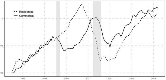
Figure 4.
Differences between commercial construction spending and residential construction spending; source: https://data.gov/ accessed on 5 December 2023. Note: The gray area indicates the timing of the turning point in the economic cycle, i.e., when a recession occurred in the broader economy.
Post-2001, especially after recession periods, their behaviors diverge, indicating significant differences in cyclical patterns tied to macroeconomic fluctuations [49]. Interplays between residential and commercial real estate are evident in property prices and real estate investment [18,50]. Co-movements during crises, such as the 2009–2010 financial crisis, display sharp falls followed by gradual recoveries, emphasizing the interconnected nature of these sectors [51,52]. Recent shifts, like the move to remote work due to the COVID-19 pandemic, underscore the need to understand the mechanisms governing these real estate co-movements [53]. Empirical relationships between residential and commercial real estate are explored, highlighting substitution between the two sectors [54,55]. The introduction of the construction sector into a DSGE model captures the competition for inputs and real estate between different segments of producers [9,15]. Positive housing preference shocks impact demand for residential real estate, influencing commercial structures’ production costs and reducing demand by companies, leading to the real estate substitution channel. This mechanism plays a crucial role in understanding the dynamic fluctuations in real estate investment over the business cycle [53,56]. The historical decomposition reveals the driving forces behind movements in the real estate market, emphasizing the co-movement of commercial and residential real estate investment during the financial crisis [15,56]. The fall in overall supply following the financial crisis offset some of the demand-driven price changes, showcasing the intricate relationship between the broader economy and the construction sector.
There are certain issues that are crucial to understanding the subject of this study, namely government intervention and market fluctuations [7,48], the impact of the COVID-19 pandemic [57], lessons for residential construction policies [7,58,59,60,61,62], central bank policies [63,64], the role of business cycles, and the necessity of economic crises [7,48]. Another important issue is the significant impact of government intervention, particularly by the NBP, in influencing the real estate market. NBP policies, including interest rate adjustments and credit accessibility, emerged as key drivers of market fluctuations. This phenomenon is consistent with the findings of previous research where central bank policies have been identified as powerful tools for managing economic conditions [63]. While it is recognized that the primary responsibility of any central bank is to ensure price stability, it is also important to maintain a balanced policy [63]. The NBP’s actions resulted in exceptionally low interest rates, which translated into favorable credit conditions and had a significant impact on the dynamics of the construction market [65]. However, a closer examination of the balance between price stability and the needs of the construction market is recommended.
It is worth noting the impact of external shocks on the residential construction sector. The impact of the COVID-19 pandemic on the residential construction market was profound [57,63]. While reduced developer activity and lower demand for housing due to the pandemic were widespread, there is evidence that the crisis also stimulated interest in residential real estate. Sobieraj and Metelski [57] found that interest rate cuts and the availability of fixed-rate mortgages led to significant price increases in 2020 and early 2021. The study of the evolution of the business cycle provides an opportunity to critically assess residential construction policies. In particular, it shows that economic crises are an inherent part of market cycles and play a cleansing role in the sector. The evolution of construction activity over the period 2000–2023 in Poland confirms the sensitivity of the construction sector to economic fluctuations. This is in line with general economic theory, which suggests that construction markets are pro-cyclical [3]. The data presented support the notion that during periods of economic prosperity, the construction sector (and especially residential construction) experiences increased demand and price growth. However, these trends are reversed during economic downturns. While crises can be disruptive, they also play a crucial role in cleansing markets and restoring healthy competition [66]. Therefore, business cycles should be seen as natural phenomena with their own ebb and flow.
It is also worth noting that construction projects go through different phases and stages, and planning the construction processes is crucial to avoid the prolongation or failure of individual phases and the whole project [7,19,48]. Forecasting business cycles is therefore an important factor to consider when managing construction projects. Business cycles refer to the overall state of the economy as it moves through four stages in a cyclical pattern: the expansion, peak, contraction, and trough [67,68,69]. The alternating phases of the business cycle are expansions and contractions (also known as recessions) [70]. The construction sector tends to lag behind the general business cycle at both the trough and the peak [2,3,42]. There is some scientific evidence that shows the importance of incorporating business cycle forecasting into the management of construction projects: (1) Surviving business cycles. Managing business cycles can help companies plan strategically to protect themselves from impending downturns and position themselves to take maximum advantage of economic expansions [67]. (2) Avoiding expansion during a recession. If a construction company follows the rest of the economy, warning signs of an impending recession may suggest that it should not expand its activity. It may be better to build up its cash reserves [67]. (3) Identifying the phases of the business cycle. The duration of business cycles varies, making it difficult to time the phases. However, identifying the phases of the business cycle can help investors position their investments to take advantage of different phases [2]. Therefore, it is essential to take into account the economic cycle forecast when planning construction processes in order to avoid the prolongation or failure of individual phases and the entire project [2]. To conclude, economic forecasting is crucial for the management of a construction project in order to avoid failures in the management of its various phases. It is essential to take into account the economic cycle forecast when planning construction processes in order to avoid the prolongation or failure of individual phases and the whole project.
Analyzing the historical business cycle of the Polish construction industry from 2001 to 2022 provides valuable insights into the sector’s dynamics and its intricate relationship with economic fluctuations [7,48]. The cyclical patterns, as outlined in Table 3, underscore the sector’s vulnerability to market phenomena, government policies, and global conditions.
The recovery from the 2009–2010 financial crisis, taking about three years, aligns with the observed positive lag max in the cross-correlation function (CCF) results for both the broader economy, reflected in GDP growth, and construction activity, particularly construction production, with a lag of 11 quarters [59,61,62,63]. Economic uncertainties during downturns lead to postponed or canceled projects, reduced capital spending, and a direct impact on the construction sector [19]. The sector’s close link to the real estate market exacerbates its vulnerability, as declining real estate values make developers cautious and delay new projects [7]. The COVID-19 pandemic further emphasized the sector’s unique vulnerability, accentuating delays in its recovery due to prolonged planning phases and close ties to real estate dynamics [53,57,63,64].
Real estate policy emerges as a pivotal factor shaping the Polish construction sector’s response to economic fluctuations [7,71,72,73]. Government interventions, exemplified by events in 2006 post Poland’s EU accession, underscore the profound impact on the construction sector and the broader economy [74]. The positive lag max value in CCF for construction production at 11 quarters aligns with government policy changes during this period, including the abolition of tax deductions and the non-extension of the reduced VAT rate, triggering a surge in construction demand and subsequent housing crisis [74,75].
Understanding the cyclical nature of the construction market requires a comprehensive examination of various economic factors, including lending rates, the central bank reference rates, client savings, and migration data. Recognizing the dynamic interplay of these elements with construction activity is crucial for constructing informed forecasts and resilient policies. The detailed historical overview provides valuable context for interpreting the CCF results, emphasizing the need for nuanced policy considerations and future improvements to enhance economic resilience [7,63,74].
5. Conclusions
This study examines the multifaceted relationship between the business cycle and the construction sector in EU countries, with a special focus on Poland. Using the cross-correlation function (CCF) and causality tests (i.e., the Toda–Yamamoto test), and analyzing a comprehensive dataset covering the period from 2000Q1 to 2023Q2 for 27 EU countries, the research unravels nuanced temporal patterns that shed light on the construction sector’s lagged response to shifts in GDP growth.
The background to the study is the recognition of the construction sector’s unique sensitivity to economic fluctuations and its significant impact on the overall business cycle [1,4,5]. The dynamic interplay between GDP growth and proxies for construction activity, including construction production, building permits, and construction operating time by backlog, is carefully examined. In particular, the positive lag max results for construction production show a synchronized response across European countries, with lags predominantly between 10 and 11 quarters. This implies a harmonized response of the construction sector to broader economic changes. Conversely, the positive lag max results for building permits and construction time by backlog show greater variation, underscoring the need for nuanced, localized strategies.
The study’s robustness is underpinned by its ability to quantitatively analyze the temporal dynamics between the business cycle and the construction sector, providing a rigorous foundation for the research. The positive correlation with an 11-quarter lag between GDP growth and construction production in Poland highlights the sector’s robust link to economic conditions, suggesting that an upturn in GDP precedes a subsequent increase in construction production. However, the negative correlation with a 21-quarter lag signals a decline in GDP growth following a decline in construction production, underlining the cyclical nature of the construction sector.
The recommendations derived from the study have practical implications for policymakers and industry stakeholders. Streamlining and accelerating building permit approval processes are suggested to enhance their effectiveness as leading indicators, particularly in Poland, where building permits exhibit a moderate leading role with a positive correlation that becomes significant with a lag of 12 quarters. Policymakers are also encouraged to strategically invest in infrastructure projects during economic downturns, given the construction sector’s lagged response to changes in GDP.
The significance of the study lies in its contribution to a nuanced understanding of economic synchrony and its potential to shape strategies for sustainable economic development. However, further avenues for the continuation of this research can be explored by conducting additional studies to quantify the impact of the variables studied. For example, the use of VAR models could help to better understand the relationships and dynamics within the construction sector and its interaction with the broader economy. For example, researchers can explore cross-country spillover effects, identifying potential transmission channels and shared economic trends. This approach could provide a comprehensive understanding of how economic shocks or policy changes in one country reverberate across the construction sectors of other countries. In addition, VAR models offer the flexibility to incorporate multiple economic indicators simultaneously, allowing for a more nuanced examination of the multifaceted relationships between GDP growth and construction activity. Applying the VAR methodology to such an extensive dataset as the one used in this study has the potential to uncover intricate patterns and contribute to a more holistic understanding of the global economic synchronicity with the construction sector. In addition, exploring the impact of external shocks, such as the COVID-19 pandemic, on the construction sector and reassessing the balance between price stability and the needs of the construction market in light of government interventions could be fruitful areas for future research. Overall, this study serves as a valuable foundation for advancing our understanding of the temporal dynamics between the business cycle and the construction sector, thereby laying the groundwork for informed decision making in the areas of policymaking and industry strategy.
Author Contributions
Conceptualization, J.S.; methodology, J.S. and D.M.; validation, J.S.; investigation, J.S. and D.M.; resources, J.S.; data curation, D.M.; writing—original draft preparation, J.S. and D.M.; writing—review and editing, J.S. and D.M.; visualization, D.M.; supervision, J.S. All authors have read and agreed to the published version of the manuscript.
Funding
This research received no external funding.
Data Availability Statement
The data used in the study, i.e., Gross Domestic Product (GDP) growth (in the Eurostat database under the symbol: “namq_10_gdp”), the construction production (in the Eurostat database under the symbol: “sts_copr_q”), building permits (in the Eurostat database under the symbol: “sts_cobp_q”) and the operating time ensured by the current construction backlog (in the Eurostat database under the symbol: “ei_bsbu_q_r2”) are publicly available and have been downloaded from the Eurostat database: https://ec.europa.eu/eurostat/data/database.
Conflicts of Interest
The authors declare no conflicts of interest.
Appendix A
Table A1.
GDP growth (trailing average) and construction production (trailing average).
Table A1.
GDP growth (trailing average) and construction production (trailing average).
| Country | Lag Positive Max | Corr. Positive Max | Significance, Positive | Lag Negative Max | Corr. Negative Max | Significance, Negative |
|---|---|---|---|---|---|---|
| Austria | 11 | 0.75034244 | TRUE | 19 | −0.3738843 | TRUE |
| Belgium | 10 | 0.64267612 | TRUE | 5 | −0.2871945 | TRUE |
| Bulgaria | 11 | 0.71368833 | TRUE | 3 | −0.1316561 | FALSE |
| Croatia | 11 | 0.65926824 | TRUE | 21 | 0.16432097 | FALSE |
| Cyprus | 10 | 0.68333352 | TRUE | 1 | 0.02799514 | FALSE |
| Czechia | 11 | 0.62189964 | TRUE | 6 | −0.1915008 | FALSE |
| Denmark | 9 | 0.82618713 | TRUE | 1 | −0.1678132 | FALSE |
| Estonia | 11 | 0.80656698 | TRUE | 2 | −0.4859713 | TRUE |
| Finland | 10 | 0.80126279 | TRUE | 3 | −0.4295581 | TRUE |
| France | 10 | 0.75161016 | TRUE | 5 | −0.3379367 | TRUE |
| Germany | 10 | 0.62509243 | TRUE | 18 | −0.4532963 | TRUE |
| Greece | 11 | 0.60575408 | TRUE | 1 | −0.162733 | FALSE |
| Hungary | 10 | 0.58793913 | TRUE | 4 | −0.1455338 | FALSE |
| Ireland | 10 | 0.67383478 | TRUE | 1 | −0.0377104 | FALSE |
| Italy | 10 | 0.7780398 | TRUE | 4 | −0.2834003 | TRUE |
| Latvia | 11 | 0.73798295 | TRUE | 1 | −0.5475307 | TRUE |
| Lithuania | 10 | 0.75643946 | TRUE | 3 | −0.3469586 | TRUE |
| Luxembourg | 10 | 0.46703173 | TRUE | 16 | −0.3008562 | TRUE |
| Malta | 9 | 0.19544072 | FALSE | 13 | −0.249064 | TRUE |
| The Netherlands | 10 | 0.75343036 | TRUE | 3 | −0.2112726 | TRUE |
| Poland | 11 | 0.534634 | TRUE | 21 | −0.1941327 | FALSE |
| Portugal | 11 | 0.68016029 | TRUE | 1 | −0.1567826 | FALSE |
| Romania | 10 | 0.45728038 | TRUE | 19 | −0.4011873 | TRUE |
| Slovakia | 11 | 0.72402075 | TRUE | 20 | −0.094215 | FALSE |
| Slovenia | 10 | 0.71754757 | TRUE | 3 | −0.1157093 | FALSE |
| Spain | 11 | 0.66274066 | TRUE | 1 | −0.132355 | FALSE |
| Sweden | 9 | 0.70350688 | TRUE | 16 | −0.5466544 | TRUE |
Table A2.
GDP growth (trailing average) and building permits.
Table A2.
GDP growth (trailing average) and building permits.
| Country | Lag Positive Max | Corr. Positive Max | Significance, Positive | Lag Negative Max | Corr. Negative Max | Significance, Negative |
|---|---|---|---|---|---|---|
| Austria | 17 | 0.22791016 | TRUE | 7 | −0.1146977 | FALSE |
| Belgium | 18 | 0.16046107 | FALSE | 7 | −0.1097223 | FALSE |
| Bulgaria | 10 | 0.52367045 | TRUE | 21 | −0.0290328 | FALSE |
| Croatia | 7 | 0.44112948 | TRUE | 21 | −0.1096242 | FALSE |
| Cyprus | 2 | 0.53098328 | TRUE | 21 | −0.132341 | FALSE |
| Czechia | 11 | 0.41418497 | TRUE | 21 | 0.09788257 | FALSE |
| Denmark | 12 | 0.45158535 | TRUE | 1 | −0.0732891 | FALSE |
| Estonia | 12 | 0.3033182 | TRUE | 21 | −0.2619799 | TRUE |
| Finland | 14 | 0.27693927 | TRUE | 5 | −0.2407054 | TRUE |
| France | 11 | 0.38881902 | TRUE | 21 | −0.2247474 | TRUE |
| Germany | 15 | 0.17950915 | FALSE | 4 | −0.0947647 | FALSE |
| Greece | 4 | 0.4958666 | TRUE | 21 | 0.17054023 | FALSE |
| Hungary | 5 | 0.40305581 | TRUE | 21 | −0.040497 | FALSE |
| Ireland | 1 | 0.30591193 | TRUE | 21 | −0.3724941 | TRUE |
| Italy | 2 | 0.40240938 | TRUE | 21 | 0.03002868 | FALSE |
| Latvia | 10 | 0.56279674 | TRUE | 21 | −0.3939313 | TRUE |
| Lithuania | 11 | 0.28265177 | TRUE | 20 | −0.3043274 | TRUE |
| Luxembourg | 13 | 0.11808563 | FALSE | 1 | −0.2060131 | TRUE |
| Malta | 8 | 0.17021196 | FALSE | 19 | −0.1747846 | FALSE |
| The Netherlands | 2 | 0.24788428 | TRUE | 21 | −0.0487801 | FALSE |
| Poland | 12 | 0.20576696 | TRUE | 19 | −0.0619062 | FALSE |
| Portugal | 2 | 0.29438377 | TRUE | 21 | 0.10170547 | FALSE |
| Romania | 8 | 0.21342109 | TRUE | 21 | −0.2742964 | TRUE |
| Slovakia | 7 | 0.17379266 | FALSE | 15 | −0.1506035 | FALSE |
| Slovenia | 8 | 0.3970357 | TRUE | 21 | −0.2498229 | TRUE |
| Spain | 9 | 0.4788713 | TRUE | 21 | 0.05619566 | FALSE |
| Sweden | 11 | 0.16087669 | FALSE | 20 | −0.1967492 | FALSE |
Table A3.
GDP growth (trailing average) and construction operating time by backlog.
Table A3.
GDP growth (trailing average) and construction operating time by backlog.
| Country | Lag Positive Max | Corr. Positive Max | Significance, Positive | Lag Negative Max | Corr. Negative Max | Significance, Negative |
|---|---|---|---|---|---|---|
| Austria | 10 | 0.2448259 | TRUE | 2 | −0.0948503 | FALSE |
| Belgium | 10 | 0.2853268 | TRUE | 2 | −0.1313232 | FALSE |
| Bulgaria | 20 | 0.3320451 | TRUE | 3 | −0.0663192 | FALSE |
| Croatia | 10 | 0.5672142 | TRUE | 4 | 0.1135489 | FALSE |
| Cyprus | 10 | 0.4942949 | TRUE | 21 | 0.0512263 | FALSE |
| Czechia | 21 | 0.2218827 | TRUE | 1 | −0.009933 | FALSE |
| Denmark | 9 | 0.4083496 | TRUE | 1 | −0.1445435 | FALSE |
| Estonia | 10 | 0.5488934 | TRUE | 21 | −0.4315475 | TRUE |
| Finland | 12 | 0.345124 | TRUE | 6 | −0.2645239 | TRUE |
| France | 11 | 0.2777531 | TRUE | 1 | −0.2901737 | TRUE |
| Germany | 11 | 0.3029154 | TRUE | 2 | −0.0684419 | FALSE |
| Greece | 5 | 0.3821312 | TRUE | 21 | −0.1051868 | FALSE |
| Hungary | 11 | 0.2905211 | TRUE | 17 | 0.025763 | FALSE |
| Ireland | 4 | 0.2558471 | TRUE | 18 | −0.1182239 | FALSE |
| Italy | 11 | 0.2525602 | TRUE | 1 | −0.3293829 | TRUE |
| Latvia | 10 | 0.386397 | TRUE | 19 | −0.3400909 | TRUE |
| Lithuania | 11 | 0.4954698 | TRUE | 20 | −0.2414501 | TRUE |
| Luxembourg | 20 | −0.035216 | FALSE | 2 | −0.2659615 | TRUE |
| Malta | 21 | 0.071707 | FALSE | 9 | −0.264233 | TRUE |
| The Netherlands | 10 | 0.6306642 | TRUE | 1 | 0.0498787 | FALSE |
| Poland | 11 | 0.0032743 | FALSE | 6 | −0.1719839 | FALSE |
| Portugal | 11 | 0.2330292 | TRUE | 19 | −0.0929107 | FALSE |
| Romania | 21 | 0.2264578 | TRUE | 4 | −0.3041828 | TRUE |
| Slovakia | 18 | −0.3316492 | TRUE | 1 | −0.4566369 | TRUE |
| Slovenia | 11 | 0.5757825 | TRUE | 1 | 0.0120884 | FALSE |
| Spain | 8 | 0.4027834 | TRUE | 17 | −0.1150094 | FALSE |
| Sweden | 7 | 0.2001039 | TRUE | 1 | −0.2772852 | TRUE |
Table A4.
Toda–Yamamoto test for causality (lag orders with causality).
Table A4.
Toda–Yamamoto test for causality (lag orders with causality).
| Country | Lag Orders (GDP Growth and Construction Production) | Lag Orders (GDP Growth and Building Permits) | Lag Orders (GDP Growth and Construction Operating Time by Backlog) |
|---|---|---|---|
| Austria | 1 ***, 2 ***, 3 ***, 6 *, 7 ***, 8 ***, 9 **, 10 * | 4˙, 15˙, 16 *, 17 *, 18˙, 19˙, 20˙ | 1˙, 9 *, 19˙, 20˙ |
| Belgium | 1 ***, 2 ***, 3 ***, 5˙, 6 **, 7 **, 8 * | 18˙, 19 *, 20˙ | 1 **, 2 *, 3˙, 9 *, 10 *, 11˙, 12 * |
| Bulgaria | 1 ***, 2 ***, 3 ***, 4 ** | 1 ***, 2 ***, 3 ***, 4 ***, 5 ***, 6 **, 7 *, 8 * | 13˙, 16˙, 17 *, 18 *, 19˙ |
| Croatia | 1 ***, 2 ***, 3 ***, 4 ***, 5 **, 6 **, 7 *, 8 **, 9 *, 10 *, 11 *, 12˙ | 1 ***, 2 ***, 3 ***,…, 20 *** | 1 ***, 2 ***, 3 ***, 4 **, 12˙, 13˙ |
| Cyprus | 1 ***, 2 ***, 3 ***, 4 ***, 5 **, 6 *, 7˙, 13˙, 14 *, 15 ***,…, 20 *** | 1 ***, 2 ***, 3 ***,…, 20 *** | 1 ***, 2 ***, 3 ***, 4 *, 5˙, 7˙, 13 *, 14 *, 15 *, 16 *, 17˙ |
| Czechia | 1 ***, 2 ***, 5˙, 6˙, | 1 ***, 2 ***, 3 ***, 4 **,…, 15 **, 16 *, 17˙ | 2˙, 7˙, 15 *, 16 **, 17 * |
| Denmark | 1 ***, 2 ***, 3 ***, 4 ***, 5 ***, 6 *, 9, 10 *, 11 *, 12 *, 13 *, 14 ***, 15 ***, 16 ***, 17˙ | 1 ***, 2 *, 3 * | 1 ***, 2 ***, 3 ***, 4 ***, 5 ***, 6 *, 9˙, 10 *, 11 * |
| Estonia | 1 ***, 2 ***, 3 ***, 4 *, 6 *, 7 ***,…, 11 ***, 12 *, 13˙, 19˙, 20 * | 1 *, 2 *, 3˙ | 1 ***, 2 ***, 3 ***, 4 **, 5 *, 9 *, 10 **, 11 **, 12 **, 13 * |
| Finland | 1 ***, 2 ***, 3 ***, 4˙, 6 **, 7 ***, 8 ***, 9 ***, 10 **, 11˙, 16˙ | 3˙, 4˙, 5 *, 6 **, 7 *, 8˙ | 1 *, 4˙, 5 **, 6 *, 7 *, 8 *, 17˙, 18 *, 19 *, 20 * |
| France | 1 ***, 2 ***, 3 ***, 5 *, 6 ***, 7 ***, 8 *, 9˙, 15˙, 20˙ | 1 **, 2 *, 3˙, 11˙, 12˙, 15˙, 16˙, 17 ***, 18 ***, 19 ***, 20 *** | 8˙, 9 ***, 10 ***, 11 ***, 12 **, 13 **, 14 *, 15 *, 16 **, 17 *, 18 **, 19 **, 20 * |
| Germany | 1 ***, 2 ***, 3 ***, 6 *, 7 ***, 8 ***, 9 ***, 10 ***, 11 **, 12˙ | 20˙ | 1 **, 2 **, 3 *, 4˙ |
| Greece | 1 ***, 2 ***, 3 ***, 4 *, 12 *, 13 **, 14 **, 15 **, 16 ***,…, 20 *** | 1 ***, 2 ***, 3 ***,…, 20 *** | 1 **, 2 **, 3 **, 4 **, 5 ***,…, 20 *** |
| Hungary | 1 ***, 2 ***, 3 ***, 12 *, 13 *, 14 **, 15˙ | 1 ***, 2 ***, 3 ***,…, 16 ***, 17 **, 18 **, 19 **, 20 * | 1 **, 2 *, 3 *, 4 *, 5 * |
| Ireland | 1 ***, 2 ***, 3 ***, 4 ***, 5 **, 6 * | 5˙, 6 *, 7 *, 8 *, 9 **,…, 14 **, 15 ***,…, 20 *** | 7˙ |
| Italy | 1 ***, 2 ***, 3 ***, 6 *, 7 **, 8 *, 9 *, 10˙ | 1 **,…, 5 **, 6 ***,…, 20 *** | 1 *, 2˙, 9 **, 10 ***, 11 ***, 12 ***, 13˙ |
| Latvia | 1 ***, 2 ***, 3 ***, 4˙, 6 *, 7 ***,…, 13 ***, 14 **, 15 * | 1 ***,…, 6 ***, 7 **, 8 * | 1 ***, 2 ***, 3 ***, 4 **, 9˙, 10 *, 11 **, 12 **, 13 **, 14 **, 15 *, 16 *, 17˙ |
| Lithuania | 1 ***, 2 ***, 3 ***, 4 **, 7 ***, 8 ***, 9 ***, 10 **, 11 * | 1 **, 2 *, 3˙, 14˙, 15 *, 16˙, 17˙ | 1 ***, 2 ***, 3 **, 4˙, 14˙, 15 *, 16 *, 17 **, 18 **, 19 **, 20 * |
| Luxembourg | 1 ***, 2 ***, 7 *, 8 *, 9 **, 10 *, 17 *, 18 * | 10 *, 11 **, 12 *, 13 *, 20˙ | 7˙, 8 *, 9 **, 10 **, 11 **, 12 *, 13 *, 14 * |
| Malta | 2˙, 18 *, 19 **, 20 ***, 21 *** | 3˙, 14 *, 15 *, 16 *, 17 **, 18 *, 19˙, 20 * | 2˙, 4˙, 13˙, 18˙, 19˙, 20 * |
| The Netherlands | 1 ***, 2 ***, 3 ***, 4 *, 7 *, 8 *, 9˙ | 1 *, 2 *, 3˙, 4˙, 5 *,…, 8 *, 9 **,…, 12 **, 13 ***,…, 15 ***, 16 **,…, 18 **, 19 * | 1 ***, 2 ***, 3 ***, 4 ***, 5 ***, 6 ***, 7 **, 8˙ |
| Poland | 1 ***, 2 ***, 6˙, 7˙ | 17˙, 18 *, 19,**, 20 * | 5˙, 20 *, 21 ** |
| Portugal | 1 ***, 2 ***, 3 ***, 4˙, 10˙, 11˙, 17˙, 18 *, 19 ***, 20 *** | 1 ***, 2 ***, 3 ***,…, 20 *** | 1 **, 2 *, 3˙, 7˙, 8˙, 10˙, 11 *, 12 **, 13 ***,…, 20 *** |
| Romania | 1 ***, 2 ***, 3 **, 4 *, 5 *, 6˙, 17 *, 18 *, 19 **, 20 * | 1 *,…, 10 *, 11 **, 12 *, 13 *, 18˙, 19 *, 20 ** | 8˙, 3 *, 4 **, 5 **, 6 ***, 7 ***, 8 **, 9 *, 10 **, 11 **, 12 **, 13 ***, 14 *, 15 **, 16 ***,…, 20 *** |
| Slovakia | 1 ***, 2 ***, 3 ***, 4 *, 12˙, 13 *, 14 ***, 15 ***, 16 ***, 17 * | 16˙, 17 *, 18 *, 19 *, 20 ** | 1 **, 2 **, 3 ***,…, 20 *** |
| Slovenia | 1 ***, 2 ***, 3 ***, 4 *, 18˙, 19 *, 20 ** | 1 ***,…, 15 ***, 16 **,…, 20 ** | 1 ***, 2 ***, 3 ***, 4 ***, 5 **, 6 *, 7˙ |
| Spain | 1 ***, 2 ***, 3 ***, 13˙, 14˙, 15˙, 16 *, 17 **, 18 **, 19 ***, 20 *** | 1 ***, 2 ***, 3 ***,…, 20 *** | 2 *, 3 ***, 4 ***, 5 ***, 6 **, 7 *, 8˙, 13 *, 14 **, 15 **, 16 **, 17 *, 18˙ |
| Sweden | 1 ***, 2 ***, 3 ***, 4 ***, 7 *, 8 **, 9 ***, 10 ***, 11 **, 12 **, 13 * | 7˙, 8˙ | 4˙, 10 *, 11 **, 12 **, 13˙ |
Note: Signif. codes: 0, ‘***’ 0.001, ‘**’ 0.01, ‘*’ 0.05, ‘˙’ 0.1.
References
- Sloate, P.L. The Construction Industry: Focus on Forecasting. Available online: https://www.contractingbusiness.com/hvacrdb/article/20859154/the-construction-industry-focus-on-forecasting (accessed on 20 November 2023).
- BCAnalytics, Construction Cycle. Available online: https://bcanalytics.co.za/services/business-cycle-analysis/sectors/construction-cycle/ (accessed on 20 November 2023).
- Vasilopoulos, K.; Tayler, W. Real Estate and Construction Sector Dynamics in the Business Cycle; Department of Economics, Lancaster University Management School: Lancaster, UK, 2018. [Google Scholar]
- Pheng, L.S.; Hou, L.S. The Economy and the Construction Industry. In Construction Quality and the Economy; Springer: Singapore, 2019; pp. 21–54. [Google Scholar]
- Millar, J.N.; Oliner, S.D.; Sichel, D.E. Time-to-plan lags for commercial construction projects. Reg. Sci. Urban Econ. 2016, 59, 75–89. [Google Scholar] [CrossRef]
- Foldvary, F.E. Real Estate and Business Cycles: Henry George’s Theory of the Trade Cycle. In Proceedings of the Lafayette College Henry George Conference, Fort Lauderdale, FL, USA, 13–14 June 1991. [Google Scholar]
- Sobieraj, J. Investment Project Management on the Housing Construction Market; Universidad de Granada: Granada, Spain, 2020. [Google Scholar]
- 26.3 Balancing Keynesian and Neoclassical Models. Principles of Economics, Pressbooks. Available online: https://pressbooks-dev.oer.hawaii.edu/principlesofeconomics/chapter/26-3-balancing-keynesian-and-neoclassical-models/ (accessed on 27 November 2023).
- Sobieraj, J.; Metelski, D. Application of the Bayesian New Keynesian DSGE Model to Polish Macroeconomic Data. Eng. Econ. 2021, 32, 140–153. [Google Scholar] [CrossRef]
- OECD. Business Cycle Dynamics in OECD Countries: Evidence, Causes and Policy Implications. Available online: https://www.oecd.org/economy/growth/35125435.pdf (accessed on 24 November 2023).
- King, R.G.; Rebelo, S.T. Resuscitating real business cycles. Handb. Macroecon. 1999, 1, 927–1007. [Google Scholar]
- Sobieraj, J.; Metelski, D. Economic determinants of total factor productivity growth: The Bayesian modelling averaging approach. Entrep. Bus. Econ. Rev. 2021, 9, 147–171. [Google Scholar] [CrossRef]
- Mankiw, N.; Taylor, M. Macroeconomics; PWE: Warsaw, Poland, 2009. [Google Scholar]
- Huang, Y.; Li, Q.; Liow, K.H.; Zhou, X. Is housing the business cycle? A multiresolution analysis for OECD countries. J. Hous. Econ. 2020, 49, 101692. [Google Scholar] [CrossRef]
- Iacoviello, M.; Neri, S. Housing market spillovers: Evidence from an estimated DSGE model. Am. Econ. J. Macroecon. 2010, 2, 125–164. [Google Scholar] [CrossRef]
- Burfisher, M.E. Introduction to Computable General Equilibrium Models; Cambridge University Press: Cambridge, UK, 2021. [Google Scholar]
- Anantsuksomsri, S.; Tontisirin, N. Computable General Equilibrium of Real Estate and Financial Crisis Vulnerability. Int. J. Build. Urban Inter. Landsc. Technol. (BUILT) 2018, 11, 29–42. [Google Scholar]
- Bryx, M. Real Estate Market. System and Functioning; Poltext: Warsaw, Poland, 2008. [Google Scholar]
- Sobieraj, J.; Metelski, D. Project Risk in the Context of Construction Schedules—Combined Monte Carlo Simulation and Time at Risk (TaR) Approach: Insights from the Fort Bema Housing Estate Complex. Appl. Sci. 2022, 12, 1044. [Google Scholar] [CrossRef]
- Bryx, M.; Matkowski, R. Investing in Real Estate; Poltext: Warsaw, Poland, 2001. [Google Scholar]
- Zhu, D.; Yi, X.; Wang, Y.; Sabra, K. Structural damage detection through cross correlation analysis of mobile sensing data. In Proceedings of the 5th World Conference on Structural Control and Monitoring, Tokyo, Japan, 12–14 July 2010. [Google Scholar]
- Idrovo-Aguirre, B.J.; Contreras-Reyes, J.E. Backcasting cement production and characterizing cement’s economic cycles for Chile 1991–2015. Empir. Econ. 2019, 57, 1829–1852. [Google Scholar] [CrossRef]
- Moraffah, R.; Sheth, P.; Karami, M.; Bhattacharya, A.; Wang, Q.; Tahir, A.; Liu, H. Causal inference for time series analysis: Problems, methods and evaluation. Knowl. Inf. Syst. 2021, 63, 3041–3085. [Google Scholar] [CrossRef]
- Castro, M.; Mendes Júnior, P.R.; Soriano-Vargas, A.; de Oliveira Werneck, R.; Moreira Gonçalves, M.; Lusquino Filho, L.; Rocha, A. Time series causal relationships discovery through feature importance and ensemble models. Sci. Rep. 2023, 13, 11402. [Google Scholar] [CrossRef] [PubMed]
- Runge, J.; Gerhardus, A.; Varando, G.; Eyring, V.; Camps-Valls, G. Causal inference for time series. Nat. Rev. Earth Environ. 2023, 4, 487–505. [Google Scholar] [CrossRef]
- Toda, H.Y.; Yamamoto, T. Statistical inference in vector autoregressions with possibly integrated processes. J. Econ. 1995, 66, 225–250. [Google Scholar] [CrossRef]
- Ekeke, S. How to Conduct/run a Toda Yamamoto Granger Causality Analysis; Pukyong National University: Busan, Republic of Korea, 2020. [Google Scholar]
- Metelski, D.; Mihi-Ramirez, A. The economic impact of remittances and foreign trade on migration. Granger-Causality approach. Eng. Econ. 2015, 26, 364–372. [Google Scholar] [CrossRef][Green Version]
- Asamoah, R.O.; Baiden, B.K.; Nani, G.; Kissi, E. Review of exogenous economic indicators influencing construction industry. Adv. Civ. Eng. 2019, 1, 6073289. [Google Scholar] [CrossRef]
- Eurostat. Construction Production (Volume) Index Overview. Available online: https://ec.europa.eu/eurostat/statistics-explained/index.php?title=Construction_production_%28volume%29_index_overview (accessed on 20 November 2023).
- Bacchini, F.; Gennari, P.; Annaccone, R. A New Index of Production for the Construction Sector Based on Input Data; Dipartimento delle Statistiche Economiche Istituto Nazionale di Statistica: Roma, Italy, 2002. [Google Scholar]
- Lovell, J. What Construction Contractors Need to Know about Backlog. Available online: https://www.gma-cpa.com/blog/backlog-construction (accessed on 20 November 2023).
- What Is a Backlog in Construction? Available online: https://blog.bluebeam.com/uk/construction-backlogs-managing-expectations/ (accessed on 28 November 2023).
- Scalisi, T. Managing a Construction Backlog: Strategies for Contractors. Available online: https://www.levelset.com/blog/managing-a-construction-backlog/ (accessed on 28 November 2023).
- Eurostat. Construction Quarterly Data. Available online: https://ec.europa.eu/eurostat/databrowser/explore/all/general? (accessed on 20 November 2023).
- Rhye, R.C. The Influence of the Backlog of Work on Construction Company Operations; Ohio State University: Columbus, OH, USA, 1980. [Google Scholar]
- Sun, M.Y.; Mitra, M.P.; Simone, M.A. The Driving Force behind the Boom and Bust in Construction in Europe; International Monetary Fund: Washington, DC, USA, 2013; pp. 1–36. [Google Scholar]
- Dlamini, S. The Relationship of the Construction Sector to Economic Growth: Analysis of South African and UK Construction Sectors. Ph.D. Thesis, School of Construction Management and Engineering, University of Reading, Reading, UK, 2014. [Google Scholar]
- European Labour Authority. Construction Sector: Issues in Information Provision, Enforcement of Labour Mobility Law, Social Security Coordination Regulations, and Cooperation between Member States (ELA Strategic Analysis); Publications Office of the European Union: Luxembourg, 2023; pp. 1–88.
- Ulibarri, N.; Cain, B.E.; Ajami, N.K. A framework for building efficient environmental permitting processes. Sustainability 2017, 9, 180. [Google Scholar] [CrossRef]
- McKinsey & Company. The Next Normal in Construction; McKinsey & Company: London, UK, 2020. [Google Scholar]
- Davis, M.A.; Heathcote, J. Housing and the business cycle. Int. Econ. Rev. 2005, 46, 751–784. [Google Scholar] [CrossRef]
- Vosman, L.; Coenen, T.B.; Volker, L.; Visscher, K. Collaboration and innovation beyond project boundaries: Exploring the potential of an ecosystem perspective in the infrastructure sector. Constr. Manag. Econ. 2023, 41, 457–474. [Google Scholar] [CrossRef]
- Leamer, E.E. Housing really is the business cycle: What survives the lessons of 2008–09? J. Money Credit Bank. 2015, 47, 43–50. [Google Scholar] [CrossRef]
- Boldrin, M.; Garriga, C.; Peralta-Alva, A.; Sánchez, J.M. Reconstructing the Great Recession; Federal Reserve Bank of St. Louis, Research Division: St. Louis, MO, USA, 2013. [Google Scholar]
- Case, K.E.; Glaeser, E.L.; Parker, J.A. Real estate and the macroeconomy. Brook. Pap. Econ. Act. 2000, 2, 119–162. [Google Scholar] [CrossRef]
- Head, A.; Lloyd-Ellis, H.; Sun, H. Search, liquidity, and the dynamics of house prices and construction. Am. Econ. Rev. 2014, 104, 1172–1210. [Google Scholar] [CrossRef]
- Sobieraj, J. Wpływ Polityki Gospodarczej, Srodowiskowej i Prawnej na Zarządzanie Procesem Inwestycyjnym w Budownictwie Przemysłowym; ITE-PIB: Radom, Poland, 2019.
- Wheaton, W.C. Real estate “cycles”: Some fundamentals. Real Estate Econ. 1999, 27, 209–230. [Google Scholar] [CrossRef]
- Leamer, E.E. Housing Is the Business Cycle; National Bureau of Economic Research: Cambridge, MA, USA, 2007. [Google Scholar]
- Roback, J. Wages, Rents and the Quality of Life. J. Political Econ. 1982, 90, 1257–1278. [Google Scholar] [CrossRef]
- Gyourko, J. Understanding Commercial Real Estate: How Different from Housing Is It? J. Portf. Manag. 2009, 35, 23. [Google Scholar] [CrossRef]
- Davis, J.S.; Huang, K.X.; Sapci, A. Land price dynamics and macroeconomic fluctuations with imperfect substitution in real estate markets. J. Econ. Dyn. Control 2022, 134, 104274. [Google Scholar] [CrossRef]
- Chaney, T.; Sraer, D.; Thesmar, D. The collateral channel: How real estate shocks affect corporate investment. Am. Econ. Rev. 2012, 102, 2381–2409. [Google Scholar] [CrossRef]
- Bahaj, S.; Foulis, A.; Pinter, G. Home values and firm behavior. Am. Econ. Rev. 2020, 110, 2225–2270. [Google Scholar] [CrossRef]
- Liu, Z.; Wang, P.; Zha, T. Land-price dynamics and macroeconomic fluctuations. Econometrica 2013, 81, 1147–1184. [Google Scholar]
- Sobieraj, J.; Metelski, D. Testing Housing Markets for Episodes of Exuberance: Evidence from Different Polish Cities. J. Risk Financ. Manag. 2021, 14, 412. [Google Scholar] [CrossRef]
- Siemińska, E. Risk management of a developer in the real estate market. In Financing of Development Activity. Practical Aspects; ZBP: Warsaw, Poland, 2006. [Google Scholar]
- Siemińska, E.; Rymarzak, M. Development conditions of Polish housing market during economic crisis. Real Estate Manag. Valuat. 2014, 22, 68–80. [Google Scholar] [CrossRef]
- Brzezicka, J.; Wisniewski, R.; Figurska, M. Disequilibrium in the real estate market: Evidence from Poland. Land Use Policy 2018, 78, 515–531. [Google Scholar] [CrossRef]
- Brzezicka, J.; Łaszek, J.; Olszewski, K.; Wisniewski, R. The missing asymmetry in the Polish house price cycle: An analysis of the behaviour of house prices in 17 major cities. J. Hous. Built Environ. 2021, 37, 1029–1056. [Google Scholar] [CrossRef]
- Trojanek, P.R. House price cycles–the case of Poland. J. Int. Stud. 2011, 4, 9–17. [Google Scholar] [CrossRef]
- Bryx, M.; Sobieraj, J.; Metelski, D.; Rudzka, I. Buying vs. Renting a Home in View of Young Adults in Poland. Land 2021, 10, 1183. [Google Scholar] [CrossRef]
- Sobieraj, J.; Bryx, M.; Metelski, D. Preferences of Young Polish Renters: Findings from the Mediation Analysis. Buildings 2023, 13, 920. [Google Scholar] [CrossRef]
- Bryx, M.; Rudzka, I.; Sobieraj, J.; Metelski, D. Wybór Pomiędzy Wynajmem a Posiadaniem Własnego Mieszkania w Oczac “Młodych Dorosłych” w Polsce: Wnioski z Analizy Opartej na Modelu Mediacji; Oficyna Wydawnicza Politechniki Warszawskiej: Warszawa, Polska, 2023; pp. 1–102. [Google Scholar]
- Foster, L.; Grim, C.; Haltiwanger, J. Reallocation in the great recession: Cleansing or not? J. Labor Econ. 2016, 34, S293–S331. [Google Scholar] [CrossRef]
- Economic Cycle: Definition and 4 Stages of the Business Cycle, Investopedia. Available online: https://www.investopedia.com/terms/e/economic-cycle.asp (accessed on 10 November 2023).
- US Business Cycle Expansions and Contractions, National Bureau of Economic Research. Available online: https://www.nber.org/research/data/us-business-cycle-expansions-and-contractions. (accessed on 25 November 2023).
- Crowley, P.M.; Hallett, A.H. What causes business cycles to elongate, or recessions to intensify? J. Macroecon. 2018, 57, 338–349. [Google Scholar] [CrossRef]
- Business Cycle: What It Is, How to Measure It, the 4 Phases, Investopedia. Available online: https://www.investopedia.com/terms/b/businesscycle.asp (accessed on 10 November 2023).
- Kamiński, M. The Theoretical Model of Polish Housing Policy between 2002 and 2016. Folia Oeconomica Stetin. 2019, 19, 20–30. [Google Scholar] [CrossRef]
- Cellmer, R.; Jasiński, J. Analysis of housing development activity in Poland from 2005–2014. Real Estate Manag. Valuat. 2016, 24, 47–58. [Google Scholar] [CrossRef]
- Leszczyński, R.; Olszewski, K. An analysis of the primary and secondary housing market in Poland: Evidence from the 17 largest cities. Balt. J. Econ. 2017, 17, 136–151. [Google Scholar] [CrossRef]
- Balcerowicz, E. The Impact of Poland’s EU Accession on Its Economy (CASE Report 335); Center for Social and Economic Research: Warsaw, Poland, 2007. [Google Scholar]
- AMRON-SARFiN Report. Available online: https://konferencje.bank.pl/wp-content/uploads/2018/12/Raport-AMRON-SARFiN-3-kw-J.Ptaszynski.pdf (accessed on 15 November 2023).


Disclaimer/Publisher’s Note: The statements, opinions and data contained in all publications are solely those of the individual author(s) and contributor(s) and not of MDPI and/or the editor(s). MDPI and/or the editor(s) disclaim responsibility for any injury to people or property resulting from any ideas, methods, instructions or products referred to in the content. |
© 2024 by the authors. Licensee MDPI, Basel, Switzerland. This article is an open access article distributed under the terms and conditions of the Creative Commons Attribution (CC BY) license (https://creativecommons.org/licenses/by/4.0/).