Optimizing the Return Vent Height for Improved Performance in Stratified Air Distribution Systems

Abstract

One of the factors that strongly impacts the efficacy of stratified air distribution (STRAD) systems is the return vent height (H), for which different studies have yielded different suggested values. This theoretical research uses a displacement ventilation (DV) system as an example to examine how the H affects the efficacy of STRAD systems through analysis of the trade-offs between the cost of the vertical temperature gradient and the benefits of energy reduction. The key results are as follows: (a) The energy savings due to a lower H are smaller than the cost of the vertical temperature gradient for all STRAD systems. (b) With a supply temperature (T_s) set at 18 °C, elevated return vent positions can result in excessively cooled areas, while extremely low vent positions create a temperature gradient exceeding 3 °C between the head and ankles. (c) The TOPSIS methodology reveals that the optimal H value lies in the range of 1.5–2.3 m when T_s is 18 °C. (d) When adjusting the T_s value to achieve thermal neutrality, 2.3 m is identified as the optimal H value, demonstrating superior performance over the 1.5 m to 2.3 m range at 18 °C T_s. These findings highlight the benefit of a higher H for STRAD systems and the significance of configuring ventilation systems for thermal neutrality.

1. Introduction

Stratified air distribution (STRAD) systems have been proposed to improve air quality while maintaining low levels of energy consumption through taking advantage of thermal buoyancy, in which cold air from the lower section of ventilated enclosures is circulated and hot and contaminated air from the upper section is exhausted. Examples of STRAD systems include displacement ventilation (DV) systems [1], impinging jet ventilation (IJV) systems [2,3], and under-floor air distribution (UFAD) systems [4]. The potential of DV systems to reduce the concentration of airborne particles more effectively than traditional mixing ventilation (MV) systems attracted particular interest during the COVID-19 pandemic [5,6]. In contrast to MV systems, DV systems only cool the occupied zone (OZ), leaving unoccupied areas at higher temperatures (Figure 1a). As a result, the cooling load is considerably decreased. The air quality is also improved as a DV system directly supplies treated air to the OZ. For instance, when the airflow rate in both cases was six air changes per hour, a DV system achieved a ventilation effectiveness of 6.05 in the breathing zone compared with the 1.10 value achieved with an MV system [7].

The exhaust/return-split layout (Figure 1b) can reduce the cooling load further when thermal stratification exists. As explored by Cheng et al. [8,9], this strategy involves trapping heat in the upper room area, thereby increasing the temperature of the exhaust air and relieving the cooling load. However, this approach introduces a trade-off: while it reduces energy consumption, it exacerbates vertical temperature gradients, potentially impacting thermal comfort. Additionally, the efficiency of contaminant removal may be compromised, as lower vents may not effectively remove contaminants that rise with the thermal plume [4,10]. These characteristics make the return vent height (H) a critical factor for this multi-objective optimization scenario.

Previous attempts to optimize H can be categorized into three methodologies. As used in several studies [4,10,11], the first method involves selecting configurations that minimize energy usage while adhering to established standards (e.g., the ASHRAE Standard 55 [12] and ISO 7730 [13]). The second method embraces a more holistic, multi-factor optimization approach, as exemplified by Shokrollahi et al. [14] and Heidarinejad et al. [15], who utilized the Taguchi algorithm to optimize various elements including the H (1.6 m) and supply temperature (T_s; 18 °C) values. The third method uses multiple criteria to optimize a single factor. For instance, H has been optimized for impinging jet ventilation systems [2,16] and a UFAD system [17] using the Technique for Order of Preference by Similarity to Ideal Solution (TOPSIS), which is a robust multi-criteria decision-making approach.

Among these methodologies, the third might be most appropriate for optimizing the H value in STRAD systems. Notably, H is a single factor that influences several evaluation metrics (i.e., criteria). Moreover, the other two approaches have several drawbacks. The first approach tends to overlook the broader performance impacts once the minimum standards are met. For instance, it may ignore the effects on thermal comfort when the head–ankle temperature difference (ΔT_0.1–1.1) falls within acceptable limits. While the second approach is comprehensive, it often requires extensive experimentation and is limited in the number of factors, such as the position of diffuser(s), volumetric flow rate of air supply, or T_s.

However, two main research gaps remain regarding the optimization of H for STRAD systems. First, previous investigations were carried out on a case-by-case basis; that is, a given system was optimized for a given enclosure, rather than through a general investigation that can be used to guide designs for other enclosures and STRAD systems. Second, the optimization of H for DV systems remains to be studied. Furthermore, demand-controlled systems offer an additional layer of optimization, as discussed by Zhang et al. [18], Anand et al. [19], and Fisk and De Almeida [20]. These systems, which adjust parameters like the fan power and supply flow rate in response to demand, have been shown to achieve significant energy savings in school buildings in Saudi Arabia [21]. Therefore, it will be essential to optimize ventilation systems within a predefined thermal comfort setting, such as the general thermal comfort zone, for future research and applications (see ASHRAE 55) [12].

This study primarily focuses on the relationship between H and the performance of the STRAD system, targeting an improved balance between energy efficiency, air quality, and occupant comfort. A theoretical model is established without considering the impacts of ventilation types and is analyzed to compare the benefits and costs of a low vent, and a numerical model of a DV system is used to demonstrate and verify the theoretical results. Similar to ref. [22], this investigation employs a series of performance metrics including the mean age of air (MAA) in the OZ, cooling coil load (Q_coil), mean concentration of CO₂ in the OZ, ΔT_0.1–1.1, predicted percentage of dissatisfied (PPD), draft rate (DR), and predicted mean vote (PMV) index. Thereafter, a computational fluid dynamics (CFD) model is rigorously verified (including a grid independence test) and then applied to obtain the performance matrix under various H values. This study adopts the TOPSIS method to evaluate and rank different configurations. The optimization of H is conducted under two distinct operational constraints: a fixed-supply condition and a thermoneutral condition (i.e., T_s is tuned to satisfy the requirement that |PMV| should be less than 0.5). This study not only aims to provide an optimal solution for H in DV systems, but also offers insights into the trade-offs and interactions between the indoor air quality (IAQ), thermal comfort, and energy efficiency under different operational constraints.

2. Research Setting and Methodology

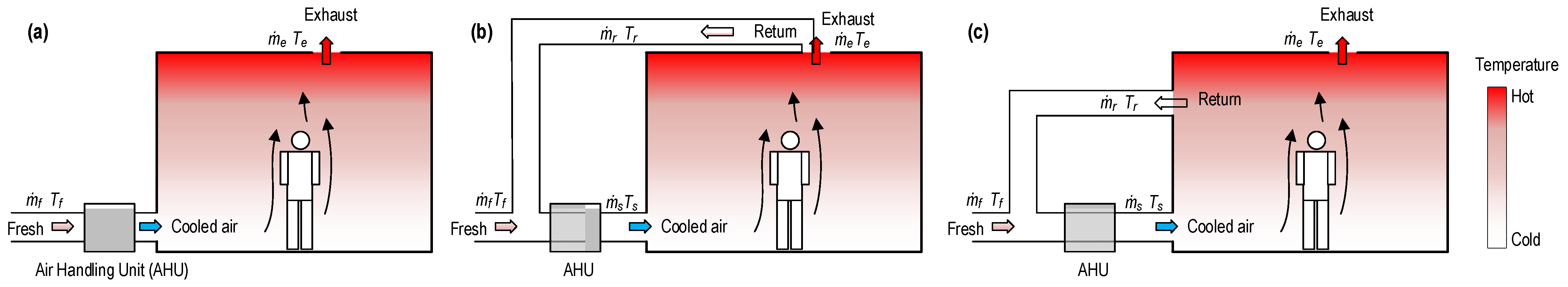
2.1. The Theoretical Analysis

For a STRAD system with exhaust/return-split layout (Figure 1c), the Q_coil is described in Equation (1) [8], and can be rearranged into Equation (2) [8]:

$$Q_{\mathrm{c}\mathrm{o}\mathrm{i}\mathrm{l}}=Q_{\mathrm{s}\mathrm{p}\mathrm{a}\mathrm{c}\mathrm{e}}-c_p{\dot{m}}_{\mathrm{f}}\left(T_{\mathrm{e}}-T_{\mathrm{f}}\right)$$

(1)

$$\frac{Q_{\mathrm{s}\mathrm{p}\mathrm{a}\mathrm{c}\mathrm{e}}}{c_p}={\dot{m}}_{\mathrm{r}}\left(T_{\mathrm{r}}-T_{\mathrm{s}}\right)+{\dot{m}}_{\mathrm{f}}\left(T_{\mathrm{e}}-T_{\mathrm{s}}\right)$$

(2)

where Q_coil is the cooling coil load; Q_space is the space cooling load consisting of external heat absorption, occupants, heat power facilities, and so on; c_p is the air heat capacity; and T_e, T_f, and T_f are the exhaust, fresh, and return air temperatures, respectively.

The T_r value is close to that of T_s when the return vent is near the supply diffuser, and it is close to T_e when the return vent is near the exhaust diffuser. We suppose an original assumption: T_r is a function of T_e and T_s, as shown in Equation (3).

$$T_{\mathrm{r}}=\left(1-\alpha \right)T_{\mathrm{e}}+\alpha T_{\mathrm{s}},\hspace{1em}\alpha \in \left[0,1\right]$$

(3)

where α is a fraction determined by the supply velocity. Equation (2) becomes Equation (4) by substituting Equation (3).

$$T_{\mathrm{e}}-T_{\mathrm{s}}=\frac{Q_{\mathrm{s}\mathrm{p}\mathrm{a}\mathrm{c}\mathrm{e}}}{c_p}\times \frac{1}{{\dot{m}}_{\mathrm{f}}+{\dot{m}}_{\mathrm{r}}\times \left(1-\alpha \right)}$$

(4)

When the return vent is located on the ceiling (Figure 1b), α = 0.

$$T_{\mathrm{e},0}-T_{\mathrm{s}}=\frac{Q_{\mathrm{s}\mathrm{p}\mathrm{a}\mathrm{c}\mathrm{e}}}{c_p}\times \frac{1}{{\dot{m}}_{\mathrm{f}}+{\dot{m}}_{\mathrm{r}}}$$

(5)

When the return vent is located on the floor, α = 1. As shown in Figure 1a, the return vents circulate supply air directly to the air handling unit, which has no effect of returning room air.

$$T_{\mathrm{e},1}-T_{\mathrm{s}}=\frac{Q_{\mathrm{s}\mathrm{p}\mathrm{a}\mathrm{c}\mathrm{e}}}{c_p}\times \frac{1}{{\dot{m}}_{\mathrm{f}}}$$

(6)

Equation (2) is converted to

$$\frac{Q_{\mathrm{s}\mathrm{p}\mathrm{a}\mathrm{c}\mathrm{e}}}{c_p}=\left\{{\dot{m}}_{\mathrm{f}}+{\dot{m}}_{\mathrm{r}}\left(1-\alpha \right)\right\}\left(T_{\mathrm{e}}-T_{\mathrm{s}}\right)$$

(7)

As a consequence, the theoretical maximum energy reduction due to the lowering of return vents is

$$Q_{\mathrm{c}\mathrm{o}\mathrm{i}\mathrm{l},0}-Q_{\mathrm{c}\mathrm{o}\mathrm{i}\mathrm{l},1}=c_p{\dot{m}}_{\mathrm{f}}\left(T_{\mathrm{e},1}-T_{\mathrm{e},0}\right)=c_p{\dot{m}}_{\mathrm{f}}\times \frac{Q_{\mathrm{s}\mathrm{p}\mathrm{a}\mathrm{c}\mathrm{e}}}{c_p}\times \frac{{\dot{m}}_{\mathrm{r}}}{{\dot{m}}_{\mathrm{f}}\times \left({\dot{m}}_{\mathrm{f}}+{\dot{m}}_{\mathrm{r}}\right)}=Q_{\mathrm{s}\mathrm{p}\mathrm{a}\mathrm{c}\mathrm{e}}\times \frac{{\dot{m}}_{\mathrm{r}}}{{\dot{m}}_{\mathrm{f}}+{\dot{m}}_{\mathrm{r}}}$$

(8)

The cooling coil load for the room without return vents is

$$Q_{\mathrm{c}\mathrm{o}\mathrm{i}\mathrm{l},1}=Q_{\mathrm{s}\mathrm{p}\mathrm{a}\mathrm{c}\mathrm{e}}-c_p{\dot{m}}_{\mathrm{f}}\left(T_{\mathrm{e},1}-T_{\mathrm{f}}\right)=Q_{\mathrm{s}\mathrm{p}\mathrm{a}\mathrm{c}\mathrm{e}}-c_p{\dot{m}}_{\mathrm{f}}\left(\frac{Q_{\mathrm{s}\mathrm{p}\mathrm{a}\mathrm{c}\mathrm{e}}}{c_p}\times \frac{1}{{\dot{m}}_{\mathrm{f}}}+T_{\mathrm{s}}-T_{\mathrm{f}}\right)=c_p{\dot{m}}_{\mathrm{f}}\left(T_{\mathrm{f}}-T_{\mathrm{s}}\right)$$

(9)

$$Q_{\mathrm{s}\mathrm{p}\mathrm{a}\mathrm{c}\mathrm{e}}=c_p{\dot{m}}_f\left(T_{e,1}-T_{\mathrm{s}}\right)$$

(10)

Considering that $T_{e,1}$ < $T_{\mathrm{f}}$, the air can be exhausted directly, Q_coil,1 > Q_space. Therefore, the energy saved is less than the minimum cooling coil load in all cases.

$$\frac{Q_{\mathrm{c}\mathrm{o}\mathrm{i}\mathrm{l},0}-Q_{\mathrm{c}\mathrm{o}\mathrm{i}\mathrm{l},1}}{Q_{\mathrm{c}\mathrm{o}\mathrm{i}\mathrm{l},1}}<1$$

(11)

The vertical temperature gradient is uniform when the temperature is well stratified [23]. The ratio of the increment in ΔT_0.1–1.1 to the minimum ΔT_0.1–1.1 is

$$\frac{{∆T}_{0.1-1.1,1}-{∆T}_{0.1-1.1,0}}{T_{\mathrm{e},0}-T_{\mathrm{s}}}=\frac{T_{\mathrm{e},1}-T_{\mathrm{e},0}}{T_{\mathrm{e},0}-T_{\mathrm{s}}}=\frac{\frac{1}{{\dot{m}}_{\mathrm{f}}}-\frac{1}{{\dot{m}}_{\mathrm{f}}+{\dot{m}}_{\mathrm{r}}}}{\frac{1}{{\dot{m}}_{\mathrm{f}}+{\dot{m}}_{\mathrm{r}}}}=\frac{{\dot{m}}_{\mathrm{r}}}{{\dot{m}}_{\mathrm{f}}}>1$$

(12)

We know that the variation in ΔT_0.1–1.1 is larger than that in Q_coil by comparing Equation (11) with Equation (12). Therefore, the benefit of energy savings is smaller than the cost of the temperature gradient, even if the weight of ΔT_0.1–1.1 is heavier than that of Q_coil according to the entropy method. Consequently, it can be concluded that a high H is more appropriate than a low H if the PMV and air quality are not considered. Notably, the theoretical analysis is independent of the ventilation type as long as the enclosure is ventilated with STRAD systems and well stratified.

Additionally, several studies have reported that lower vents lead to a shorter circuit of supply air to the return vent and leave the upper part of the space with older air, indicating worse air quality [4,16,22,24]. The PMV in the OZ is mainly determined by the supply temperature and supply airflow rate because the treated air is directly supplied to the OZ. For a lower vent, the air temperature in the OZ is closer to the supply temperature due to the short circuit airflow. Consequently, it is hard to conclude which system is better than another at creating an acceptable PMV when supply temperature and supply airflow rate are adjustable.

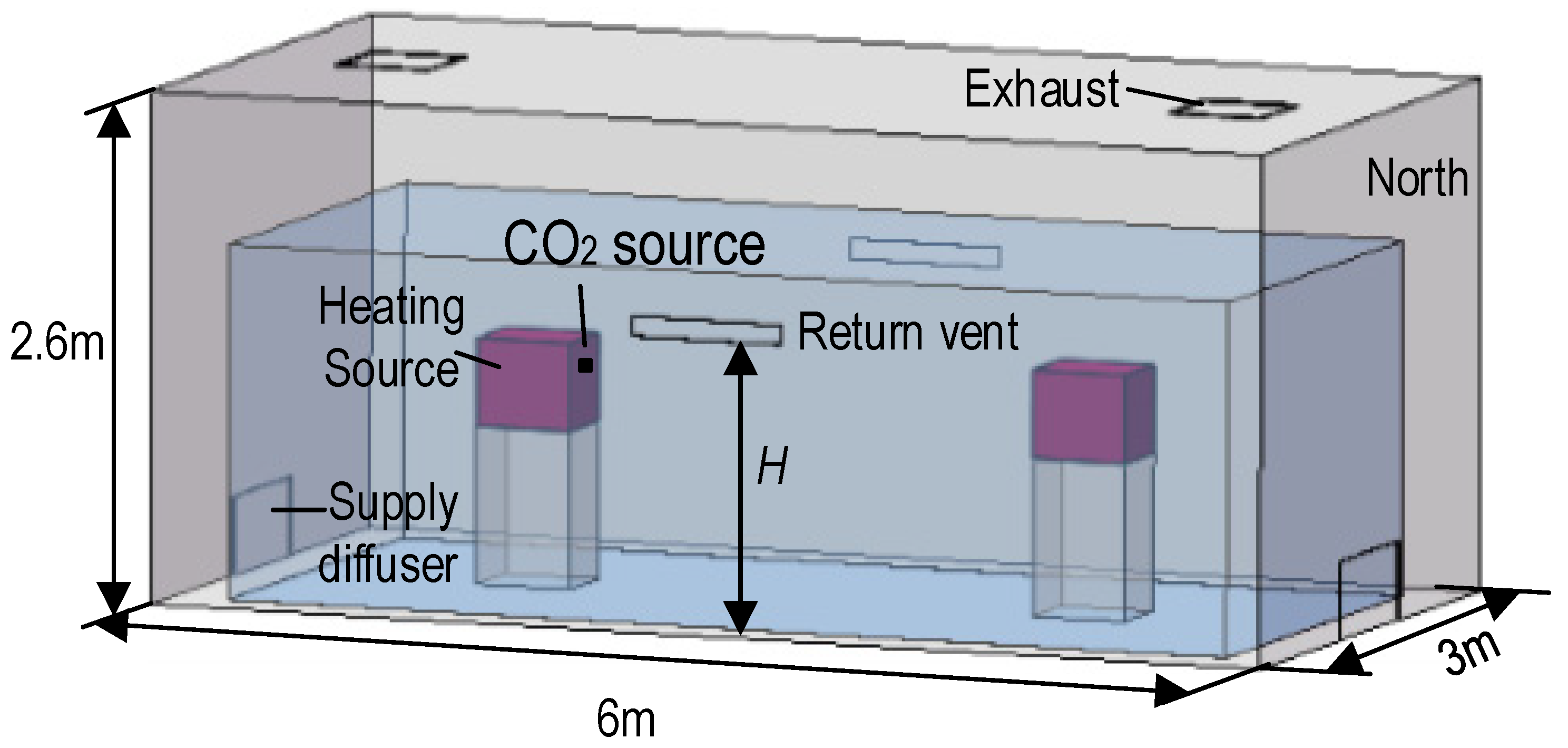
2.2. Study Object (Modeled Room)

The study object is a small office (consistent with the descriptions in ref. [25]) with dimensions of 3 m × 6 m × 2.6 m (as depicted in Figure 2). It is equipped with a pair of diffusers (both with an aperture of 0.8 m × 0.4 m) that channel low-temperature air into the office near the floor. A pair of ceiling exhausts (0.5 m × 0.5 m/each) expel a minor proportion of the heated air, while the majority is recirculated through a pair of return vents (with apertures of 0.8 × 0.1 m) situated on the northern and southern walls. The OZ is at a height of 1.8 m, 0.3 m (horizontal distance) from each office wall (marked in blue in Figure 2). The supply diffusers and exhausts are simulated in the form of individual apertures owing to the close resemblance between the velocity fields created by individual apertures and diffusers with slatted openings [4]. The variable subject to optimization is H. To save on computing costs, the simulated area only encompasses 25% of the total office space, considering the symmetry of this ventilated enclosure.

2.3. The Numerical Model

2.3.1. The Governing Equations

Air movement is modeled to be steady and incompressible in spaces with ventilation, with the buoyancy forces represented as momentum sources, and the transport of various field variables (e.g., energy or gas species) obeys the Navier–Stokes equations:

$$divU=0$$

(13)

$$\mathrm{d}\mathrm{i}\mathrm{v}\left(\rho U\Phi \right)=\mathrm{d}\mathrm{i}\mathrm{v}\left({\Gamma }_{\Phi }\mathrm{g}\mathrm{r}\mathrm{a}\mathrm{d}\Phi \right)+S_{\Phi }$$

(14)

where Φ is a transported variable (representing, e.g., energy or gas species) for which a diffusion coefficient Γ_Φ and a source term S_Φ are defined. The source term for thermal buoyancy obeys the incompressible ideal gas law in Equation (14), where Φ is the velocity component in the gravitational direction. The discrete ordinates method [26] is applied to model the radiative component of energy transfer. Turbulence is captured using the shear stress transport (SST) k-ω model [27]. ANSYS Fluent (19.2 version) was used to obtain a numerical solution for these equations.

2.3.2. Boundary Conditions

The boundary conditions are carefully set up according to ref. [4]. The floor and ceiling are assumed to be thermally adiabatic, and the temperature of the outdoor air is set at 30.8 °C, which is typical for the assumed location (Shanghai) in the summer months [28]. This study adapts the approach used in ref. [4], in which the through-wall solar heat flux is represented according to the convective heat transfer, leading to varying external temperatures based on the wall orientation. Accordingly, the overall equivalent heat transfer coefficient of the walls was 1.45 W/(m².K), and the outdoor temperatures were adjusted to 34.7 °C for the northern and southern walls and 39.7 °C for the western and eastern walls. Heat loading is considered to be equivalent to the heat power of the heating units, which is assumed to be 330 W each. CO₂ emissions are fixed at 0.31 L/min per sedentary occupant (i.e., 0.01 g/s at a height of 1.1 m), assuming the activity equals 1.2 metabolic equivalents [29]. The CO₂ supplied by the supply diffuser (0.091 m³/s per diffuser with a temperature of 18 °C or the value needed to achieve |PMV| < 0.5) is a mixture of returned air and fresh air [30] following Equation (15):

$$S_s=\frac{S_r{\dot{m}}_r+S_f{\dot{m}}_f}{{\dot{m}}_s}$$

(15)

where S_s and S_r represent the CO₂ mass fraction at the supply diffuser and the return vent, respectively, while S_f is the corresponding value for fresh air.

2.4. Ventilation Performance Indices

A detailed discussion of the performance indices is given in ref. [22]. Q_coil is taken as the measure of energy consumption, as follows:

$$Q_{\mathrm{c}\mathrm{o}\mathrm{i}\mathrm{l}}=Q_{\mathrm{s}\mathrm{p}\mathrm{a}\mathrm{c}\mathrm{e}}-c_p{\dot{m}}_{\mathrm{f}}\left(T_{\mathrm{e}}-T_{\mathrm{f}}\right)$$

(16)

where Q_space is the space cooling load with contributions from external heat absorption, occupants’ metabolism heat, and facilities’ heat powers, among other components; c_p represents the air heat capacity; and T_f (T_e) are the temperatures of fresh (exhaust) air. The IAQ is calculated according to the OZ-averaged MAA and OZ-averaged concentration of CO₂. Thermal comfort is quantified using Fanger’s PMV-PPD model [13,31], DR [13], and ΔT_0.1–1.1 (i.e., the difference in temperature when z = 0.1 m and z = 1.1 m for sedentary occupants).

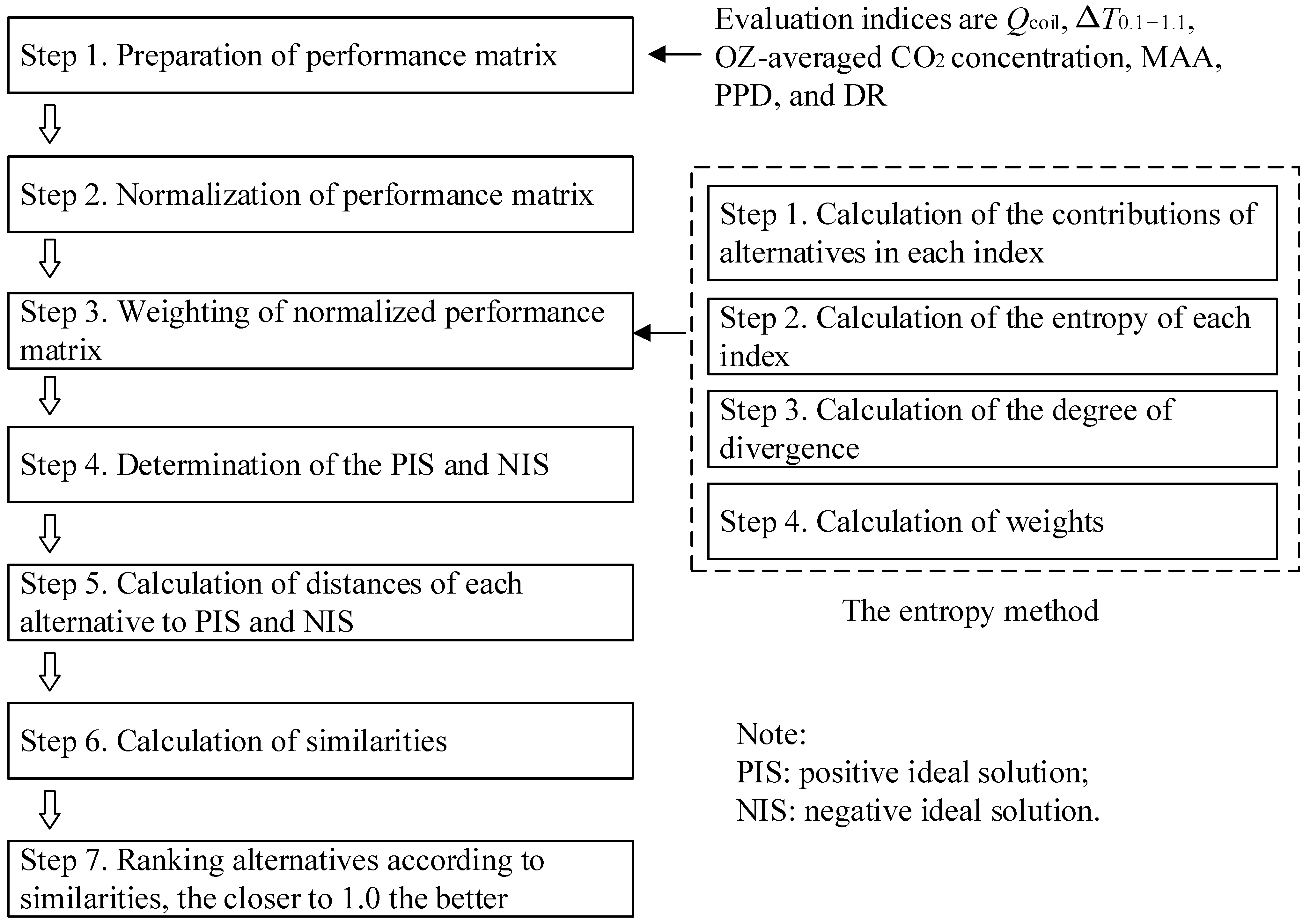
2.5. Optimization Algorithm: Entropy-Based TOPSIS

The multi-criteria optimization algorithm might be appropriate to optimize the H for STRAD systems. As H is a single factor influencing several evaluation criteria, it could be applied to evaluate the difference within an index when the minimum standards are met (e.g., the difference when ΔT_0.1–1.1 is below 3 °C). Among the various types of multi-criteria optimization algorithms, TOPSIS has been widely used in the context of ventilation optimization. Due to the lack of weights, this study selects the entropy method to weigh each criterion.

The entropy-based TOPSIS (E-TOPSIS) consists of two parts: a ranking algorithm (TOPSIS) and weight calculation (the entropy method). The entropy method weighs each criterion according to the information [32] contained in the criterion (i.e., the diversity of the criterion caused by various alternatives). In the TOPSIS method, similarity values are calculated according to the distance of each alternative with respect to positive and negative ideal solutions, and then the alternatives are ranked based on their similarity values. The detailed procedure of the E-TOPSIS [2,22,33,34] method is shown in Figure 3.

3. Validation of Numerical Model and Grid Independence Testing

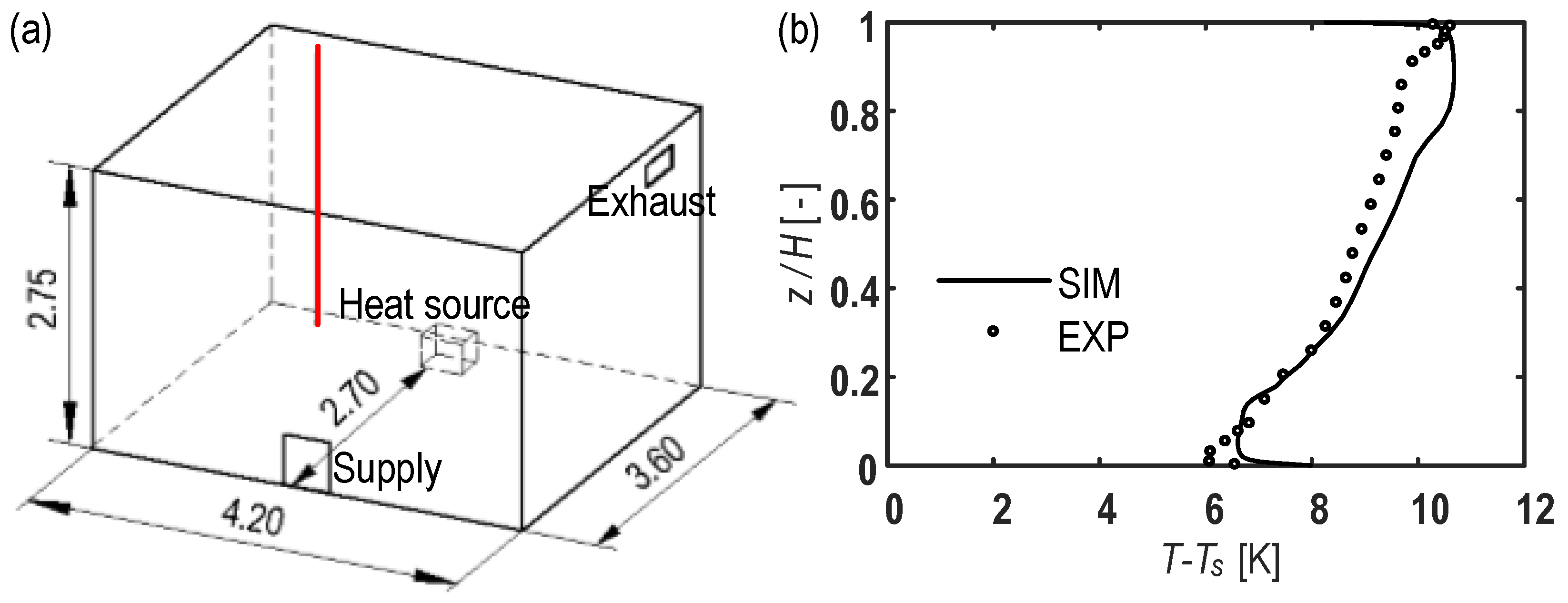
3.1. Numerical Model Validation

We validated the CFD model before it was used to simulate airflows. The validation tests were conducted in a simulated displacement-ventilated enclosure (Figure 4a), in which the measured temperature was the same as that reported in ref. [35]. The velocity and temperature of the treated air supply were 0.053 m/s and 16.0 °C. The heat flux from the heat source surface was 8333.3 W/m². The ceiling and floor temperatures were 24.2 °C and 24.0 °C, respectively. The boundary condition of the vertical walls’ temperature is provided as the average value of the measured temperatures of the walls at five different heights, according to the testing data provided in ref. [35] (

Table 1. Temperature of vertical walls at five different heights [35,36].

Wall Height [m]	Temperature [°C]
0.08	22.4
0.73	23.4
1.39	24.0
2.04	24.5
2.68	24.4

). Figure 4b shows that the simulated thermal profile matches the experimentally measured data, thus validating the numerical model.

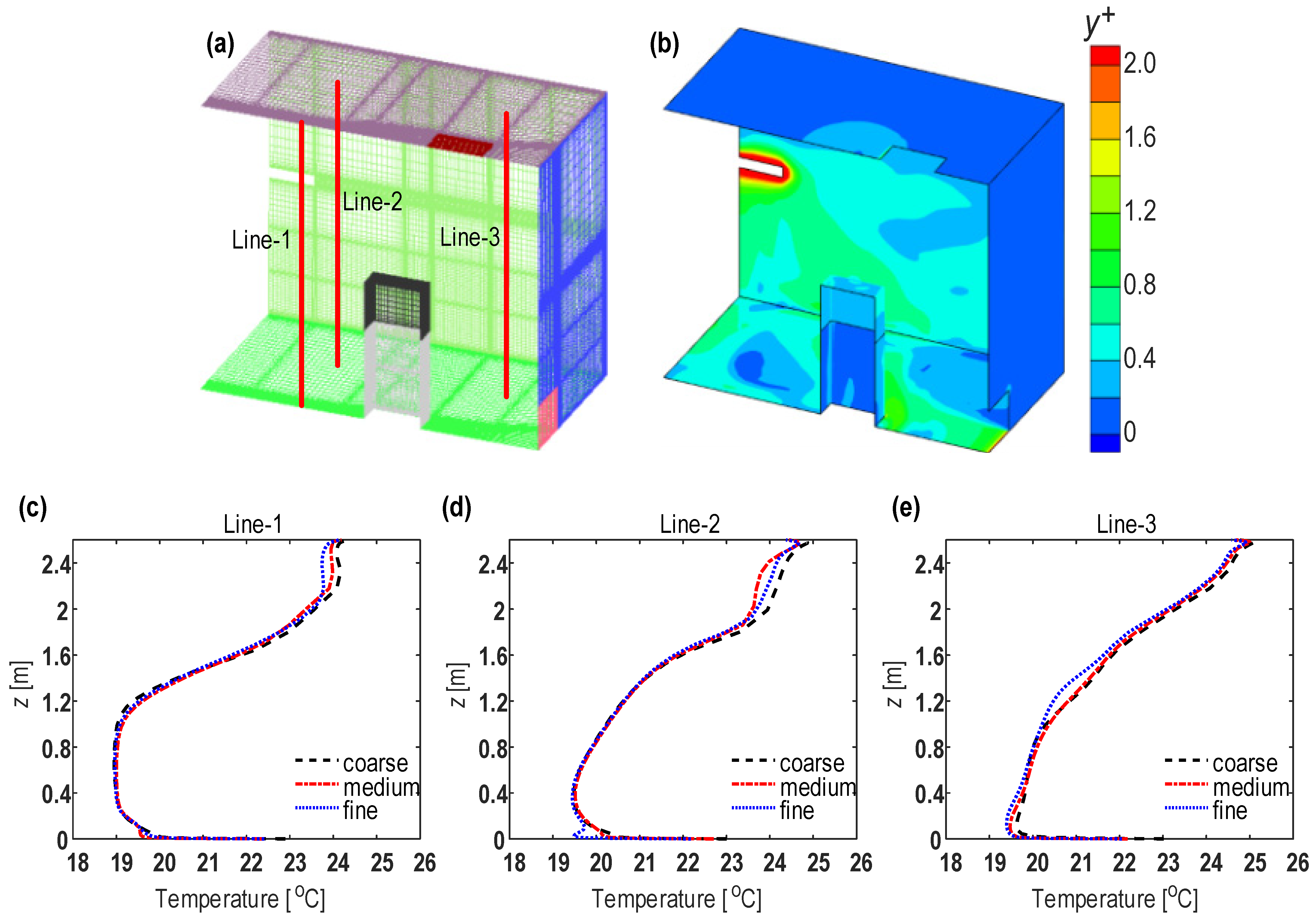
3.2. Grid Independence Testing

A grid independence test was conducted with an H value of 1.3 m to ensure that the simulation outcomes were not biased by the grid resolution. Three resolutions were compared: a low-resolution grid (267,600 grid cells), a moderate-resolution grid (608,175 grid cells), and a high-resolution grid (1,145,263 grid cells). These grids were built using ANSYS ICEM (Figure 5a). The first cell layer lies within the viscous sublayer (y⁺ < 5), as Figure 5b shows, satisfying the requirements of the SST k-ω model [27]. The simulated temperature profiles based on all three grids are similar (Figure 5c–e). The calculation of the grid convergence index (GCI) [37] reveals the dependence of the simulation outcomes on the grid resolution. All GCI values (

Table 2. GCI values along Lines 1–3.

Line	1	2	3
GCIc,m * [%]	0.1	0.7	0.2
GCIm,f [%]	0.1	0.2	0.2

* The labels c, m, and f in subscript denote, respectively, low-resolution (coarse), moderate-resolution (medium), and high-resolution (fine) grids.

) are under 5%, meaning the three grids are all acceptable. The moderate-resolution grid was selected, as when using the low-resolution grid, the scaled residual of the iterated continuity equation exceeded 1 × 10⁻³.

4. Results and Discussion

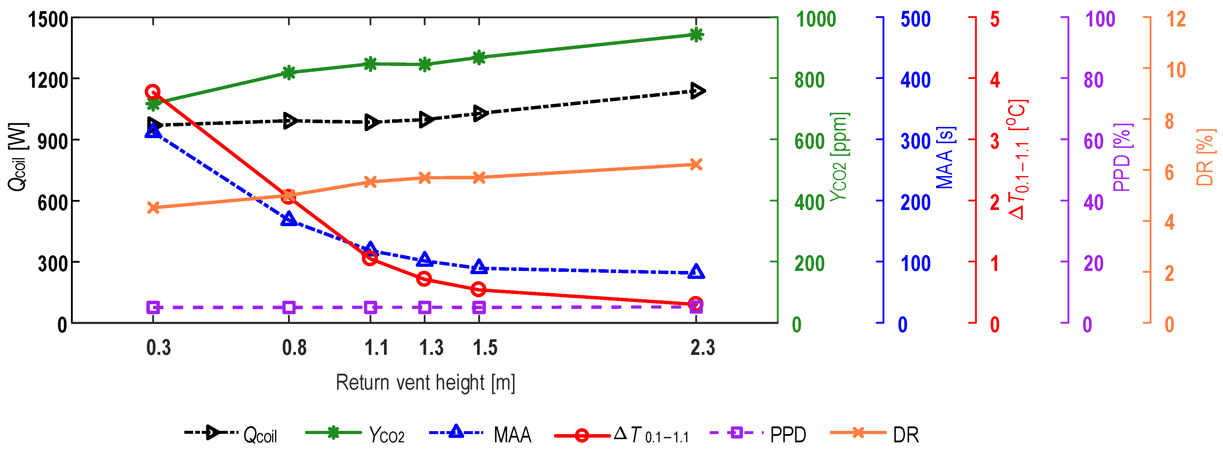
4.1. Optimizing H with Fixed T_s

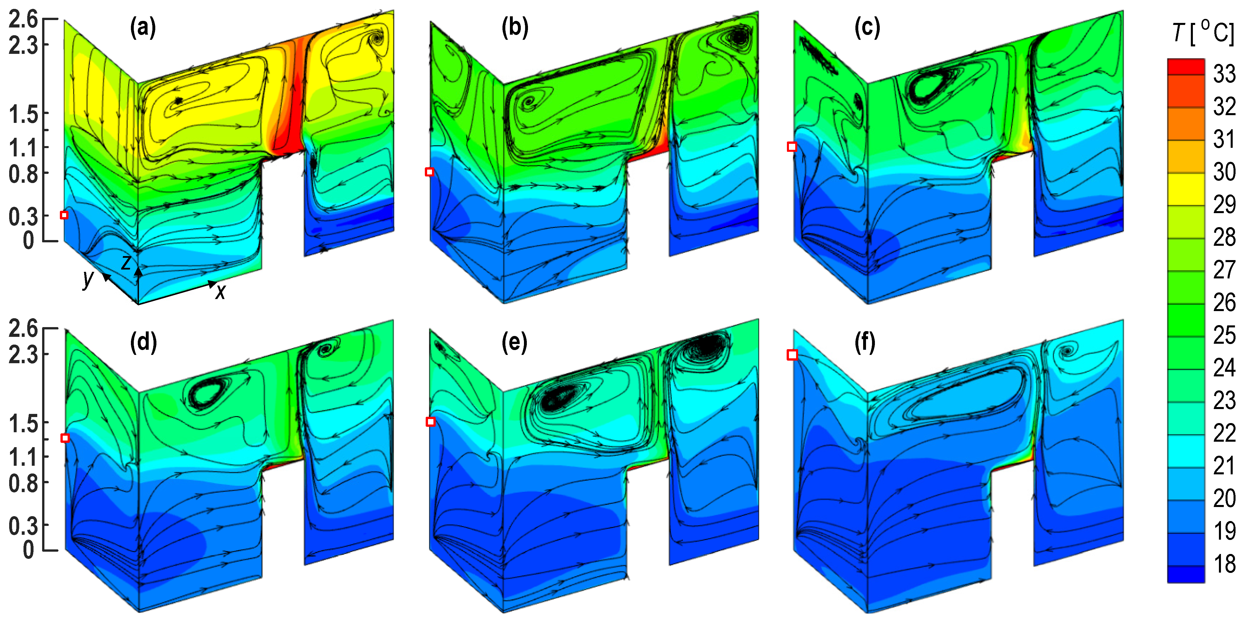
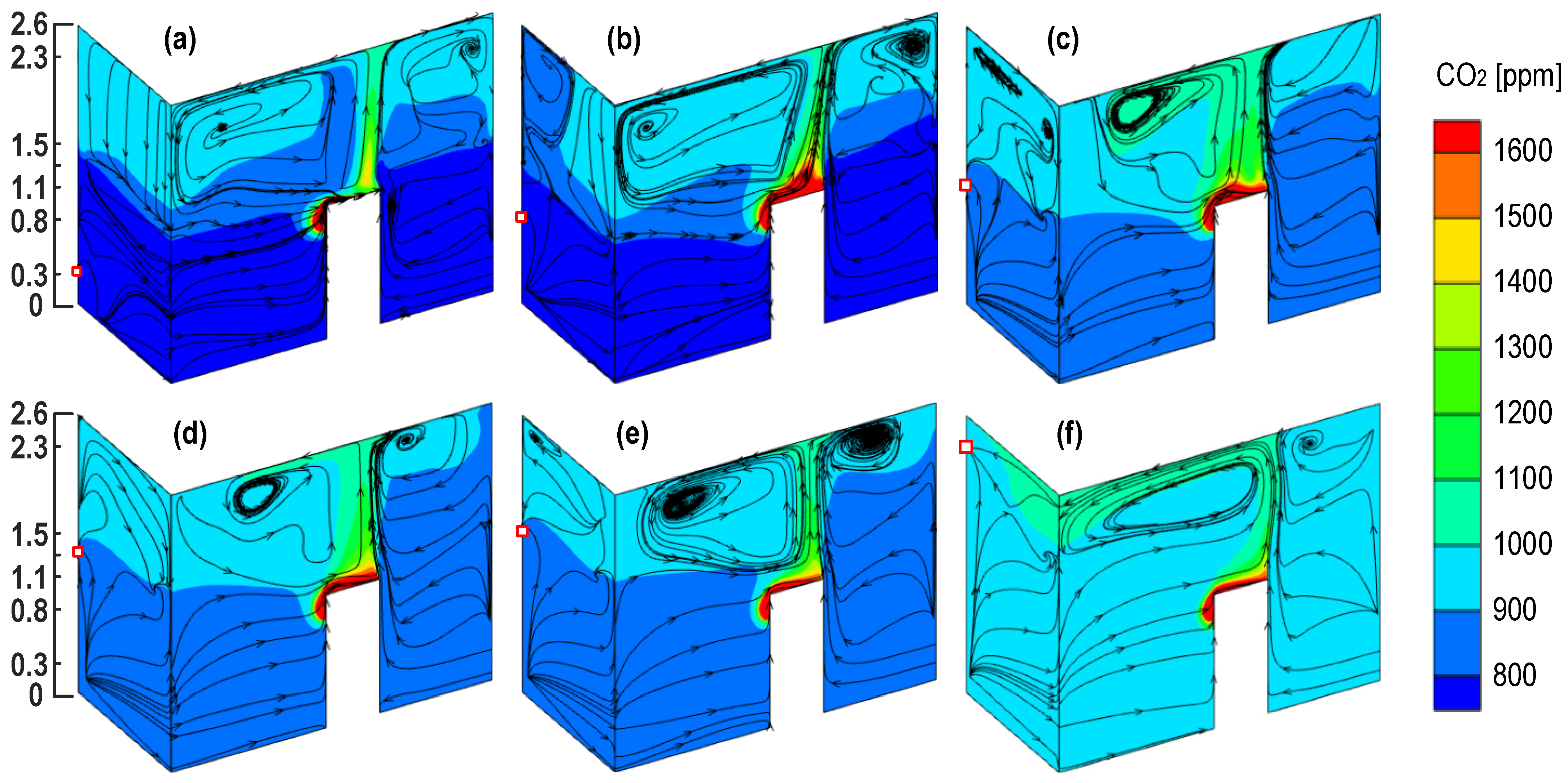
4.1.1. Temperature Fields

Figure 6 presents the thermal contours. Consistent with ref. [38], the DV system supplies cold air into the OZ, leading to thermal stratification in the enclosure. The heat source plume flows upward and impinges on the ceiling, carrying warm air upward. When the vents are at a lower H, more heat accumulates in the upper portion of the office space because the vents remove (cooler) air from the lower portion. As a consequence, the room temperature drops as H increases, which is concordant with extant research [4,8,9,10,16,17,22] on IJV and UFAD systems.

4.1.2. Thermal Comfort Comparison

Figure 7 shows the thermal comfort performances under various H values. The PMV and ΔT_0.1–1.1 drop as the H increases, which is consistent with the temperature distributions under various H values (Section 4.1.1). In most of these cases (excluding only H = 0.3 m), the room is overcooled, i.e., the PMV < −0.5 [12]. In contrast, ΔT_0.1–1.1 is too large when H equals 0.3 m (>3 °C). In other words, when the requirement for the PMV is met, the requirement for ΔT_0.1–1.1 is not met, so none of these cases are thermally comfortable.

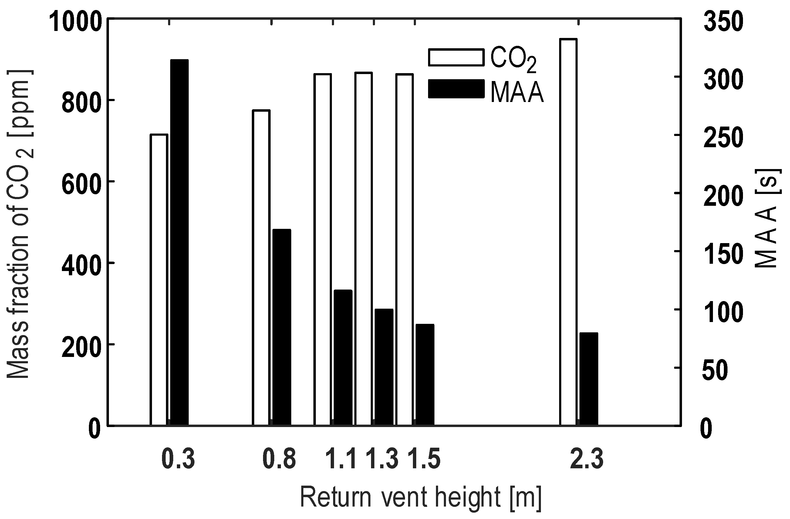
4.1.3. Comparison of IAQ Performance

The CO₂ distribution is stratified (Figure 8), akin to the stratification of temperature. This is because the thermal plume entrains CO₂, as reported in the literature [6,39]. The CO₂ concentration increases as H increases, which is consistent with ref. [40] but differs from previously reported observations for impinging jet ventilation [16]. These inconsistencies can be explained by the fact that the body plume was terminated at the mid-level in ref. [16], meaning that the mid-level return vent was closer to the plume-entrained contaminants, while the plume impinges the ceiling in this study. On the other hand, the higher vent creates a more uniform CO₂ distribution, indicating that a lower CO₂ concentration is removed from the exhaust, which is similar to the variation in temperature. The OZ-averaged CO₂ concentration shows a quantitatively increasing trend, and the age of the air in the OZ reduces as H increases (Figure 9), which is consistent with refs. [2,4,10,16,17,22,24].

4.1.4. The Optimal H

Figure 10 summarizes the ventilation performance under various H values. As H increases, the Q_coil, CO₂ concentration, PPD, and DR values increase, while ΔT_0.1–1.1 and MAA decrease. The cost of thermal comfort evaluated by the PPD is caused by overcooling, as demonstrated in Section 4.1.2 and Section 4.1.3. The cost of ΔT_0.1–1.1 is larger than the benefit of Q_coil, which is consistent with the theoretical analysis in Section 2.5. For all of these indices, smaller values indicate better performance. Hence, a multi-objective optimization algorithm is appropriate to determine the best among these cases. The TOPSIS-calculated similarities are shown in

Table 3. Similarity/ranking for T_s = 18 °C.

H [m]	0.3	0.8	1.1	1.3	1.5	2.3
Similarity	0.1758	0.4806	0.7499	0.8065	0.8221	0.8242
Ranking	6	5	4	3	2	1

. The optimal H is 2.3 m. However, the similarities of cases with H = 1.5 m and 2.3 m are close to each other, indicating an optimal range of 1.5–2.3 m. The suitability of a mid-level H of 1.5 m is consistent with the suggestion of similar levels in refs. [16,17,22], in which H was optimized under fixed supply parameters. However, the near-ceiling height (H = 2.3 m) was not suggested in previous studies under the given supply parameters. This discrepancy might be due to the differences in the trends of CO₂ concentration. The CO₂ concentration was found to decrease with an increasing H value in previous research, while it increased with an increasing H in this study.

4.2. Optimization Subject to Thermoneutrality Requirement

4.2.1. Achieving Thermoneutrality via Adjusting T_s

T_s was tuned to achieve thermoneutrality (i.e., |PMV| is less than 0.5), and it was found that T_s must be adjusted to 20.0, 22.0, 23.0, 23.5, 24.0, and 24.0 °C for the respective H values of 0.3, 0.8, 1.1, 1.3, 1.5, and 2.3 m (Figure 11). The final PMVs under the various H values are all close to zero in the standing OZ, thus meeting the thermoneutrality requirement.

4.2.2. Optimal H Given the Requirement That |PMV| Is Less Than 0.5

Figure 12 summarizes the ventilation performances under the thermoneutral condition for various H values. The PPD is low in all cases, which is the main difference between the condition involving fixed supply parameters (Figure 10) and the thermoneutral condition. The similarities and corresponding rankings are reported in

Table 4. Similarity values and rankings for H under the OZ thermoneutrality condition (|PMV| < 0.5).

H [m]	0.3	0.8	1.1	1.3	1.5	2.3
Similarity	0.0028	0.5055	0.7889	0.8837	0.9328	0.9972
Ranking	6	5	4	3	2	1

. The highest similarity is 0.9972, which is very close to 1.0, indicating that the benefits in terms of the MAA and ΔT_0.1–1.1 are so large that the costs in terms of the Q_coil, CO₂ concentration, and DR values can be ignored.

The optimal performance assuming fixed supply parameters and thermoneutrality is summarized in

Table 5. Evaluation metrics under optimal cases given |PMV| < 0.5 and T_s = 18 °C.

Optimal Cases	Average MAA [s]	Qcoil [W]	Average CO2 [ppm]	ΔT0.1–1.1 [°C]	DR [%]	PPD [%]
Ts = 18 °C, H = 1.5 m	86.7	1264.5	863.1	0.54	9.5	72.7
Ts = 18 °C, H = 2.3 m	79.5	1393.7	949.5	0.30	10.3	78.8
|PMV| < 0.5, H = 2.3 m	81.4	1139.9	943.2	0.30	6.2	5.2

. The optimal H spans 1.5–2.3 m under the fixed supply parameter case (i.e., between the mid-level and near-ceiling level) and is 2.3 m under the thermoneutral condition. When the H value is 2.3 m, the main differences in performance between the two conditions are related to energy consumption and thermal comfort. Compared with the condition of fixed supply parameters, the PPD drops from 78.8% to 5.2%, and the DR drops from 10.3% to 6.2%. The Q_coil value drops by 18.2% under the thermoneutral condition (i.e., from 1393.7 W to 1139.9 W). Compared with the case of H = 1.5 m and T_s = 18 °C, the performances are improved for each evaluation metric except for CO₂ removal under the thermoneutral condition. Notably, H is difficult to change in practice after the construction period. Therefore, the results of this study suggest that optimization under thermoneutral conditions is preferable.

4.3. Limitations

Despite performing theoretical and numerical investigations of the impacts of H on the performances of stratified air distribution systems, this study still has several limitations. First, the theoretical analysis quantitatively compared the Q_coil with the vertical temperature difference and discusses the age of the air, while the PMV was not compared. Second, the comparison in the theoretical analysis indicated that the weights of the evaluation indices are equal. In reality, the users may prioritize saving energy, improving air quality, or maintaining thermal comfort. Third, heat sources were simplified into heating boxes, which induces a plume that is too strong impinging on the ceiling, while the body plume may be not so strong though it still entrains breathing CO₂ [41]. This deviation may enhance CO₂ transfer. Finally, the only boundary condition of an outdoor parameter in our study was the temperature and we did not validate the influence of the location’s climatic parameters. Further research can focus on a theoretical analysis of the age of air and CO₂ transfer in an enclosure ventilated with a general STRAD system and validate the theoretical model with different climate parameters.

5. Conclusions

This research examined the effect of the H on a STRAD system’s performance, taking a DV system as an illustrative case. The evaluation metrics comprised a set of widely used factors, namely energy consumption (i.e., Q_coil), the IAQ (i.e., MAA, CO₂ concentration), and thermal comfort (i.e., PMV, PPD, ΔT_0.1–1.1, and DR). Optimization was performed using the TOPSIS algorithm with weights calculated via the entropy method. The key findings and their implications are as follows:

(a)

A theoretical analysis demonstrated that the amount of energy saved when using a lower vent is smaller than the cost of the vertical temperature gradient for all STRAD systems.

(b)

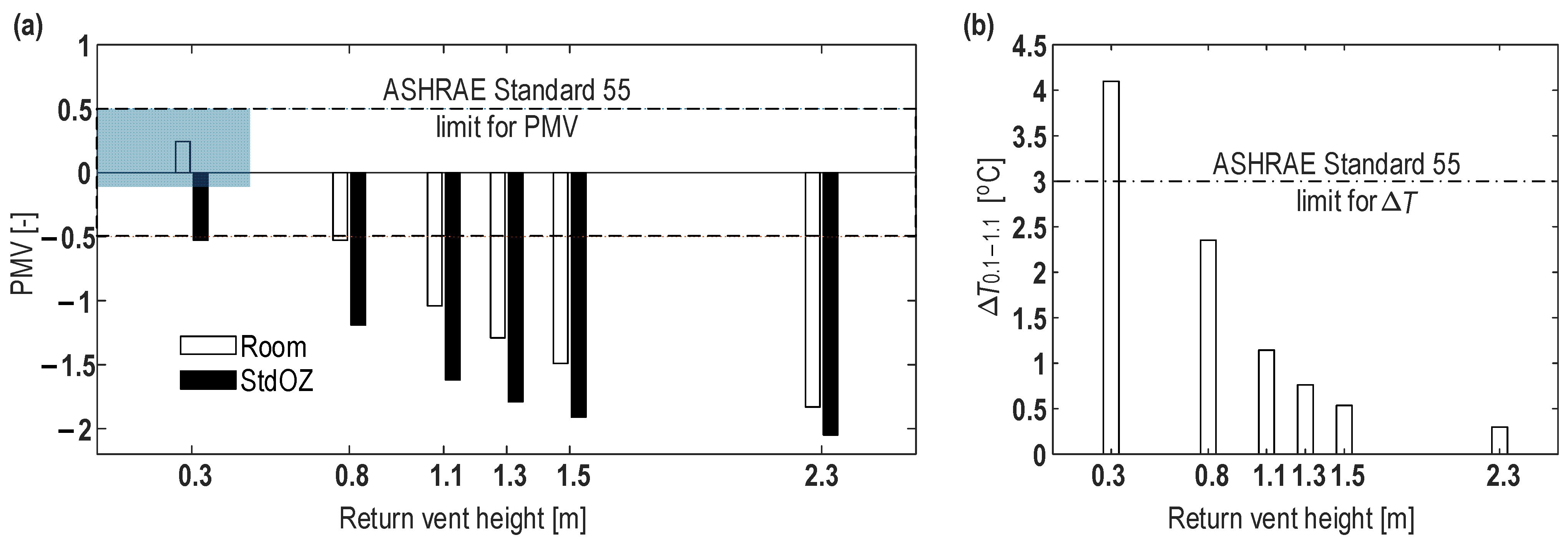
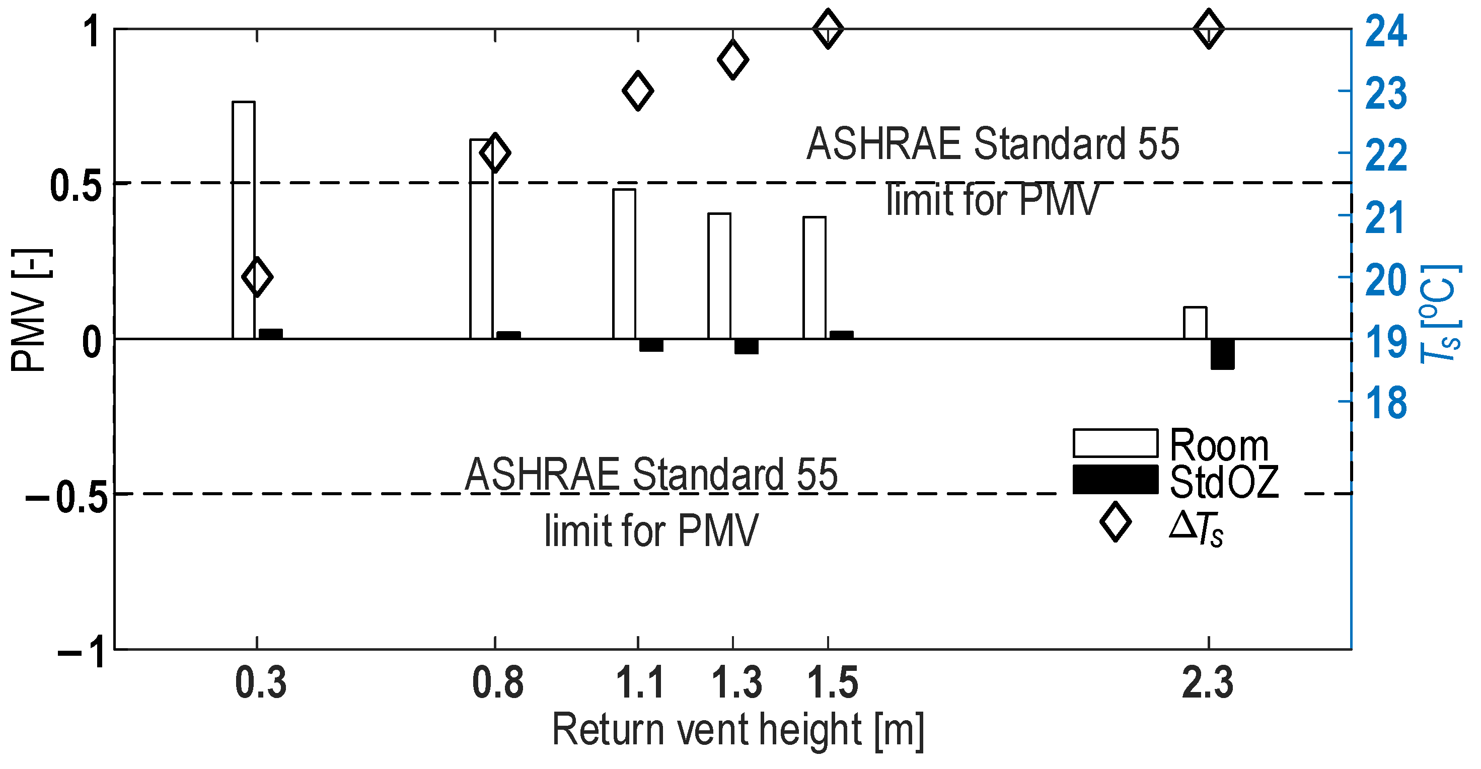
When T_s is 18 °C, the PMV is under −0.5 in most cases except when the H is 0.3 m; that is, the studied enclosure (an office room) is overcooled. The TOPSIS method suggested 1.5–2.3 m as the optimal range.

(c)

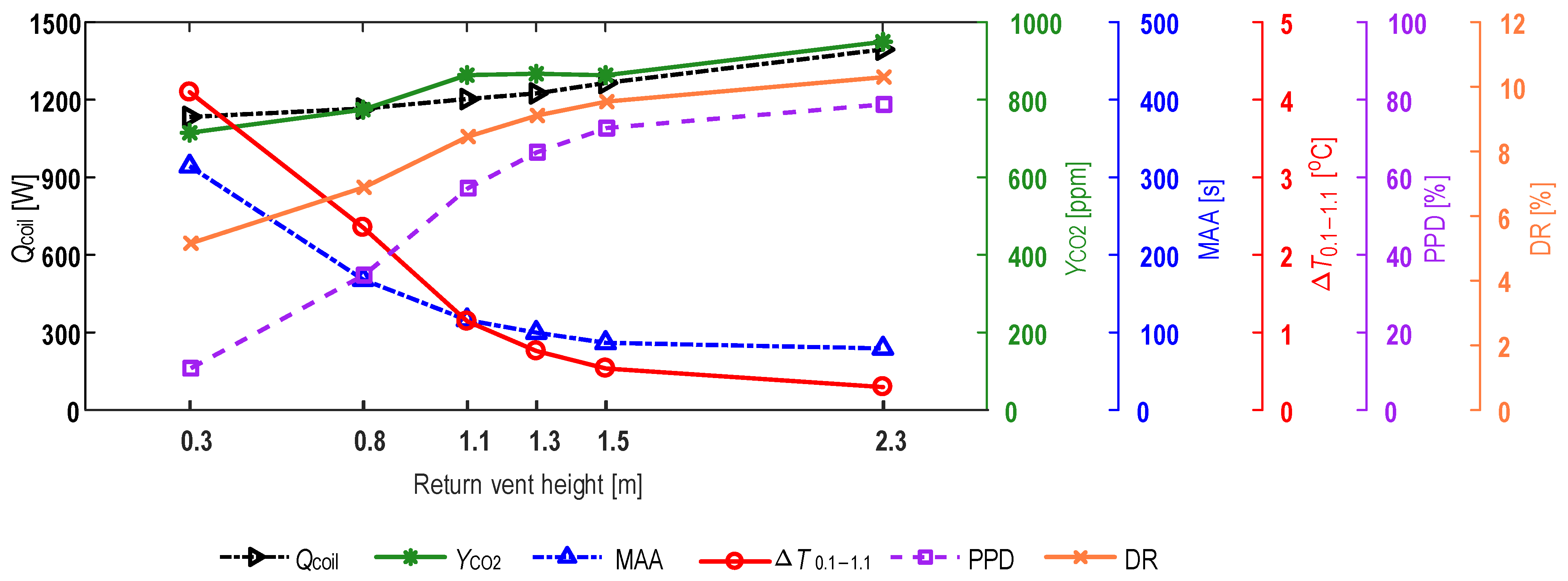
When T_s is adjusted to achieve a thermal neutral environment, the suggested optimal H is 2.3 m. In this case, the benefits on the MAA and ΔT_0.1–1.1 are so large that the costs in terms of the Q_coil value, concentration of CO₂, and DR can be ignored.

(d)

The optimal case under thermoneutral conditions is preferable with respect to the IAQ, reduced energy consumption, and thermal comfort, compared with those of the optimal H ranging from 1.5 m to 2.3 m at a T_s of 18 °C with a fixed supply temperature. A near-ceiling H is suggested.

In this study, we explored the optimization of H in STRAD systems, focusing specifically on DV systems. Our findings suggest that an H value of 2.3 m, when coupled with a thermoneutral condition, strikes an optimal balance between energy efficiency, IAQ, and thermal comfort. The application of the TOPSIS methodology, underpinned by an entropy-based weighting approach, facilitated a nuanced optimization that prioritizes thermal neutrality. Such optimization is particularly beneficial for environments seeking to reduce energy consumption without compromising occupant comfort or air quality.

The beneficiaries of our research include architects, heating ventilation and air-conditioning (HVAC) engineers, and building designers who aim to implement STRAD systems in their projects. By adhering to our recommended parameters, these stakeholders can enhance the sustainability and occupant satisfaction of their buildings. Furthermore, our study contributes to the broader discourse on sustainable building practices by demonstrating the efficacy of H optimization in reducing energy consumption while maintaining a comfortable and healthy indoor environment.

References

1. Wei, G.; Chen, B.; Lai, D.; Chen, Q. An improved displacement ventilation system for a machining plant. Atmos. Environ. 2020, 228, 117419. [Google Scholar] [CrossRef]
2. Qin, C.; Zhou, W.-R.; Fang, H.-Q.; Lu, W.-Z.; Lee, E.W. Optimization of return vent height for stratified air distribution system with impinging jet supply satisfying threshold of |PMV| < 0.5. J. Clean. Prod. 2022, 359, 132033. [Google Scholar]
3. Hu, J.; Kang, Y.; Yu, J.; Zhong, K. Numerical study on thermal stratification for impinging jet ventilation system in office buildings. Build. Environ. 2021, 196, 107798. [Google Scholar] [CrossRef]
4. Fan, Y.; Li, X.; Yan, Y.; Tu, J. Overall performance evaluation of underfloor air distribution system with different heights of return vents. Energy Build. 2017, 147, 176–187. [Google Scholar] [CrossRef]
5. Johnson, R.; Burroughs, C. Reducing Airborne Particulates Using Displacement Ventilation. ASHRAE J. 2022, 64, 38–48. [Google Scholar]
6. Yang, R.; Ng, C.S.; Chong, K.L.; Verzicco, R.; Lohse, D. Do increased flow rates in displacement ventilation always lead to better results? J. Fluid Mech. 2022, 932, A3. [Google Scholar] [CrossRef]
7. Liu, S.; Koupriyanov, M.; Paskaruk, D.; Fediuk, G.; Chen, Q. Investigation of airborne particle exposure in an office with mixing and displacement ventilation. Sustain. Cities Soc. 2022, 79, 103718. [Google Scholar] [CrossRef] [PubMed]
8. Cheng, Y.; Yang, J.; Du, Z.; Peng, J. Investigations on the energy efficiency of stratified air distribution systems with different diffuser layouts. Sustainability 2016, 8, 732. [Google Scholar] [CrossRef]
9. Cheng, Y.; Niu, J.; Gao, N. Stratified air distribution systems in a large lecture theatre: A numerical method to optimize thermal comfort and maximize energy saving. Energy Build. 2012, 55, 515–525. [Google Scholar] [CrossRef]
10. Heidarinejad, G.; Fathollahzadeh, M.H.; Pasdarshahri, H. Effects of return air vent height on energy consumption, thermal comfort conditions and indoor air quality in an under floor air distribution system. Energy Build. 2015, 97, 155–161. [Google Scholar] [CrossRef]
11. Fathollahzadeh, M.H.; Heidarinejad, G.; Pasdarshahri, H. Prediction of thermal comfort, IAQ, and energy consumption in a dense occupancy environment with the under floor air distribution system. Build. Environ. 2015, 90, 96–104. [Google Scholar] [CrossRef]
12. ASHRAE55; ANSI/ASHRAE Standard 55–2023. Thermal Environmental Conditions for Human Occupancy: Atlanta, GA, USA, 2023.
13. ISO7730; Ergonomics of the Thermal Environment, Analytical Determination and Interpretation of Thermal Comfort Using Calculation of the PMV and PPD Indices and Local Thermal Comfort Criteria. International Organization for Standardization: Geneva, Switzerland, 2005.
14. Shokrollahi, S.; Hadavi, M.; Heidarinejad, G.; Pasdarshahri, H. Multi-objective optimization of underfloor air distribution (UFAD) systems performance in a densely occupied environment: A combination of numerical simulation and Taguchi algorithm. J. Build. Eng. 2020, 32, 101495. [Google Scholar] [CrossRef]
15. Heidarinejad, G.; Shokrollahi, S.; Pasdarshahri, H. An investigation of thermal comfort, IAQ, and energy saving in UFAD systems using a combination of Taguchi optimization algorithm and CFD. Adv. Build. Energy Res. 2021, 15, 799–817. [Google Scholar] [CrossRef]
16. Ye, X.; Kang, Y.; Yan, Z.; Chen, B.; Zhong, K. Optimization study of return vent height for an impinging jet ventilation system with exhaust/return-split configuration by TOPSIS method. Build. Environ. 2020, 177, 106858. [Google Scholar] [CrossRef]
17. Qin, C.; Fang, H.-Q.; Wu, S.-H.; Lu, W.-Z. Establishing multi-criteria optimization of return vent height for underfloor air distribution system. J. Build. Eng. 2022, 57, 104800. [Google Scholar] [CrossRef]
18. Zhang, S.; Ai, Z.; Lin, Z. Novel demand-controlled optimization of constant-air-volume mechanical ventilation for indoor air quality, durability and energy saving. Appl. Energy 2021, 293, 116954. [Google Scholar] [CrossRef]
19. Anand, P.; Sekhar, C.; Cheong, D.; Santamouris, M.; Kondepudi, S. Occupancy-based zone-level VAV system control implications on thermal comfort, ventilation, indoor air quality and building energy efficiency. Energy Build. 2019, 204, 109473. [Google Scholar] [CrossRef]
20. Fisk, W.J.; De Almeida, A.T. Sensor-based demand-controlled ventilation: A review. Energy Build. 1998, 29, 35–45. [Google Scholar] [CrossRef]
21. Alaidroos, A.; Almaimani, A.; Krarti, M.; Dahlan, A.; Maddah, R. Evaluation of the performance of demand control ventilation system for school buildings located in the hot climate of Saudi Arabia. Build. Simul. 2022, 15, 1067–1082. [Google Scholar] [CrossRef]
22. Qin, C.; Wu, S.-H.; Fang, H.-Q.; Lu, W.-Z. The impacts of evaluation indices and normalization methods on E-TOPSIS optimization of return vent height for an impinging jet ventilation system. Build. Simul. 2022, 15, 2081–2095. [Google Scholar] [CrossRef]
23. Lee, J.H.-W.; Chu, V.H. Turbulent Jets and Plumes: A Lagrangian Approach; Springer Science & Business Media: New York, NY, USA, 2012. [Google Scholar]
24. Fan, Y.; Li, X.; Zheng, M.; Weng, R.; Tu, J. Numerical study on effects of air return height on performance of an underfloor air distribution system for heating and cooling. Energies 2020, 13, 1070. [Google Scholar] [CrossRef]
25. Wan, M.; Chao, C. Numerical and experimental study of velocity and temperature characteristics in a ventilated enclosure with underfloor ventilation systems. Indoor Air 2005, 15, 342–355. [Google Scholar] [CrossRef]
26. Kong, B.; Vigil, R.D. Simulation of photosynthetically active radiation distribution in algal photobioreactors using a multidimensional spectral radiation model. Bioresour. Technol. 2014, 158, 141–148. [Google Scholar] [CrossRef]
27. ANSYS Inc. ANSYS Fluent Theory Guide; ANSYS Inc.: Athens, Greece, 2015. [Google Scholar]
28. GB50736; China Architecture and Building Press, the People’s Republic of China National Standard GB 50736-2012, Design Code for Heating, Ventilation and Air Conditioning of Civil Buildings. China Academy of Building Research: Beijing, China, 2012. (In Chinese)
29. ASHRAE62.1; ANSI/ASHRAE Standard 62.1-2010. Ventilation for Acceptable Indoor Air Quality: Atlanta, GA, USA, 2010.
30. Qin, C.; Zhang, S.-Z.; Li, Z.-T.; Wen, C.-Y.; Lu, W.-Z. Transmission mitigation of COVID-19: Exhaled contaminants removal and energy saving in densely occupied space by impinging jet ventilation. Build. Environ. 2023, 232, 110066. [Google Scholar] [CrossRef]
31. Fanger, P. Thermal environment—Human requirements. Environmentalist 1986, 6, 275–278. [Google Scholar] [CrossRef]
32. Shannon, C.E. A mathematical theory of communication. Bell Syst. Tech. J. 1948, 27, 379–423. [Google Scholar] [CrossRef]
33. Park, J.H.; Park, I.Y.; Kwun, Y.C.; Tan, X. Extension of the TOPSIS method for decision making problems under interval-valued intuitionistic fuzzy environment. Appl. Math. Model. 2011, 35, 2544–2556. [Google Scholar] [CrossRef]
34. Mao, N.; Song, M.; Deng, S. Application of TOPSIS method in evaluating the effects of supply vane angle of a task/ambient air conditioning system on energy utilization and thermal comfort. Appl. Energy 2016, 180, 536–545. [Google Scholar] [CrossRef]
35. Li, Y.; Sandberg, M.; Fuchs, L. Effects of thermal radiation on airflow with displacement ventilation: An experimental investigation. Energy Build. 1993, 19, 263–274. [Google Scholar] [CrossRef]
36. Gilani, S.; Montazeri, H.; Blocken, B. CFD simulation of stratified indoor environment in displacement ventilation: Validation and sensitivity analysis. Build. Environ. 2016, 95, 299–313. [Google Scholar] [CrossRef]
37. Roache, P.J. Quantification of uncertainty in computational fluid dynamics. Annu. Rev. Fluid Mech. 1997, 29, 123–160. [Google Scholar] [CrossRef]
38. Espinosa, F.D.; Glicksman, L.R. Determining thermal stratification in rooms with high supply momentum. Build. Environ. 2017, 112, 99–114. [Google Scholar] [CrossRef]
39. Bhagat, R.K.; Wykes, M.D.; Dalziel, S.B.; Linden, P. Effects of ventilation on the indoor spread of COVID-19. J. Fluid Mech. 2020, 903, F1. [Google Scholar] [CrossRef]
40. Zhong, K.; Yang, X.; Kang, Y. Effects of ventilation strategies and source locations on indoor particle deposition. Build. Environ. 2010, 45, 655–662. [Google Scholar] [CrossRef]
41. Gao, N.; He, Q.; Niu, J. Numerical study of the lock-up phenomenon of human exhaled droplets under a displacement ventilated room. Build. Simul. 2012, 5, 51–60. [Google Scholar] [CrossRef]
Figure 1. The DV system (a) without return vents, (b) with the exhaust/return-combined layout, and (c) with the exhaust/return-split layout (Red color indicates heated air and blue color indicates cooled air).
Buildings 14 01008 g001
Figure 2. Displacement-ventilated office space. (All dimensions are in m).
Buildings 14 01008 g002
Figure 3. The E-TOPSIS algorithm.
Buildings 14 01008 g003
Figure 4. Validation of the CFD models for simulating airflow in displacement-ventilated enclosure: (a) the physical geometry (data are compared along the red line) [35], (b) profiles of simulated temperature and the empirical results reported in ref. [35]. H: return vent height; Ts: supply temperature. (All dimensions are in m).
Buildings 14 01008 g004
Figure 5. Grid-independence testing: (a) selected grid area, plus three lines (Lines 1–3) along which data are compared; (b) wall y+ distribution; (ce) thermal profiles along the three lines simulated using three grids with different resolutions.
Buildings 14 01008 g005
Figure 6. Temperature distributions and streamlines at the symmetry planes under various H ((a): H = 0.3, (b): H = 0.8, (c): H = 1.1, (d): H = 1.3, (e): H = 1.5, (f): H = 2.3, H values are also indicated by red-bordered squares (All dimensions are in m)).
Buildings 14 01008 g006
Figure 7. Thermal comfort performances: (a) PMV and (b) ΔT0.1–1.1. StdOZ denotes standing occupied zone.
Buildings 14 01008 g007
Figure 8. Spatial variation of CO2 concentration in the central plane as a function of H ((a): H = 0.3, (b): H = 0.8, (c): H = 1.1, (d): H = 1.3, (e): H = 1.5, (f): H = 2.3, H values are also indicated by red-bordered squares (All dimensions are in m)).
Buildings 14 01008 g008
Figure 9. IAQ in the standing OZ evaluated by average mass fraction of CO2 and average MAA.
Buildings 14 01008 g009
Figure 10. Overall ventilation performance as a function of H.
Buildings 14 01008 g010
Figure 11. PMVs and Ts needed to maintain |PMV| at less than 0.5.
Buildings 14 01008 g011
Figure 12. The impacts of H on various parameters.
Buildings 14 01008 g012