Article

Liquid Sloshing in Soil-Supported Multiple Cylindrical Tanks Equipped with Baffle under Horizontal Excitation

1
School of Transportation and Civil Engineering, Nantong University, Nantong 226019, China
2
College of Civil Engineering, Yancheng Institute of Technology, Yancheng 224051, China
3
Faculty of Civil Engineering and Mechanics, Jiangsu University, Zhenjiang 212013, China
4
College of Civil Engineering, Nanjing Tech University, Nanjing 211816, China
*
Author to whom correspondence should be addressed.
Buildings 2024, 14(4), 1029; https://doi.org/10.3390/buildings14041029
Submission received: 29 February 2024 / Revised: 4 April 2024 / Accepted: 5 April 2024 / Published: 7 April 2024

Abstract

:
The dynamic behavior of liquid storage tanks is one of the research issues about fluid–structure interaction problems. The analysis errors of the dynamics of multiple adjacent tanks can exist if neglecting soil–tank interaction since tanks are typically supported on flexible soil. In the present paper, the dynamics of a group of baffled cylindrical storage tanks supported on a circular surface foundation and undergoing horizontal excitation are analytically examined. For upper multiple tank–liquid–baffle subsystems, accurate solutions to the velocity potential for liquid sloshing are acquired according to the subdomain partition technique. A theoretical model is utilized to portray the continuous sloshing of each tank. For the soil–foundation subsystem, a lumped-parameter model is used to characterize the impacts of soil on upper-tank structures using Chebyshev complex polynomials that present the fitting results of horizontal, rocking, and coupling impedance functions. Then, a model of the soil–foundation–tank–liquid–baffle system is constructed on the basis of the substructure approach. The present sloshing frequencies, sloshing height, and hydrodynamic shear as well as the moment under rigid/soft soil foundations are compared to the available exact results and the numerical results to prove the validity of the present model. The error of the maximum sloshing height between the present and the numerical solutions is within 5.27%; the solution efficiency of system dynamics from the present model is 40–50 times faster than that from the ADINA model. A detailed parameter analysis of the dynamic characteristics and earthquake responses of the coupling system is presented. The research novelty is that an equivalent analytical model is presented, and it allows for investigating the dynamics of soil-supported multiple cylindrical tanks with a baffle, providing acceptable accuracy and high calculation efficiency.

1. Introduction

Storage tanks are popularly utilized to deposit chemical products, oil, liquefied gas, and water. The safety of liquid storage tanks has become a hotspot issue in the area of fluid–structure interaction since the leakage of the contained liquid can cause serious damage to economic stability, environmental protection, and civil life. In addition, the research on the anti-sloshing performance of the internal structures of tanks can prevent increasing the shell material thickness to withstand the hydrodynamic pressures to some extent. Therefore, it is of great significance to investigate the dynamics of storage tanks. Zhao et al. [1] utilized an improved smoothed finite-element approach to simulate large LNG tanks with excellent accuracy and efficiency. Xiao et al. [2] developed a liquid supplement system for the tuned liquid damper undergoing loads. Cheng et al. [3] employed the shake table test to investigate responses of concrete tanks undergoing near-field and far-field seismic actions. Xu et al. [4] performed experiments to obtain liquid effects on the earthquake behavior of slender structures. Tsao et al. [5] investigated the sloshing damping in a container with porous media using an equivalent mechanical model. Luo et al. [6] used the shaking-table tests and numerical simulation method to examine the sloshing heights of containers undergoing earthquake movement.
The measures of vibration control are utilized to enhance the safety of primary structures in civil and mechanical engineering [7]. In terms of the design for storage tanks, internal baffles with various configurations are commonly used to reduce the sloshing [8,9]. Scholars analyzed dynamic responses in liquid storage tanks equipped with baffles numerically [10,11]. Yu et al. [12] employed numerical simulations to study dynamics in a container equipped with impermeable and permeable baffles. Wang et al. [13] presented an improved particle method to obtain shallow-liquid sloshing in a baffled container. Zhang et al. [14] analyzed sloshing diminution in a container with elastic baffles using a numerical technique. Xue et al. [15,16] numerically performed the investigation on reducing sloshing in containers with a baffle and a porous material layer. Al-Yacouby and Ahmed [17] conducted a numerical investigation of baffle effects on the sloshing pressure of a rectangular container. Furthermore, experimental methods can be also utilized to obtain the dynamics of storage tanks with baffles [18]. Wang et al. [19] analyzed responses in baffled tanks subjected to irregular excitations by using numerical models and experiments. George and Cho [20] performed sloshing experiments to acquire the optimal baffle design for a storage tank. Among the above available research, the numerical approaches could require great computational effort; the laboratory experiments may have high costs, as well as time and labor consumption. Wang et al. [21,22] first proposed the liquid subdomain partition technique to obtain exact solutions to sloshing characteristics and responses in a baffled cylindrical container. On the basis of the subdomain partition technique, Sun et al. [23] developed a theoretical model with discrete mass springs to replace continuous liquid sloshing in baffled storage tanks while providing high accuracy and calculation efficiency.
In practical engineering, liquid storage tanks are commonly built on a soil foundation [24]. Lee and Lee [25] obtained the base shear and moment of a liquid storage tank resting on rigid soil under three-directional excitation. Jing et al. [26] considered structure–soil–structure interaction and analyzed the responses of a storage tank undergoing earthquake movement using three-dimensional numerical models. Analysis errors of dynamic behaviors may exist under the circumstance of neglecting the effect of soft soil on upper structures [27]. Xu et al. [28] developed a shaking-table test approach to analyze the dynamic behaviors of a tank that incorporates soil–structure interaction. Bi et al. [29] proposed a model for investigating the hydrodynamic pressures of a storage tank under earthquakes with various incidence angles taking coupled acoustic–structural interaction into account. Jaramillo et al. [30] presented an efficient model considering soil–foundation–structure interaction and obtained influences of soil flexibility on earthquake responses of sloshing involving soil–tank interaction. Rezaiee-Pajand et al. [31] proposed a two-dimensional model for obtaining the analytical solutions to the dynamic properties of a deformable storage tank surrounded by soil. Hashemi et al. [32] presented a mechanical analytical model of analyzing soil–tank interaction considering lateral translation and rigid-base rocking motion. On the basis of soil model theory and potential liquid theory, Lyu et al. [33] developed a mechanical calculation model for evaluating the earthquake response of a container resting on a soil foundation.
In an effort to increase computation efficiency and reasonably image soil–structure interaction, the substructure approach is widely applied to the dynamic analysis of soil–tank systems [34]. The dynamic soil impedance is the key to the substructure method. Luco and Mita [35] calculated the data of soil impedances for the surface foundation on the elastic half space using the mixed boundary value method. A lumped-parameter model (LPM) made up of spring dampers with frequency independence is developed to simulate impedances in domain analysis [36]. Wang et al. [37] utilized Chebyshev complex polynomials to represent dynamic impedances of various foundations with uneven geometries while supplying numerical stability and good convergence. Then, Meng et al. [38] presented an equivalent analytical model for investigating earthquake responses of a rectangular soil-supported tank equipped with dual baffles by using the substructure method.
There exists a difficulty in solving mathematically the dynamic performance of soil-supported multiple baffled tanks with continuous liquid, which need tedious derivation and large amounts of calculation [39]. In order to conveniently conduct parametric studies and avoid unnecessary complications, it is of great benefit to establish a mass-spring theoretical model. In the present paper, an analytical lumped-mass model for dynamic properties and seismic responses of a group of soil-supported tanks with a single baffle undergoing horizontal and rocking movements is derived. Mechanical models with mass-spring systems are used to reflect continuous liquid in each rigid tank; for the lower soil-foundation system, the LPMs for horizontal, rocking, and coupling soil impedances are employed to investigate soil–tank interaction based on the Chebyshev polynomials, which also give the fitting results in comparison with elastic half-space results. According to the substructure technique, a governing equation of the soil–tank system is obtained. The present reduced results of the sloshing height, hydrodynamic shear, and moment are compared with reported exact results and numerical results on a rigid foundation. Furthermore, the present sloshing frequencies and surface heights of the baffled tanks on a soil foundation are compared with numerical results from ADINA to further prove the practical applicability and reliability of the coupling model. Impacts of parameters including the soil stiffness, baffle position, and size, as well as liquid height on dynamic behaviors, are discussed in detail.

2. Materials and Methods

As shown in Figure 1, a soil–foundation–tank–liquid–baffle system is considered. A coordinate system O x y z , whose origin is positioned at the circular base center, and an inertial coordinate system O x y z are utilized to reflect the sloshing of group tanks. The foundation is placed on the elastic half-space surface composed of isotropic homogeneous soil. All the rigid cylindrical tanks, whose bottom centers are on the y axis, are fixed on a rigid foundation. The tanks are partially filled with incompressible, inviscid, and irrotational liquid. Thus, the liquid velocity potential function meets the Laplace equation according to the potential flow theory. The normal vector for the velocity potential at the interface keeps consistent with that for the rigid boundary ignoring the deformation of the tank material. The interconnecting piping and other transmission equipment among the tanks are neglected. In Figure 2, the m th   ( m = 1 ,   2 , , V ) tank with an annular rigid baffle is undergoing horizontal excitation u ¨ g ( t ) , with horizontal motion along the x axis and rocking movement about the y axis. r s represents the circular foundation radius. H m and h m stand for the storage liquid height and internal baffle height for the mth tank, respectively. R 1 m and R 2 m stand for the baffle inner radius and the mth tank inner radius, respectively. The thicknesses of the baffles are extremely small compared with the radiuses of tanks and thus their influence on liquid sloshing can be omitted. The linear sloshing theory is employed considering the small sloshing amplitude of the free surface remaining planar under the circumstance of a small earthquake [40]. Define dimensionless heights of baffles, liquid height, and inner radius of baffles as β 1 m = h m / H m , β 2 m = H m / R 2 m and γ m = R 1 m / R 2 m of the m th tank, respectively.
In Figure 3, on the basis of the subdomain partition technique, the whole liquid domain can be divided into the subdomains Ω i m   ( i = 1 ,   2 ,   3 ,   4 ) .   ϕ i m   ( r , θ , z , t ) stands for the corresponding liquid velocity potential in the m th tank. Γ l m   ( l = 1 ,   2 ,   3 ) denote three artificial interfaces. Γ f 1 m and Γ f 2 m represent the free surfaces, respectively. ϕ i m should conform to the Laplace equation:
1 r r ( r ϕ i m r ) + 1 r 2 2 ϕ i m θ 2 + 2 ϕ i m z 2 = 0
The two adjacent subdomains Ω i m and Ω i m   ( i < i ) should conform to continuity conditions for the pressure and velocity at the artificial interface Γ l m :
ϕ i m t = ϕ i m t ,       ϕ i m n l   = ϕ i m n l
where nl stands for the normal vector at the interface. Based on the linearized theory for the free-surface sloshing, the sloshing displacement f i m of the subdomain Ω i m has
ϕ i m t z = H m + g f i m = 0 ,   ( i = 1 ,   2 )
in which g stands for the gravity acceleration and f i m satisfies the integral equation:
f i m = 0 t ϕ i m z z = H m d t ,   ( i = 1 ,   2 )
The velocity potential can be represented as the summation of the convective velocity potential ϕ i m C ( r , θ , z , t ) and impulsive velocity potential ϕ i m I ( r , θ , z , t ) .   ϕ i m C ( r , θ , z , t ) and ϕ i m I ( r , θ , z , t ) conform to the Laplace equation and conditions for the continuity and boundary:
2 ϕ i m C = 0 ,       2 ϕ i m I = 0 ,   ( i = 1 ,   2 ,   3 ,   4 )
ϕ i m C t = ϕ i m C t ,       ϕ i m C n l   = ϕ i m C n l
ϕ i m I t = ϕ i m I t ,       ϕ i m I n l   = ϕ i m I n l
ϕ i m C r r = R 2 m = 0 ,       ϕ i m I r r = R 2 m = u ˙ ( t ) cos θ ,   ( i = 1 ,   3 )
ϕ i m C z z = 0 = 0 ,       ϕ i m I z z = 0 = 0 ,   ( i = 3 ,   4 )
ϕ i m C z z = h m = 0 ,       ϕ i m I z z = h m = 0 ,   ( i = 1 ,   3 )
ϕ i m C t z = H m + g f i m C = ϕ i m I t z = H m g f i m I ,   ( i = 1 ,   2 )
in which u ˙ ( t ) stands for the horizontal absolute velocity of the cylindrical storage tank. f i m C and f i m I reflect sloshing displacements related to ϕ i m C ( r , θ , z , t ) and ϕ i m I ( r , θ , z , t ) , respectively. f i m C and f i m I also meet the integral equations:
f i m C = 0 t ϕ i m C z z = H m d t ,       f i m I = 0 t ϕ i m I z z = H m d t ,   ( i = 1 ,   2 )
Combined with Equations (5) and (8)–(10), ϕ i m I ( r , θ , z , t ) can be expressed as
ϕ i m I = u ˙ ( t ) r cos θ ,   ( i = 1 ,   2 ,   3 ,   4 )
Substituting Equations (12) and (13) into Equation (11) yields
ϕ i m C t z = H m + g f i m C = u ¨ ( t ) r cos θ ,   ( i = 1 ,   2 )
The generalized coordinates q n m ( t ) can be introduced by using the superposition method. ϕ i m C can be expanded based on the modes for free sloshing and has the following form:
ϕ i m C = cos θ n = 1 q ˙ n m ( t ) Φ 1 n m i ( r , z ) ,   ( i = 1 ,   2 ,   3 ,   4 ,   n = 1 ,   2 ,   3 ,   )
where Φ 1 n m i ( r , z ) stands for the nth order mode of Ω i m and satisfies the following equations and boundary conditions:
2 Φ 1 n m i = 0 ,   ( i = 1 ,   2 ,   3 ,   4 )
Φ 1 n m i r r = R 2 m = 0 ,   ( i = 1 ,   3 )
Φ 1 n m 3 z z = 0 = 0 ,       Φ 1 n m 4 z z = 0 = 0
Φ 1 n m 1 z z = h m = 0 ,       Φ 1 n m 3 z z = h m = 0
Φ 1 n m i z z = H m ω 1 n 2 g Φ 1 n m i z = H m = 0 ,   ( i = 1 ,   2 )
Φ 1 n m i = Φ 1 n m i ,       Φ 1 n m i n l = Φ 1 n m i n l
where the fundamental frequencies ω 1 n corresponding to the sloshing modes Φ 1 n i ( r , z ) were acquired via the subdomain partition technique. Seventeen terms for series expansion are utilized to guarantee four effective digits of calculation results.
Introducing Equations (12) and (15) into Equation (14) obtains
n = 1 q ¨ n m ( t ) Φ 1 n m i ( r , z ) z = H m + g n = 1 q n m ( t ) Φ 1 n m i ( r , z ) z z = H m = u ¨ ( t ) r ,   ( i = 1 ,   2 )
By multiplying both sides of Equation (22) by Φ 1 m ¯ ( r , z ) z = H m   ( m ¯ = 1 ,   2 ,   3 ,   ) and integrating r d r from 0 to R 2 m , the spatial coordinate r can be removed. Based on sloshing modes orthogonality [22], the movement-governing equation regarding each generalized coordinate q n m ( t ) has the following form:
M 1 n m q ¨ n m ( t ) + K 1 n m q n m ( t ) = u ¨ ( t )
where
M 1 n m = 0 R 2 m r Φ 1 n ( r , z ) z = H m 2 d r / 0 R 2 m r 2 Φ 1 n ( r , z ) z = H m d r
K 1 n m = g 0 R 2 m r Φ 1 n ( r , z ) / z Φ 1 n ( r , z ) z = H m d r / 0 R 2 m r 2 Φ 1 n ( r , z ) z = H m d r
According to ϕ i m = ϕ i m C + ϕ i m I , the sloshing displacement for the free surface gives
f i m = cos θ g n = 1 q ¨ n m ( t ) Φ 1 n m i ( r , z ) z = H m + u ¨ ( t ) r ,   ( i = 1 ,   2 )
The hydrodynamic pressure is derived as the following form based on the Bernoulli equation:
P i m = ρ ϕ i m t = ρ cos θ n = 1 q ¨ n m ( t ) Φ 1 n m i ( r , z ) + u ¨ ( t ) r ,   ( i = 1 ,   2 ,   3 ,   4 )
in which ρ stands for liquid density. Taking external excitation along the θ = 0 direction into consideration, the hydrodynamic shear can be gained through integrating the hydrodynamic pressures over the wall:
F w a l l m = 0 2 π h m H m P 1 m ( R 2 m , θ , z , t ) cos θ R 2 m d z d θ + 0 2 π 0 h m P 3 m ( R 2 m , θ , z , t ) cos θ R 2 m d z d θ
The hydrodynamic moments acting on the rigid wall, rigid bottom, and annular rigid baffle with respect to the bottom center yield, respectively,
M w a l l m = 0 2 π h m H m P 1 m ( r , θ , z , t ) r = R 2 m z cos θ R 2 m d z d θ + 0 2 π 0 h m P 3 m ( r , θ , z , t ) r = R 2 m z cos θ R 2 m d z d θ
M b o t t o m m = 0 R 1 m 0 2 π P 4 m ( r , θ , z , t ) z = 0 r 2 cos θ d θ d r + R 1 m R 2 m 0 2 π P 3 m ( r , θ , z , t ) z = 0 r 2 cos θ d θ d r
M b a f f l e m = R 1 m R 2 m 0 2 π P 1 m ( r , θ , z , t ) z = h m r 2 cos θ d θ d r R 1 m R 2 m 0 2 π P 3 m ( r , θ , z , t ) z = h m r 2 cos θ d θ d r
Equations (28)–(31) can be derived as per the forms in Appendix A.
Supposing that q n m * ( t ) = M 1 n m q n m ( t ) and q ¨ n m * ( t ) = M 1 n m q ¨ n m ( t ) , Equation (23) is derived as
A 1 n m * q ¨ n m * ( t ) + A 1 n m * ω 1 n 2 q n m * ( t ) = A 1 n m * u ¨ ( t )
in which A 1 n m *   ( A 1 n m * = A 1 n m / M 1 n m ) and q n m * ( t ) denote the nth convective mass of the equivalent model and the corresponding displacement relative to the rigid tank boundary, respectively. Introducing q ¨ n m ( t ) = q ¨ n m * ( t ) / M 1 n m into Equation (26) and truncating the corresponding series into N item, Equations (33)–(37) yield
f i m = 1 g n = 1 N q ¨ n m * ( t ) M 1 n m Φ 1 n m i ( r , z ) z = H m + u ¨ ( t ) r ,   ( i = 1 ,   2 )
F w a l l m = n = 1 N q ¨ n m * ( t ) + u ¨ ( t ) A 1 n m * ρ π R 2 m 2 H m n = 1 N A 1 n m * u ¨ ( t )
M w a l l m = n = 1 N q ¨ n m * ( t ) + u ¨ ( t ) B 1 n m * 1 2 ρ π R 2 m 2 H m 2 n = 1 N B 1 n m * u ¨ ( t )
M b o t t o m m = n = 1 N q ¨ n m * ( t ) + u ¨ ( t ) C 1 n m * 1 4 ρ π R 2 m 4 n = 1 N C 1 n m * u ¨ ( t )
M b a f f l e m = n = 1 N q ¨ n m * ( t ) + u ¨ ( t ) D 1 n m * n = 1 N D 1 n m * u ¨ ( t )
in which B 1 n m * = B 1 n m / M 1 n m ,   C 1 n m * = C 1 n m / M 1 n m ,   D 1 n m * = D 1 n m / M 1 n m . According to Equations (34)–(37), and taking hydrodynamic moments acting on a rigid wall, rigid bottom, and annular rigid baffle into consideration simultaneously, the impulsive mass for the model has
A 10 m * = ρ π R 2 m 2 H m n = 1 N A 1 n m *
The equivalent heights of the convective and impulsive masses can be derived as, respectively,
H 1 n m * = B 1 n m * + C 1 n m * + D 1 n m * A 1 n m *
H 10 m * = 1 2 ρ π R 2 m 2 H m 2 n = 1 N B 1 n m * + 1 4 ρ π R 2 m 4 n = 1 N C 1 n m * + n = 1 N D 1 n m * ρ π R 2 m 2 H m n = 1 N A 1 n m *
Based on Equation (32) and Equations (38)–(40), a mechanical analytical model of liquid sloshing of each storage tank with a baffle and subjected to horizontal excitation is built in Figure 4. The stiffness for the spring of the nth mass in the m th tank stands for k 1 n m * = ω 1 n 2 A 1 n m * . The mechanical model presents impulsive and convective masses, including the corresponding heights. By using the equivalent parameters in Equation (32) and Equations (38)–(40), the convective component of liquid sloshing can be directly obtained, which is a linear combination of N terms of sloshing modes. By introducing the parameters into Equation (32), the generalized displacement q n m * ( t ) is solved; then, the sloshing height, hydrodynamic shear, and moment can be easily acquired from Equation (33) to Equation (37).
As the crux of the substructure approach, the impedance function K ( ω ) stands for the force–displacement relationship for the soil foundation. The dynamic flexibility function F ( ω ) has the normalization form with respect to the static flexibility F s :
F ( ω ) = 1 K ( ω ) = F s F d ( a 0 )
where F d ( a 0 ) denotes the dynamic flexibility coefficient. a 0   ( a 0 = ω r s / V s ) represents the normalized frequency. vs. stands for the shear-wave velocity of the soil. r s stands for the radius of the rigid circular surface foundation. The nested LPM is employed to conquer the frequency dependence of the soil impedance. The dynamic flexibility coefficient F d ( a 0 ) can be fitted using a ratio of the Chebyshev polynomials:
F d ( a 0 ) = F d ( λ ) Q ( 0 ) ( λ ) P ( 0 ) ( λ ) = 1 + q 1 ( 0 ) λ + q 2 ( 0 ) λ 2 + + q N s ( 0 ) λ N s 1 + p 1 ( 0 ) λ + p 2 ( 0 ) λ 2 + + p N s ( 0 ) λ N s + p N + 1 ( 0 ) λ N s + 1
where λ = i a 0 / a 0 max ,   a 0 max stands for the approximate frequency maximum. Ns stands for the complex polynomial degree. The undetermined coefficients in Equation (42) are acquired through the least square approach. The dynamic flexibility F ( ω ) is derived as
F ( ω ) = 1 1 F s + i ω δ 0 r s V s F s + 1 F s χ 1 + 1 i ω δ 1 r s V s F s + 1 F s χ 2 + 1 i ω δ 2 r s V s F s + 1   + 1 F s χ N s + 1 i ω δ N s r s V s F s
in which the more detailed expressions of non-dimensional coefficients for springs χj and dampers δj of the nested LPM can refer to the available literature [37].
On the basis of the substructure technique, the equivalent analytical model of liquid sloshing is directly assembled with the soil LPM, as depicted in Figure 5 ( N s = 3 ). On the basis of the D’Alembert principle, one can acquire the governing equation of the soil–foundation–tank–liquid–baffle coupling system:
M U ¨ + C U ˙ + K U = M ξ u ¨ g
where M, C, and K stand for the matrices of mass, damping, and stiffness for the analyzed structural system, respectively. Detailed expressions are given in Appendix B. U = q n 1 * N 1 ,   ,   q n m * N m ,   ,   q n V * N V ,   u 0 ,   u j ,   φ 0 ,   φ j T reflects the displacement vector. q n m * represents the horizontal displacement of the nth spring-mass oscillator relative to the tank boundary. N m is the order of the convective mass. u 0 and φ 0 are the base horizontal displacement and rotational angle relative to those at bedrock, respectively. u j and φ j   ( j = 1 , ,   N s ) denote the horizontal displacement and rotational angle for the degrees of freedom in LPMs relative to those at bedrock, respectively. The coefficient vector ξ = 0 , ,   0 , m = 1 V N m       1 ,       0 , ,   0 2 N s + 1 T represents the influences of the direction of the excitation on the system load. u ¨ g ( t ) stands for the bedrock acceleration along the θ = 0 direction. The Newmark-β technique under the constant average acceleration is adopted to solve the response equation. To unconditionally ensure the stability and convergence of the present method, the control parameters of the Newmark-β technique, as shown in Equations (45) and (46), are taken as γ ¯ = 1 / 2 and β = 1 / 4 :
u ˙ 1 = u ˙ 0 + ( 1 γ ¯ ) h u ¨ 0 + γ ¯ h u ¨ 1
u 1 = u 0 + h u ˙ 0 + ( 1 2 β ) h 2 u ¨ 0 + β h 2 u ¨ 1
in which, h denotes the time step. u ¨ 0 and u ¨ 1 are, respectively, the initial and final accelerations during the time step. u ˙ 0 and u ˙ 1 are, respectively, the initial and final velocities during the time step. By using the mechanical parameters in Equations (32), (38)–(40) and Equation (43), the base shear and moment are directly acquired:
F b = m = 1 V n = 1 N m A 1 n m * q ¨ n m * + u ¨ 0 + φ ¨ 0 H 1 n m * + u ¨ g + m = 1 V A 10 m * u ¨ 0 + φ ¨ 0 H 10 m * + u ¨ g               + M t u ¨ 0 + φ ¨ 0 y t + u ¨ g
M b = m = 1 V n = 1 N m A 1 n m * H 1 n m * q ¨ n m * + u ¨ 0 + φ ¨ 0 H 1 n m * + u ¨ g + m = 1 V A 10 m * H 10 m * u ¨ 0 + φ ¨ 0 H 10 m * + u ¨ g                 + M t y t u ¨ 0 + φ ¨ 0 y t + u ¨ g + J t φ ¨ 0

3. Comparison Studies

3.1. Lumped-Parameter Model of Soil

According to the mixed boundary value approach, the dynamic flexibility coefficients of the surface foundation versus the dimensionless frequency a 0   ( a 0 [ 0 ,   8 ] ) and the Poisson ratio for soil υ s = 0.45 are acquired by Luco and Mita [35]. The horizontal and rocking flexibility coefficients obtained from Luco and Mita [35] are fitted utilizing Chebyshev polynomials. Figure 6 illustrates the horizontal, rocking, and horizontal–rocking coupling impedances with two fitting orders ( N s = 4 ,   10 ) in comparison with the solutions to the elastic half space given by Luco and Mita [35]. It is seen that the nest LPM shows excellent simulation without oscillation if N s is considered as 10. The corresponding spring and damping coefficients for N s = 10 are given in Table 1. Table 2 gives the poles of the nested LPMs, with N s = 4 and 10 for the horizontal dynamic flexibility coefficient. According to the stability conditions [41], the LPM is dynamically stable in the domain analysis when S j F < 1 for j = 1, 2, …, N s + 1 , where poles S j F are zeros of the denominator polynomial for Equation (42). The Chebyshev complex polynomials with N s = 10 are employed in the present analysis.

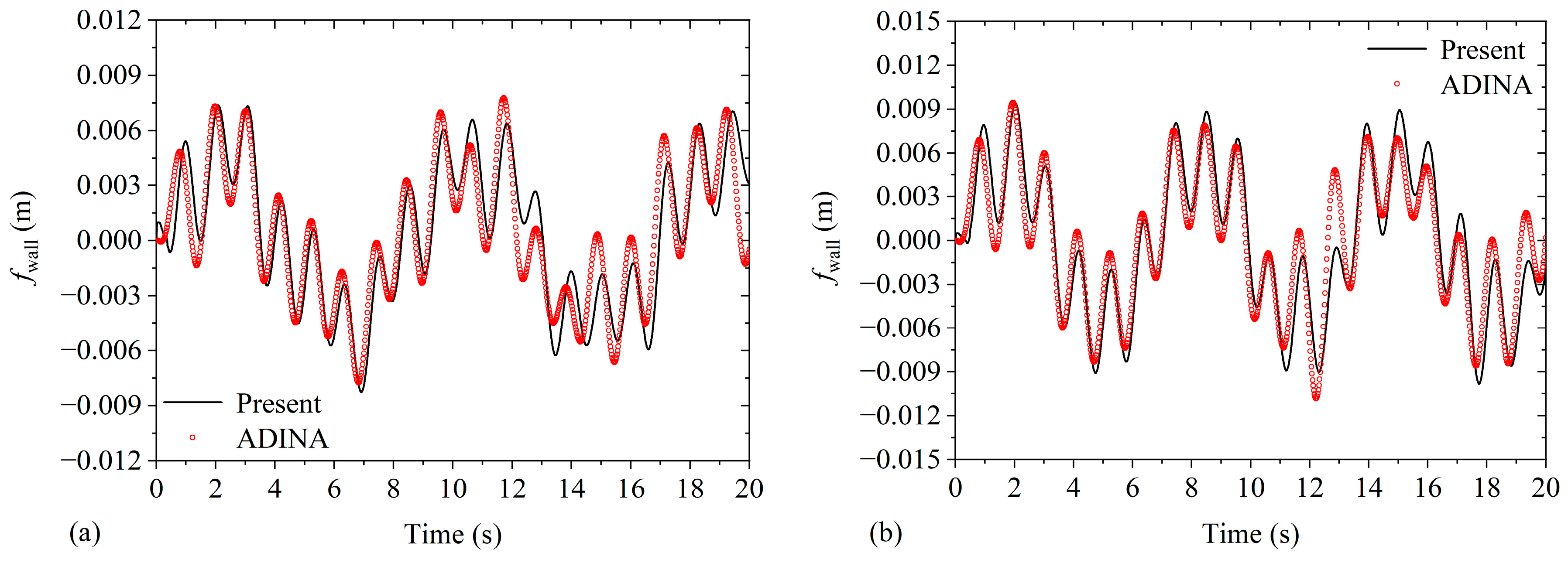
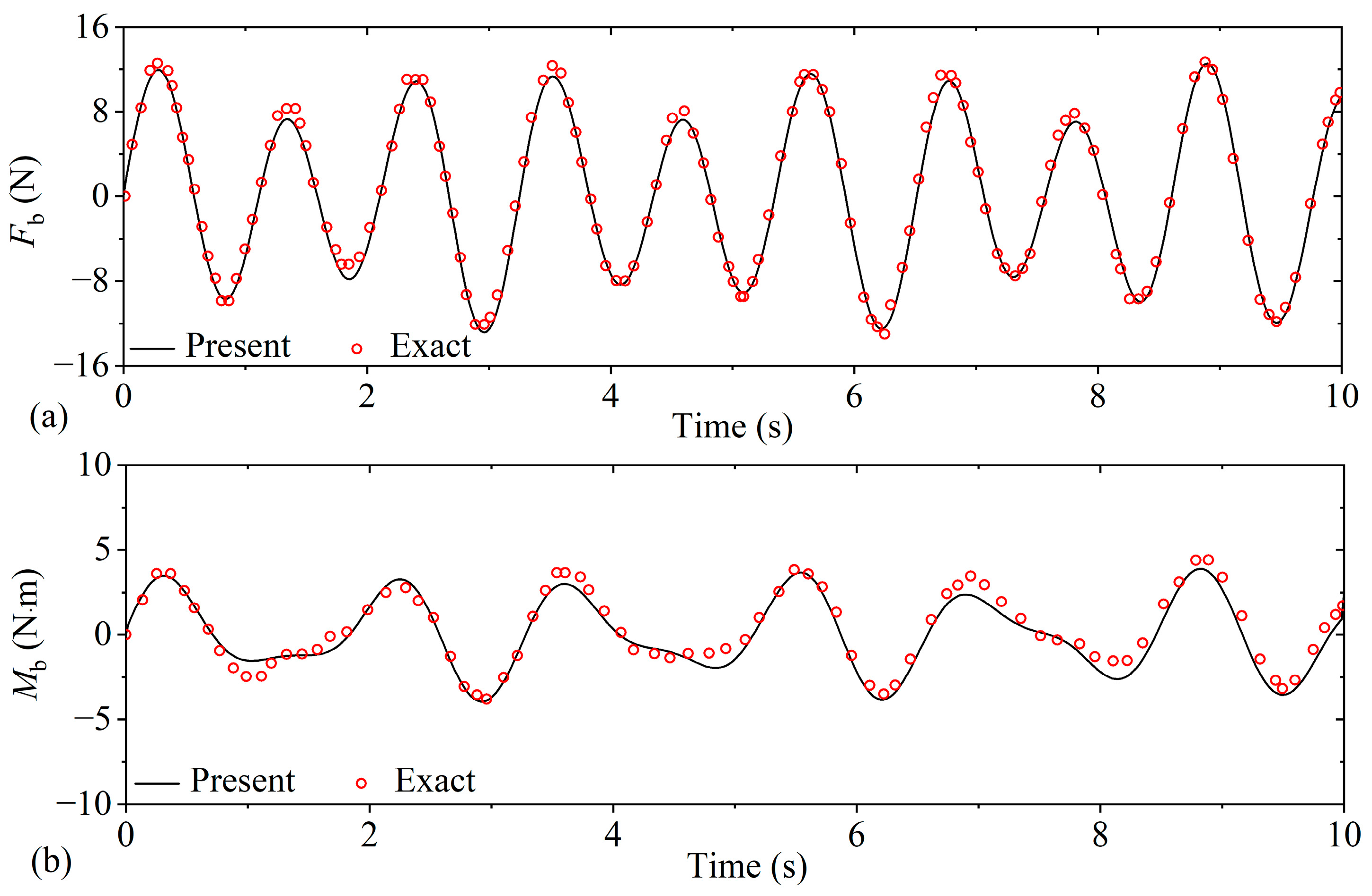
3.2. Response of the Soil–Tank System

The densities of soil, tank, and base are, respectively, 2000 kg/m3, 7800   kg / m 3 , and 2500   kg / m 3 in the present analysis. The tank heights are equal to 1.2H. The tank thickness is 0.003R2. The circular base thickness is 0.05H. By introducing artificial interfaces, Wang et al. [22] acquired exact results of linear sloshing responses of the rigid cylindrical container with an annular baffle on a rigid foundation under horizontal excitation. Figure 7 illustrates the sloshing displacement at wall fwall between the present and exact results on a rigid foundation for the baffle inner radius γ = 0.4 ,   0.6 ,   0.8 with R 2 = 0.508 m, β 1 = 0.7, β 2 = 1.0 , and V s = 1000   m / s under the excitation u ¨ g ( t ) = 0.001 ϖ 2 sin ϖ t   ( ϖ = 5.811   rad / s ) .  Figure 8 depicts the base shear F b and base moment M b between the present and exact results on a rigid foundation for β 1 = 0.9, β 2 = 1.0, γ = 0.6 and V s = 1000   m / s under the same excitation. It is clear from Figure 7 and Figure 8 that present reduced results with V s = 1000   m / s (representing rigid soil) show excellent agreement with the available exact results under a rigid foundation, which implies the feasibility of the present method. In Figure 9, the time histories of the present sloshing displacement at wall fwall under various vs. are compared, with linear numerical results [42] under rigid foundation for β 1 = 0.2, β 2 = 1.0, γ = 0.4 , R 2 = 0.508 m, and u ¨ g ( t ) = 0.002 ϖ 2 sin ϖ t   ( ϖ = 5.8   rad / s ) . It is clear from Figure 9 that the dynamics of the tank with β 1 = 0.2 keep consistent with those without a baffle due to the fact that the effects of the baffle approaching the bottom are almost negligible [42]. The solution under a flexible foundation is similar to the linear numerical result [42] under a rigid foundation. The result also implies that soils with different stiffnesses have little effect on the sloshing height.
Consider two cylindrical tanks supported on a surface foundation. The present results of fwall are compared with finite-element results from the ADINA model to further verify the correctness and effectiveness of the theoretical model. The parameters are given as follows: R 21 = R 22 = 10 m, β 11 = β 12 = 0.8, γ 1 = γ 2 = 0.5, r s = 25 m, and V s = 300   m / s . The liquid heights are β 21 = 0.5 for the broad tank and β 22 = 1.0 for the slender tank. In Figure 10, the analysis type of the ADINA structure is dynamic implicit. The potential interfaces are adopted to simulate boundary conditions of liquid. The three-dimensional linear potential-based element of liquid using 8064 elements and the three-dimensional solid element using 17,780 elements are employed to imitate the liquid domain and soil, respectively. It produces, theoretically, responses free from boundary effects. Meanwhile, taking the radiation damping into account if considering an infinite horizontal extent of the soil domain, however, induces heavy computational expense. If considering the smaller width of the soil domain, the computational accuracy of the system responses cannot be ensured [43]. According to the available literature [44], the soil domain width is suggested to be about 8–10 times the foundation width. Therefore, the soil domain is founded with a 500 m width. The boundary of the soil is defined by the infinite region. The first third of the convective sloshing frequencies compared with the finite-element results are presented in Table 3. It is clear that the maximum relative error for the first third of the sloshing frequencies is −3.18%. Figure 11 illustrates the sloshing displacements at walls fwall of the two tanks in comparison with numerical solutions under V s = 300 m/s and the external excitation u ¨ g ( t ) = 0.001 ϖ 2 sin ϖ t   ( ϖ = 5.811   rad / s ) . The relative errors for the maximum sloshing displacement between present and numerical solutions are 5.27 % for the broad tank and 0.32 % for the slender tank, respectively. The good agreement between the present results and the finite-element results in Table 3 and Figure 11 indicates that the present method can be used to basically characterize the dynamics of the system with acceptable precision.

4. Parameter Analysis

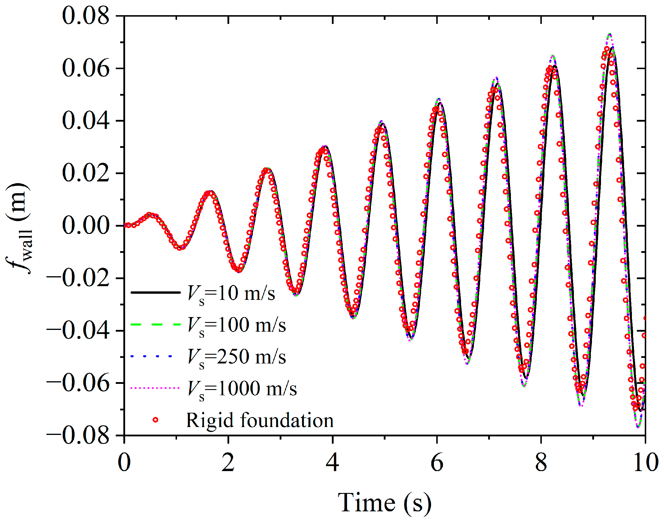
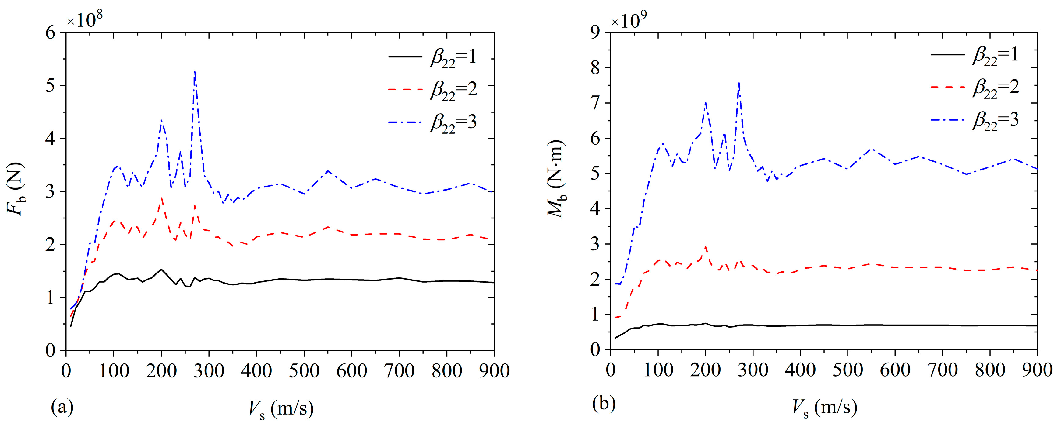
4.1. The Effect of Soil

The parameters of the two tanks are given as follows in this section: R 21 = R 22 = 15   m ,   β 11 = β 12 = 0.7 ,   γ 1 = γ 2 = 0.6 ,   β 21 = 0.5 , β 22 = 1.0 , and r s = 37.5   m . The first two convective frequencies of sloshing ω 11 C and ω 12 C of broad and slender tanks for V s are depicted in Table 4. The results imply that soft soil has little effect on the convective frequencies of two storage tanks. Furthermore, with the increase in V s , the convective sloshing features of the tanks on soft soil approach the characteristic results of the tanks on rigid soil. Figure 12 illustrates the horizontal impulsive frequency ω h I and rotational impulsive frequency ω r I for the base versus the shear-wave velocity under different liquid heights. It is clear that the impulsive frequency keeps the linear increase with the growth of V s .
Table 5 gives the detailed near-fault (NF) and far-fault (FF) seismic records. Figure 13 depicts variations of the base shear F b and base moment M b versus V s when tanks are subjected to NF seismic motion in Table 5. The liquid heights of broad and slender tanks are β 21 = 0.5 and β 22 = 1 ,   2 ,   3 , respectively. It is observed that the effect of softer soil with lower V s on the base response is greater than that of stiffer soil with the larger V s ( V s 400   m / s ) on the base response. The maxima of F b and M b both appear at V s equal to 270 m/s for β 22 = 3 . Furthermore, the larger nondimensional liquid height characteristically accompanies the larger base response for the same V s in Figure 13.

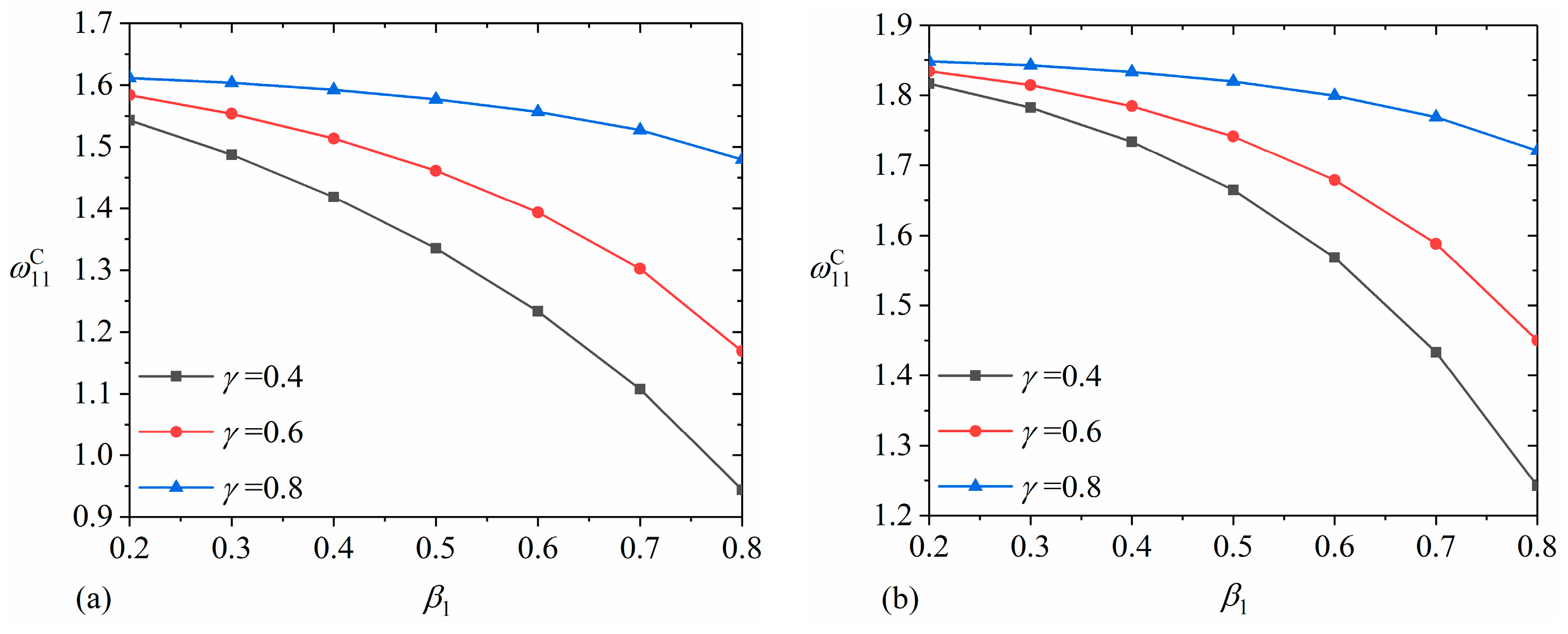
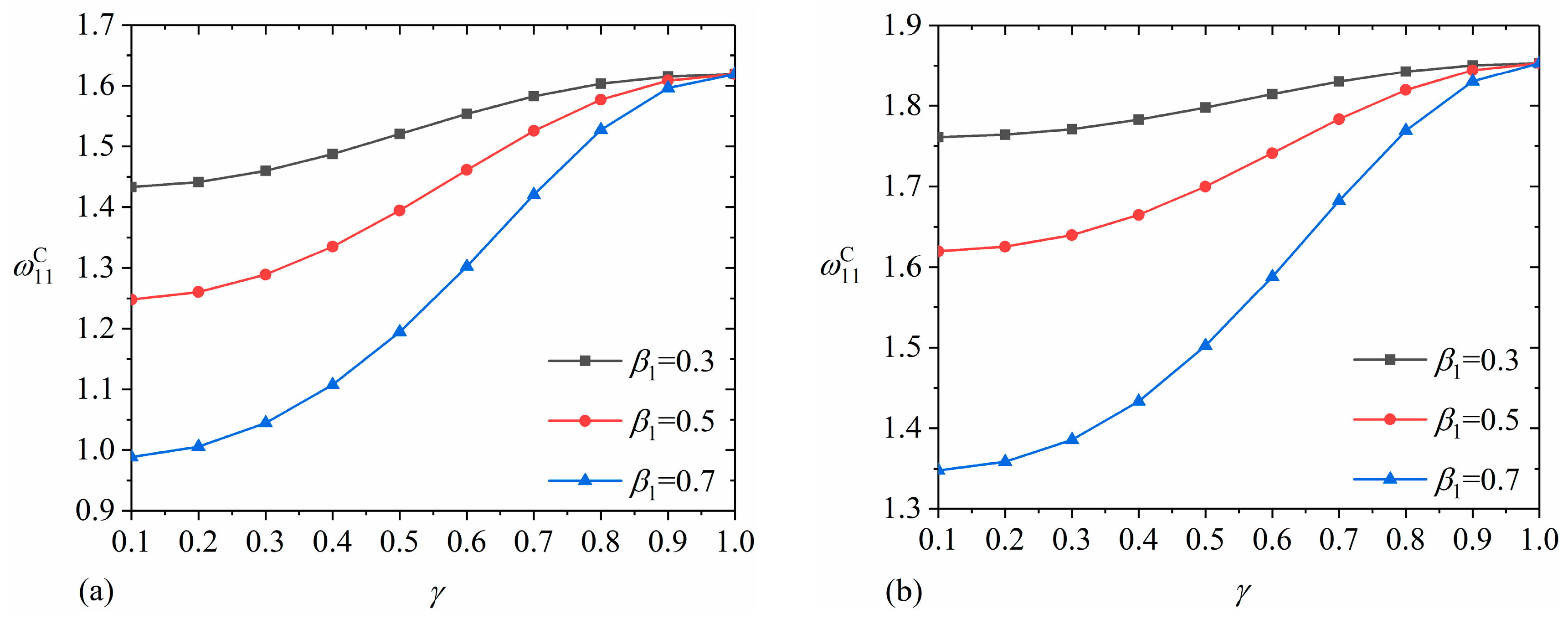
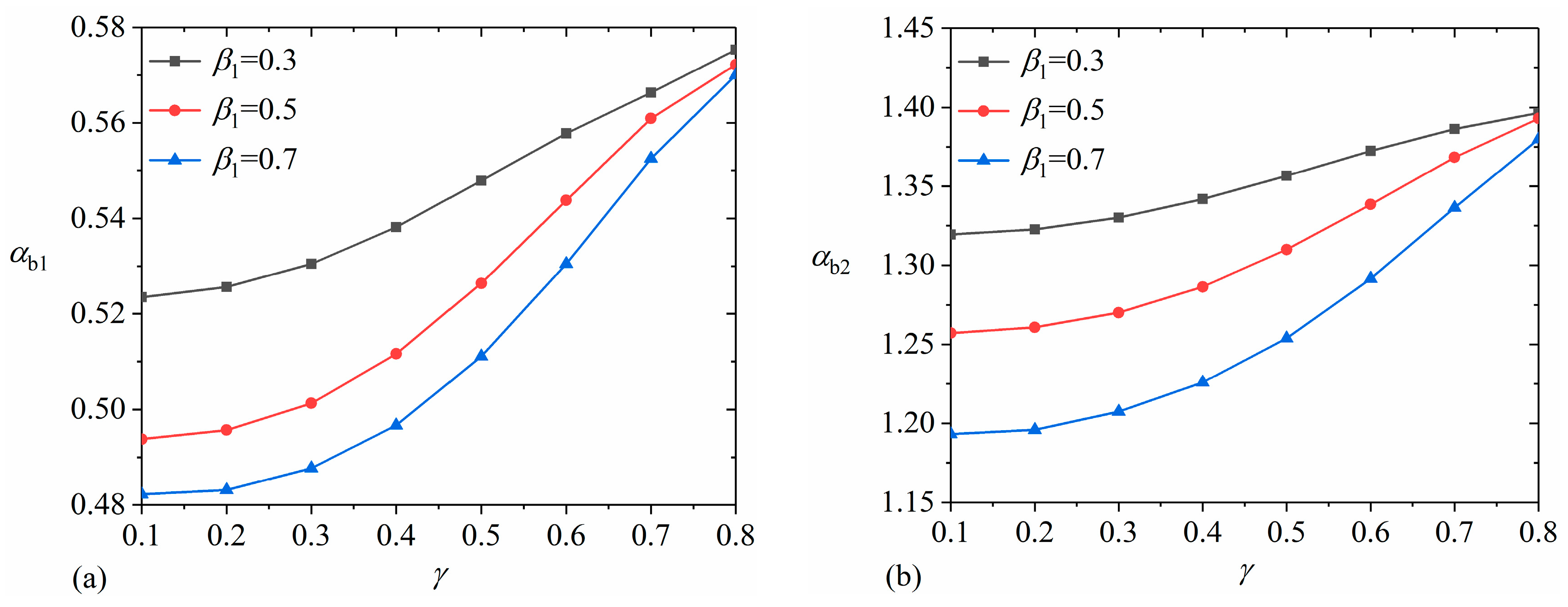
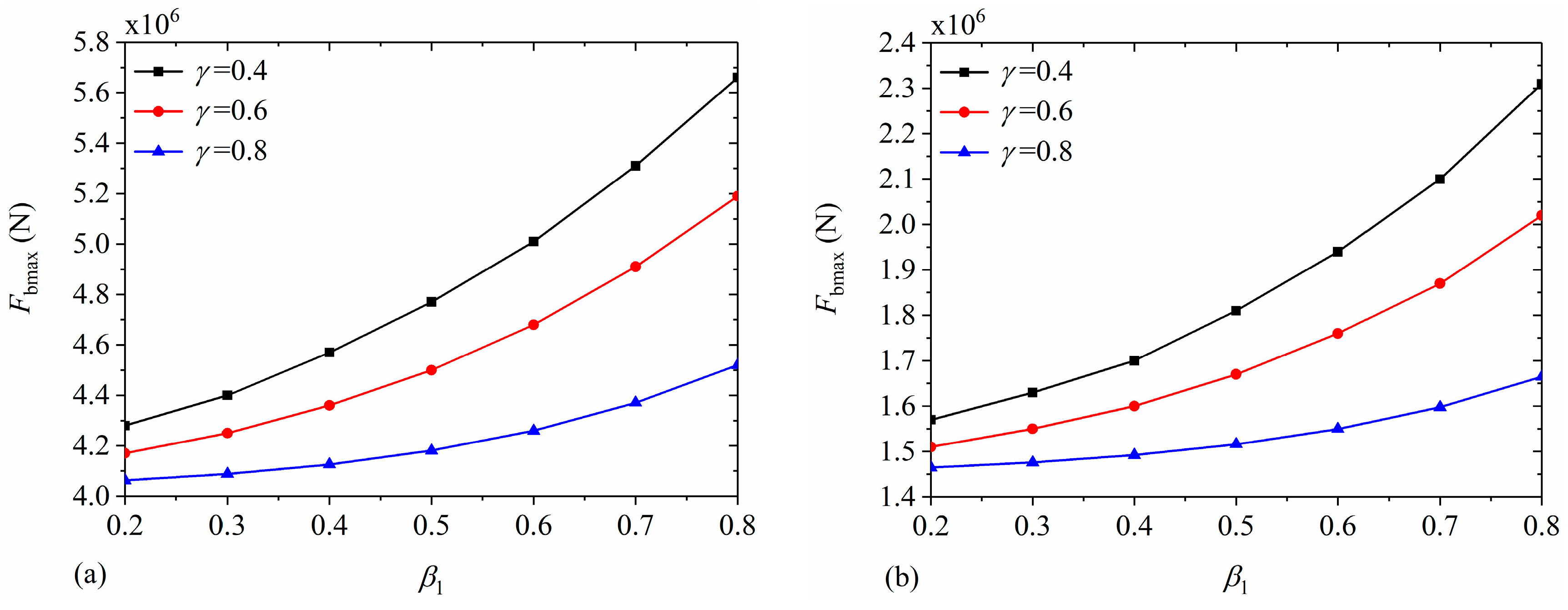
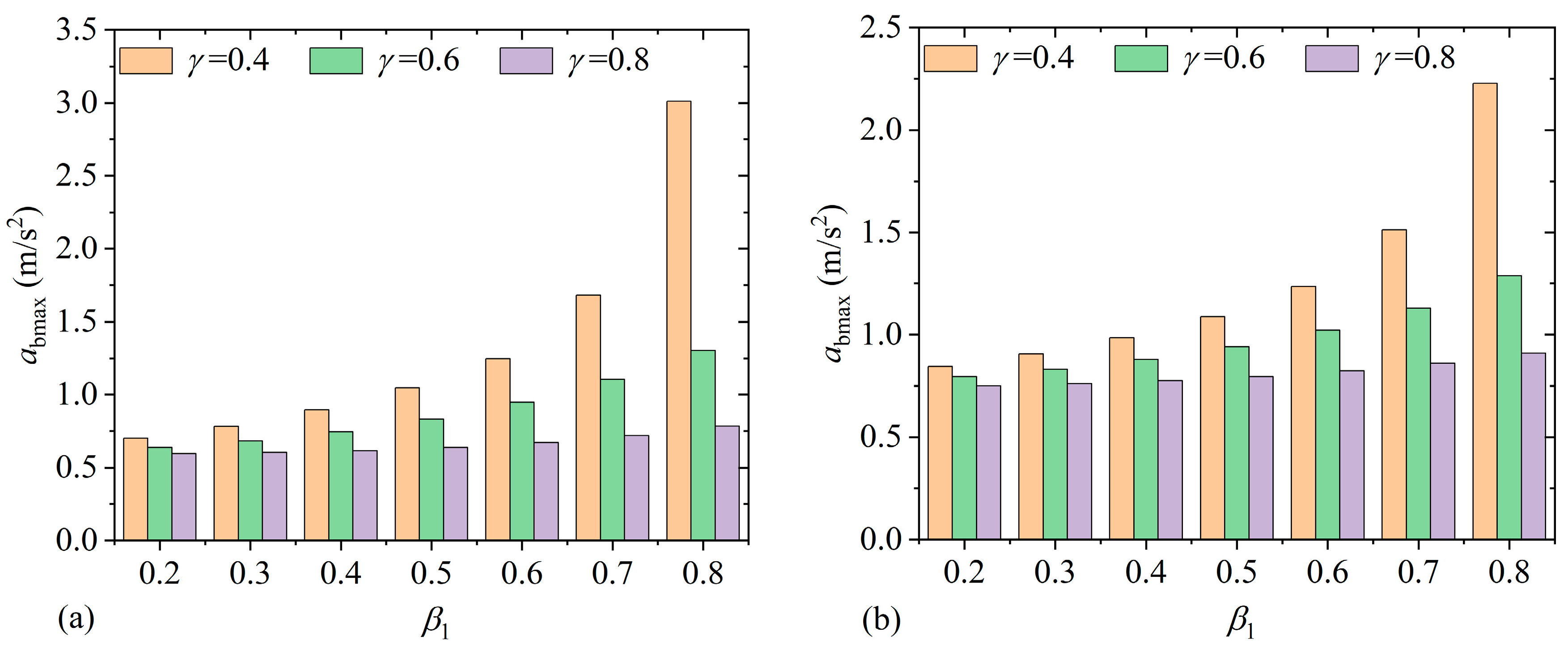
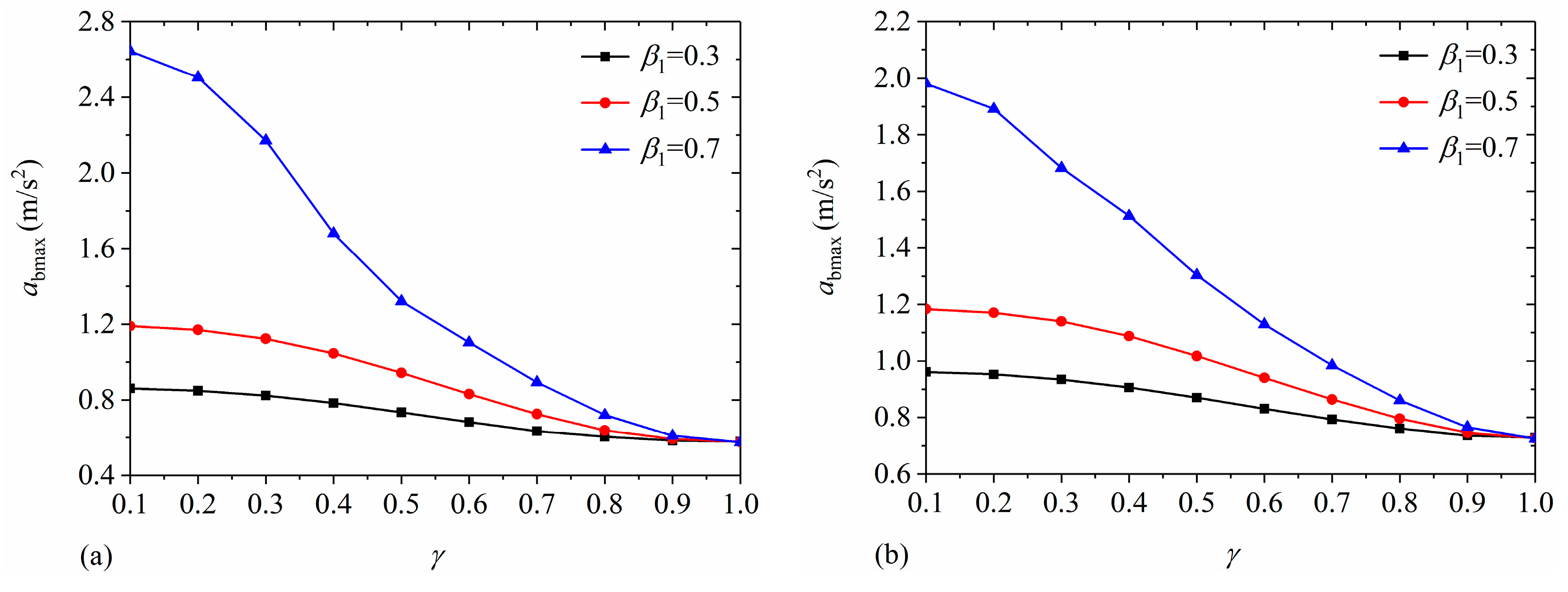
4.2. The Effect of Baffle

If not specified separately in this section, the liquid heights are β 21 = 0.5 and β 22 = 1.0 , with V s = 200   m / s and r s = 12.5   m , respectively. The inner radiuses of the two tanks are considered as R 21 = R 22 = 5   m .  Figure 14 depicts first-order convective sloshing frequencies ω 11 C of broad and slender tanks versus different baffle heights β 1 with γ = 0.4 ,   0.6 ,   0.8 . It is seen in Figure 14 that, by increasing the nondimensional baffle height, ω 11 C both decline in two storage tanks. Figure 15 shows first-order convective sloshing frequencies ω 11 C of broad and slender tanks under different baffle inner radiuses γ , with β 1 = 0.3 ,   0.5 ,   0.7 . In Figure 15, ω 11 C both improve with the growth of the nondimensional baffle inner radius of broad and slender tanks. Figure 16 reveals the time history of fwall for β 11 = β 12 = 0.7 and γ 1 = γ 2 = 0.8 subjected to the excitation frequencies u ¨ g ( t ) = 0.001 ϖ 2 sin ϖ t   ( ϖ = 1.6   rad / s ,   3.0   rad / s ,   5.8   rad / s ) . The first convective sloshing frequencies ω 11 C of the broad tank and the slender tank are, respectively, 1.5272 rad/s and 1.7691 rad/s. The results in Figure 16 imply that resonance of liquid sloshing could occur when the excitation frequencies approach sloshing frequencies since damping effects are neglected in the present analysis.
α b 1 is defined as the ratio of the maximum rocking component of F b to the horizontal one. α b 2 is defined as the ratio of the maximum rocking component of M b to the horizontal one. The utilized horizontal excitation is u ¨ g ( t ) = 0.001 ϖ 2 sin ϖ t   ( ϖ = 5.811   rad / s ) .  Figure 17 depicts the dynamic response results of α b 1 and α b 2 for the baffle height β 1 with γ = 0.4 ,   0.5 ,   0.6 and R 21 = R 22 = 0.508   m . It is observed that, by increasing the nondimensional baffle location, α b 1 declines first and then increases slightly, indicating the non-monotonic change. With the growth of the dimensionless height of the annular baffle, α b 2 declines monotonically. Figure 18 shows the dynamic response results of α b 1 and α b 2 for the radius of the annular rigid baffle γ , with β 1 = 0.3 ,   0.5 ,   0.7 and R 21 = R 22 = 0.508   m . It is observed that, with the growth of the inner radius, α b 1 and α b 2 both increase monotonically.
The influences of the baffle height and inner radius on system responses are investigated undergoing NF and FF earthquake excitations. Figure 19 and Figure 20 give influences of the baffle height on the maximum value of the base shear F bmax and moment M bmax with γ = 0.4 ,   0.6 ,   0.8 , respectively. It is observed that, by improving the nondimensional baffle height, the maximum base shear increases; however, the maximum base moment first declines and then increases. Moreover, the maximum base shear and moment under NF earthquake excitation are greater than those under FF earthquake excitation. Figure 21 illustrates the maximum value of the horizontal relative acceleration of the base a bmax for the nondimensional baffle height. The result shows that a bmax increases with the increase of the nondimensional baffle height.
Consider the nondimensional baffle heights of two tanks as β 1 = 0.3 ,   0.5 ,   0.7 Figure 22 depicts the influences of the baffle’s inner radius γ on the maximum base shear F bmax subjected to NF and FF seismic excitations. The result implies that F bmax diminishes with the growth of the nondimensional inner radius. Furthermore, the maximum base shear under NF seismic excitation is larger than that under FF seismic excitation owing to the great amplitude in the lower frequency range in terms of the power spectral density of NF seismic records. Accordingly, more attention should be paid to the structure dynamics in the vicinity of the seismic mobile moving fault. Figure 23 shows a bmax for the nondimensional baffle radius. It is observed that a bmax declines with the growth of the baffle radius.

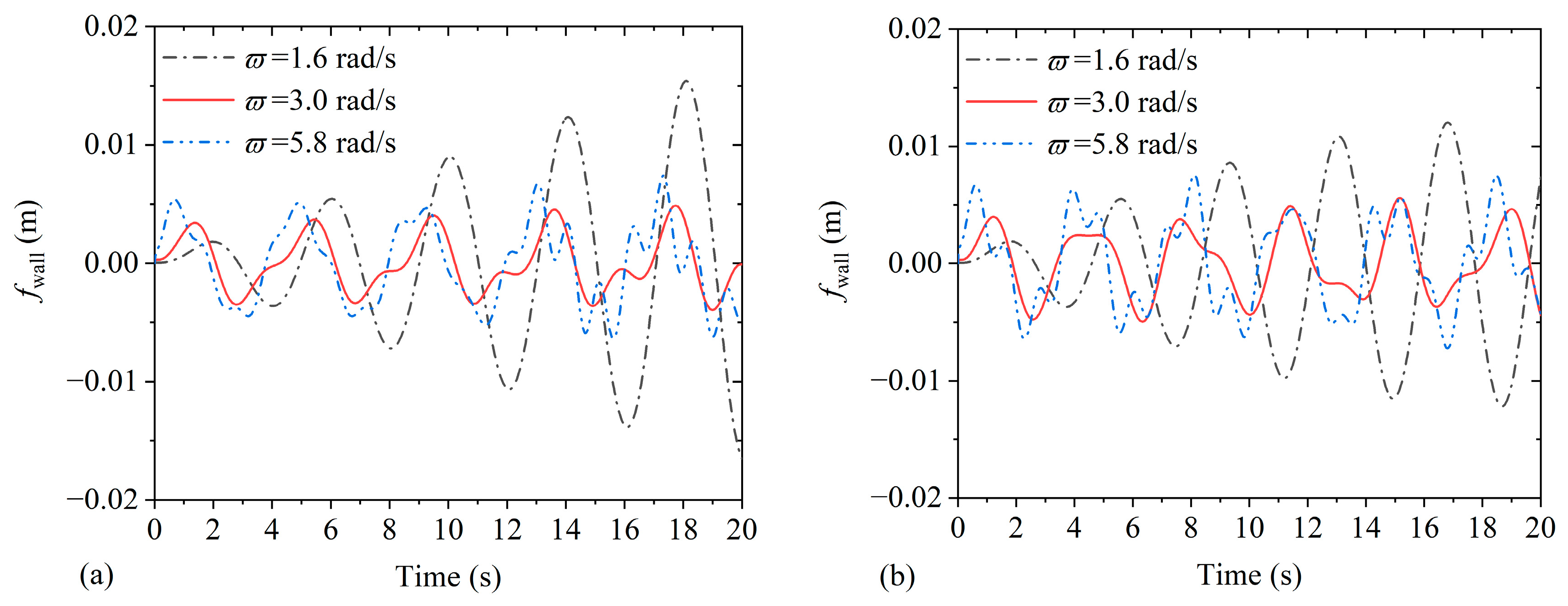
4.3. The Effect of Liquid Height

Consider the parameters of two tanks supported on the same circular surface foundation in this section to be R 21 = R 22 = 15   m ,   β 11 = β 12 = 0.8 ,   γ 1 = γ 2 = 0.7 , V s = 200   m / s , and r s = 37.5   m .  Figure 24 illustrates the calculation results of the horizontal impulsive frequency ω h I and the rotational impulsive frequency ω r I for β 21 and β 22 . In Figure 24a, the liquid height is β 22 = 1.0 . In Figure 24b, the liquid height is β 21 = 0.5 . It is clear that ω h I and ω r I decline with the increase in the liquid height. Figure 25 illustrates the maxima of the sloshing displacement at wall fmax of two cylindrical tanks for non-dimensional liquid heights β 21   ( β 22 = 1.0 ) and β 22   ( β 21 = 0.5 ) . The horizontal excitation considered is u ¨ g ( t ) = 0.001 ϖ 2 sin ϖ t   ( ϖ = 5.811   rad / s ) . It is observed that with the increase in liquid heights of the two tanks, fmax both increase. Furthermore, the maximum value of the sloshing displacement of the slender storage tank is greater than that of the broad storage tank.
Figure 26 gives time histories of the base shear F b and base moment M b for β 21 = 0.4 ,   0.5 ,   0.6 and β 22 = 1.0 under Kobe excitation. Figure 27 illustrates time histories of F b and M b for β 21 = 0.5 and β 22 = 1.0 ,   1.2 ,   1.4 under NF excitation. It is clear that F b and M b both increase with the growth of liquid heights of each tank. The values of the maximum F b and M b for β 21 = 0.6 increase 32.71% and 19.14% in comparison with those of β 21 = 0.4 , respectively. The values of the maximum F b and M b for β 22 = 1.4 increase 33.56% and 81.45% in comparison with those of β 22 = 1.0 , respectively. Figure 28 shows the normalized maximum base shear F bmax / M f g and the normalized maximum base moment M bmax / 0.5 M f g H versus the dimensionless liquid height β 2 with V s = 150   m / s ,   200   m / s ,   250   m / s under NF excitation. M f stands for the total liquid mass. It is observed that the normalized base responses show the non-monotonical variation with the growth of the dimensionless liquid height. In addition, non-monotonical change occurs at the larger liquid height in terms of the greater soil shear-wave velocity.

5. Discussion

In this study, dynamic characteristics and responses of multiple cylindrical liquid storage tanks with baffles and resting on soil undergoing any type of horizontal excitation are examined. The influences of soil and baffle parameters on dynamic performances are considered in the investigation.
In this study, sloshing resonance could occur if excitation frequencies approach sloshing frequencies since damping effects are neglected. Thus, installing an internal baffle is an effective measure to mitigate sloshing. The baffle’s existence could reduce the sloshing amplitude of the liquid surface, which is consistent with the available reports [42] seen in Figure 7 from Section 3.2.
In this study, good agreement between the present results and the numerical results indicates that the present method can be utilized to basically characterize the dynamics of the system with acceptable accuracy, which is considered the first novelty of the present investigation.
In addition, in terms of each solution to the dynamic responses, the simulation from the ADINA numerical model takes approximately 486 s on a laptop with the Intel Core i9-9900K CPU, whereas the simulation of the present model by the MATLAB procedure only takes about 11 s on the same laptop. Thus, the solution efficiency of system dynamics from the present model is 40–50 times faster than that from the ADINA model. The result implies that the present method can also provide high calculation efficiency when studying the dynamic behaviors of the coupling system, which is the second novelty of the present investigation.

6. Conclusions

A mechanical model is first proposed to obtain dynamic features and earthquake responses of the multiple tanks with a single baffle and supported on a surface foundation. Combined with the substructure method, a mass-spring theoretical model for sloshing in each rigid circular cylindrical tank based on the semi-analytical liquid subdomain partition technique is assembled with the soil lumped-parameter model representing horizontal, rocking, and coupling dynamic impedance functions. The proposed model simplifies the dynamics of the complicated system with high calculation efficiency and acceptable accuracy, which is a novelty of the present study. The present dynamic properties and responses of the baffled tanks on rigid and soft soil foundations are compared with the exact results and numerical results, including those from ADINA to prove the reliability and applicability of the coupling model. Effects of the soil shear-wave velocity, baffle height, and size, as well as liquid height on system dynamics undergoing near-fault and far-fault horizontal seismic motions, are investigated.
(1)
The impulsive frequency keeps increasing linearly with the increase in soil stiffness. Soils with different stiffnesses have little influence on the sloshing height; however, soil–structure interaction can exert a remarkable effect on the base response of multiple tanks. The base shear and moment both vary non-monotonically with the growth of the soil’s stiffness;
(2)
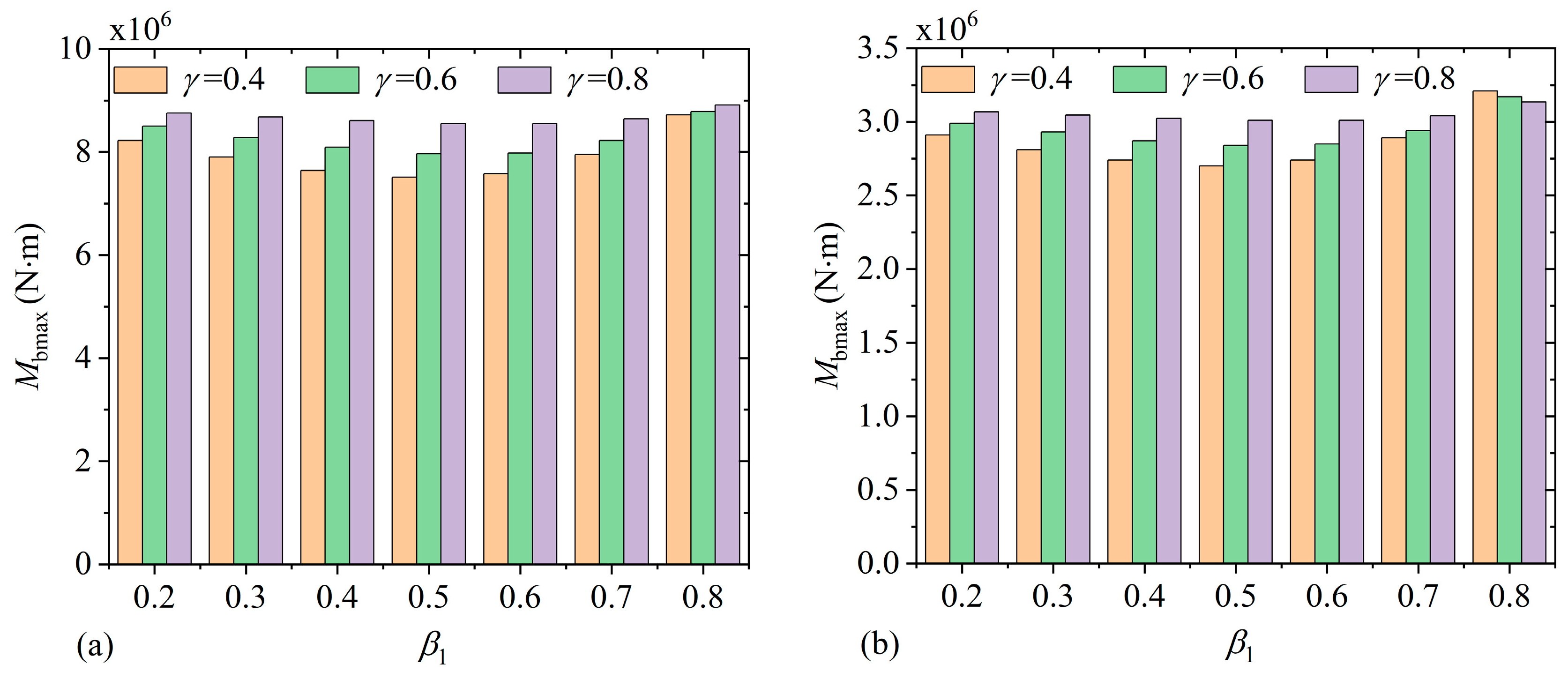
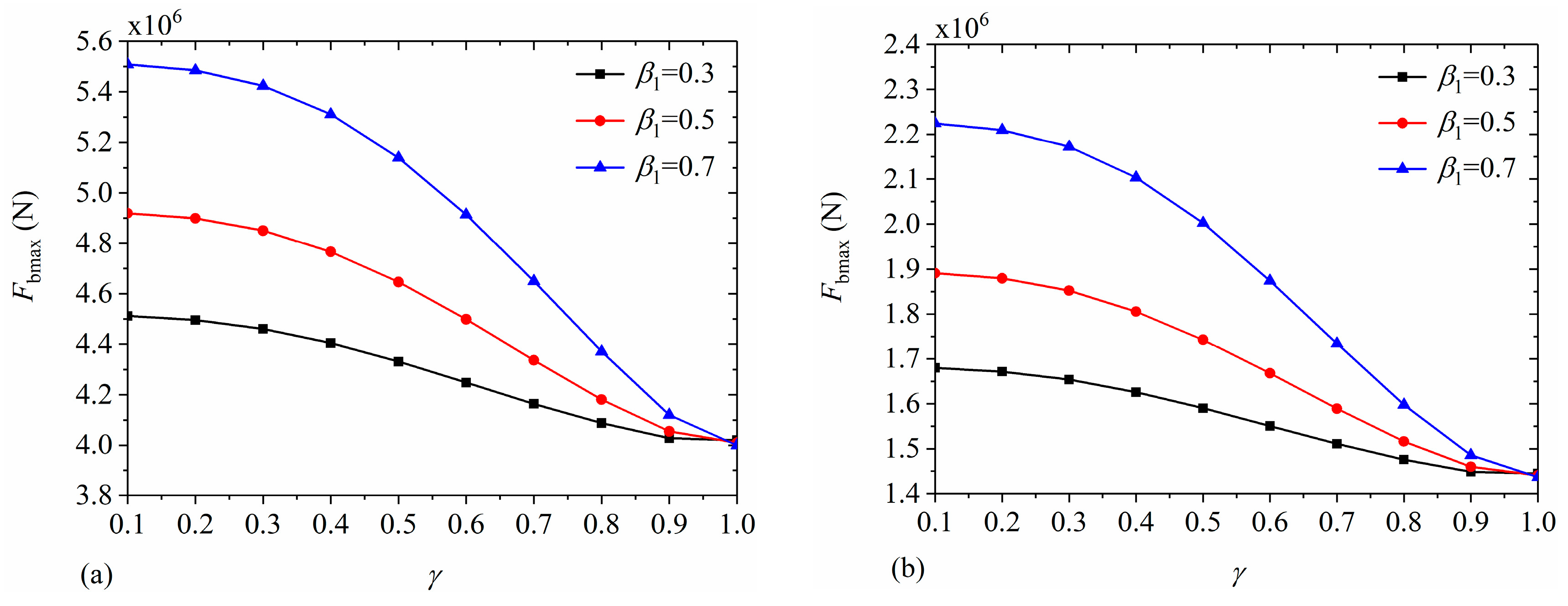
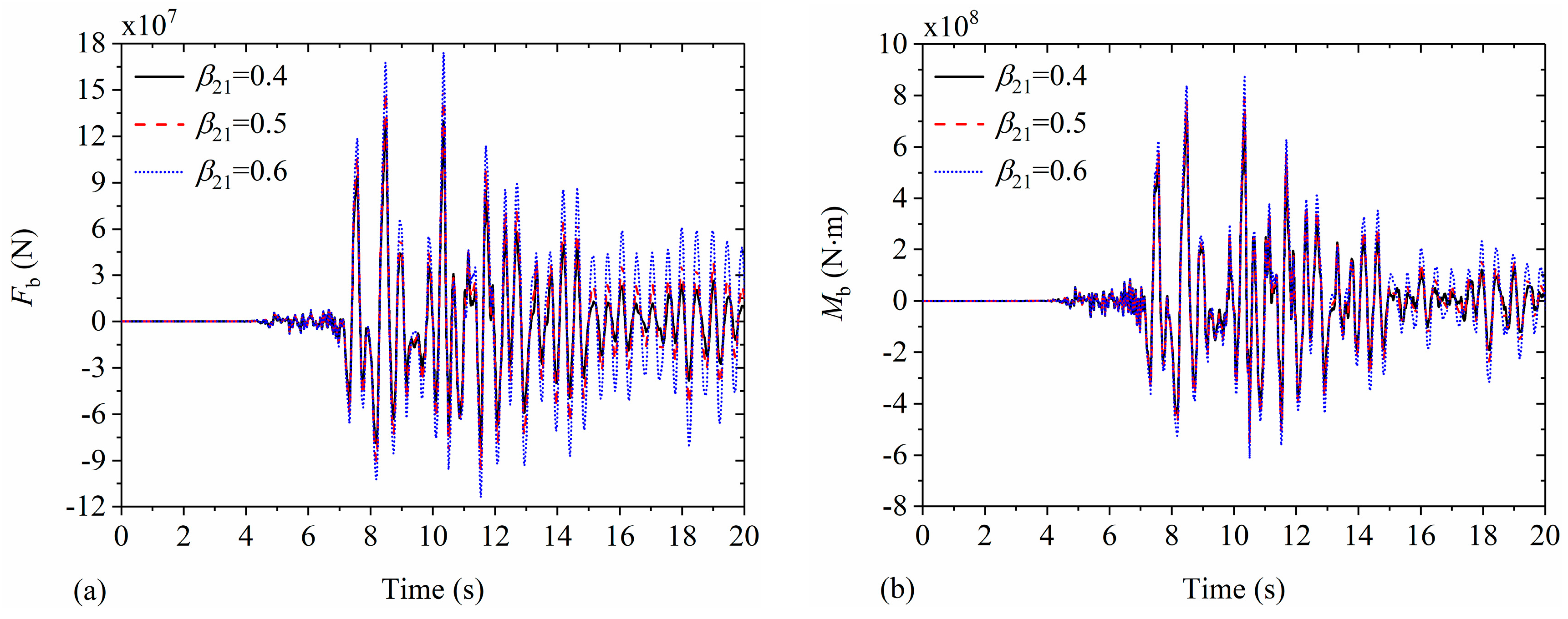
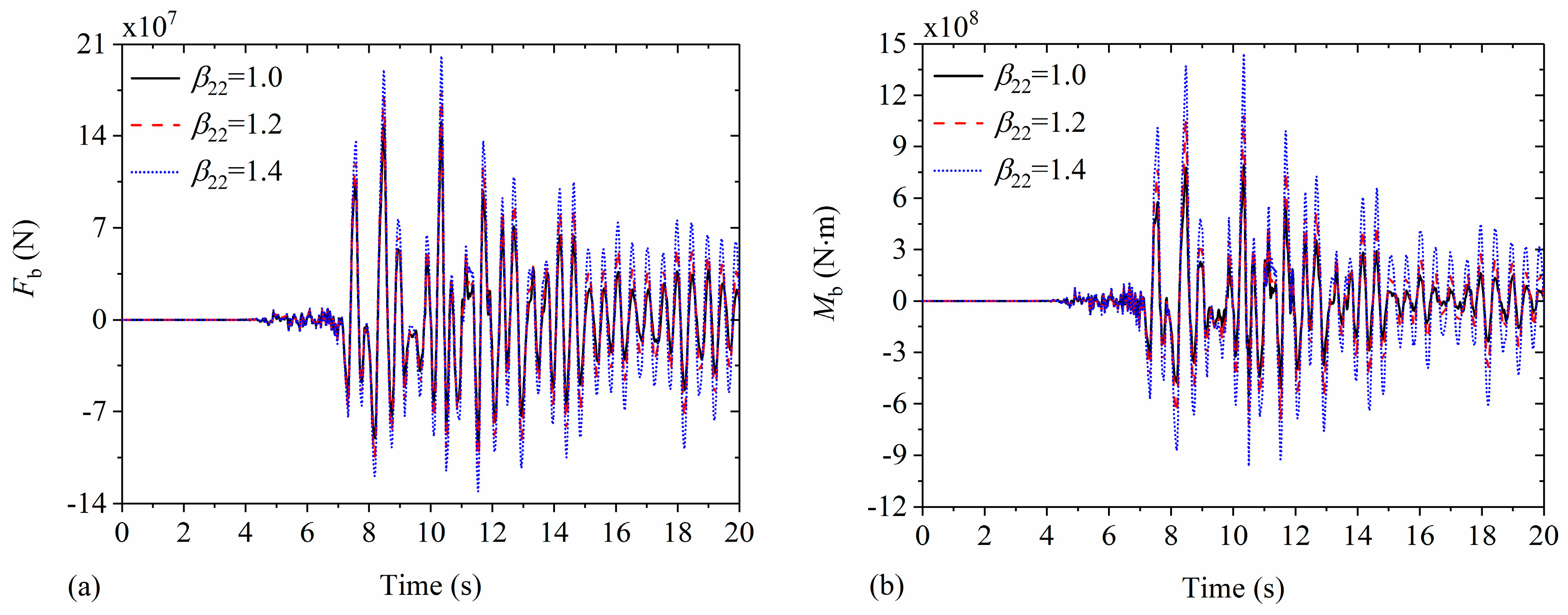
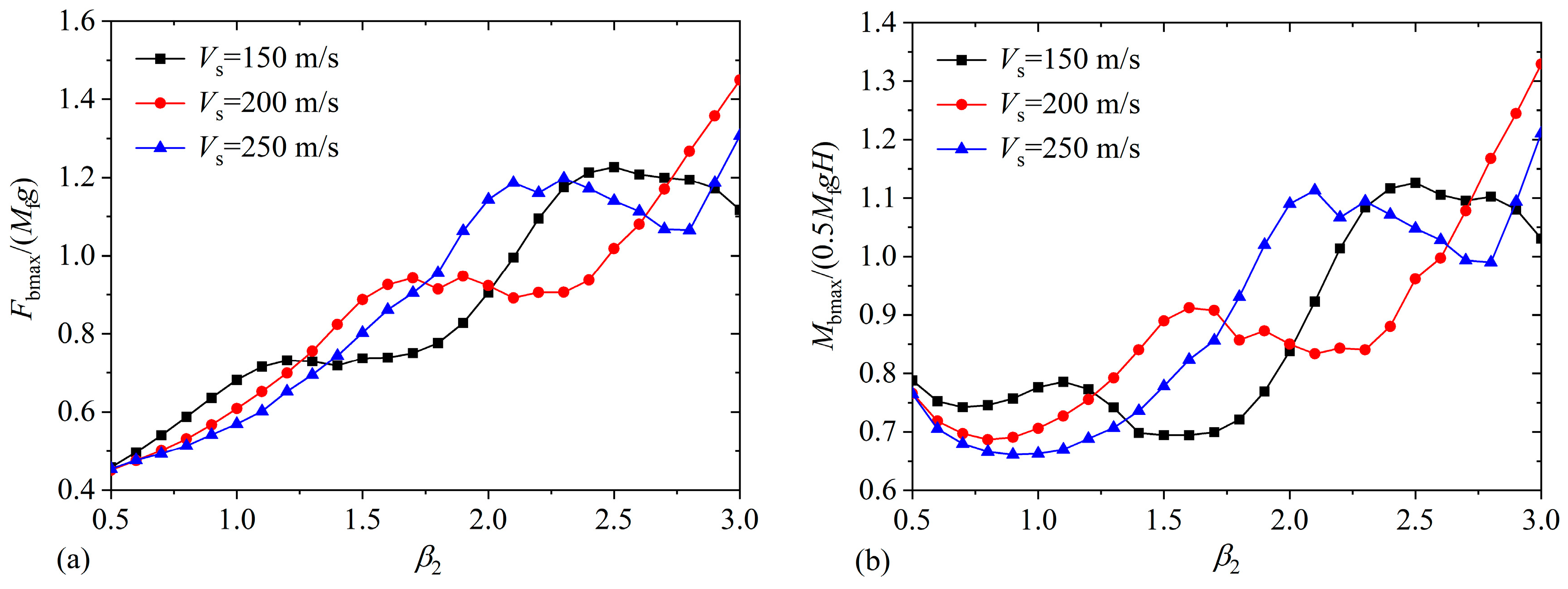
By increasing the nondimensional baffle location, the maximum base shear increases; however, the maximum base overturning moment varies non-monotonically. The maximum base shear and moment under near-fault seismic excitation are greater than those under far-fault seismic excitation;
(3)
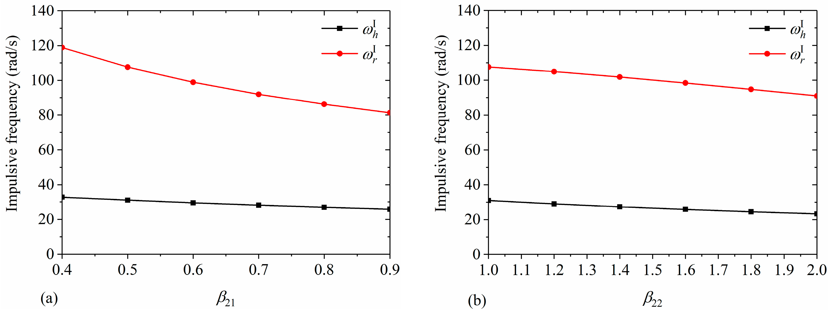
The impulsive frequencies of the base diminish with the growth of the nondimensional liquid height. The non-monotonical variation for the normalized base responses occurs at the larger liquid height in terms of the greater soil shear-wave velocity. The results show that the maximum base shear and moment subjected to near-fault seismic activity could increase, respectively, 33.56% and 81.45% with the growth of the liquid height of the slender tank on soft soil.
In this research, the movement equations of rigid bodies of a group of tanks partially filled with liquid are equivalent to those connected to mass-spring oscillators. From the perspective of the application, the mechanical model of the original system can be more informative when studying each element’s role in the system. In terms of the large liquid storage systems built on soft foundations, it is essential to account for soil–tank–liquid–baffle interaction to obtain the seismic design with acceptable accuracy. The present method is limited to the dynamic analysis of influences of the rigid annular baffle in multiple rigid tanks resting on soft soil. The method will be modified in future research investigating the influences of the elastic baffle and tank wall, which is more in line with practical engineering.

Author Contributions

Methodology, Y.S.; Software, Z.Z.; Validation, Y.S.; Formal analysis, X.M.; Investigation, X.M.; Resources, Z.G.; Data curation, Z.Z.; Writing—original draft, Y.S.; Writing—review & editing, Z.G., J.W. and D.Z.; Visualization, Z.Z.; Project administration, D.Z.; Funding acquisition, Z.G., J.W. and D.Z. All authors have read and agreed to the published version of the manuscript.

Funding

This work was supported by the National Natural Science Foundation of China (grant numbers 51978336 and 11702117) and the Nantong City Social Livelihood Science and Technology Project (grant number MS22022067). The APC was funded by Scientific Research Starting Foundation for the High-Level Person (grant number 135422633010).

Data Availability Statement

The datasets used and/or analyzed during the current study are available from the corresponding author upon reasonable request.

Conflicts of Interest

The authors declare that there are no conflicts of interest.

Appendix A

The Equations (28)–(31) can be derived as the following forms:
F w a l l m = n = 1 q ¨ n m ( t ) A 1 n m ρ π R 2 m 2 H m u ¨ ( t )
M w a l l m = n = 1 q ¨ n m ( t ) B 1 n m 1 2 ρ π R 2 m 2 H m 2 u ¨ ( t )
M b o t t o m m = n = 1 q ¨ n m ( t ) C 1 n m 1 4 ρ π R 2 m 4 u ¨ ( t )
M b a f f l e m = n = 1 q ¨ n m ( t ) D 1 n m
in which
A 1 n m = ρ π R 2 m 0 h m Φ 1 n m 3 ( R 2 m , z ) d z + h m H m Φ 1 n m 1 ( R 2 m , z ) d z ,
B 1 n m = ρ π R 2 m 0 h m z Φ 1 n m 3 ( R 2 m , z ) d z + h m H m z Φ 1 n m 1 ( R 2 m , z ) d z ,
C 1 n m = ρ π 0 R 1 m Φ 1 n m 4 ( r , 0 ) r 2 d r + R 1 m R 2 m Φ 1 n m 3 ( r , 0 ) r 2 d r ,
D 1 n m = ρ π R 1 m R 2 m Φ 1 n m 1 ( r , h m ) r 2 d r R 1 m R 2 m Φ 1 n m 3 ( r , h m ) r 2 d r .

Appendix B

The mass matrix M has the following form:
M = M ¯ A * T 0 ( m = 1 V N m ) × N s A * H * T 0 ( m = 1 V N m ) × N s A * M h 0 N s M h r 0 N s 0 N s × ( m = 1 V N m ) 0 N s T 0 N s × N s 0 N s T 0 N s × N s A * H * M h r 0 N s M r 0 N s 0 N s × ( m = 1 V N m ) 0 N s T 0 N s × N s 0 N s T 0 N s × N s ( m = 1 V N m + 2 N s + 2 )                           × ( m = 1 V N m + 2 N s + 2 ) ,
where M ¯ ( m = 1 V N m ) × ( m = 1 V N m ) = M 1 n 1 * N 1 × N 1       0             M 1 n m * N m × N m             0       M 1 n V * N V × N V ,
M 1 n m N m × N m = d i a g ( A 11 m ,   ,   A 1 n m ,   ,   A 1 N m m ) ,   A * = A 1 n 1 N 1 ,   ,   A 1 n m N m ,   ,   A 1 n V N V ,
A * H * = A 1 n 1 H 1 n 1 * N 1 ,   ,   A 1 n m H 1 n m N m ,   ,   A 1 n V H 1 n V * N V ,
M h = m = 1 V n = 1 N m A 1 n m + m = 1 V A 10 m + M t ,   M h r = m = 1 V n = 1 N m A 1 n m H 1 n m + m = 1 V A 10 m H 10 m + M t y t ,
M r = m = 1 V n = 1 N m A 1 n m H 1 n m 2 + m = 1 V A 10 m H 10 m 2 + M t y t 2 + J t ,
where A 1 n m * and H 1 n m * are the n th order convective mass and its location in the m th tank, respectively. A 10 m * and H 10 m * are the impulsive mass and its location in the m th tank, respectively. Mt is the total mass of the tanks and base. yt and Jt denote the barycenter and the moment of inertia for tanks with the base.
The stiffness matrix K has the form:
K = K *   0   K h K h r 0 K h r K r ( m = 1 V N m + 2 N s + 2 ) × ( m = 1 V N m + 2 N s + 2 ) ,
where K * ( m = 1 V N m ) × ( m = 1 V N m ) = K 1 n 1 * N 1 × N 1       0             K 1 n m * N m × N m             0       K 1 n V * N V × N V ,
K h ( N s + 1 ) × ( N s + 1 ) = k s h + k 1 h k 1 h         0 k 1 h k 1 h + k 2 h k 2 h                         k j 1 h k j 1 h + k j h k j h                         k N s 1 h k N s 1 h + k N s h k N s h 0         k N s h k N s h ,
K h r ( N s + 1 ) × ( N s + 1 ) = k s h r + k 1 h r k 1 h r         0 k 1 h r k 1 h r + k 2 h r k 2 h r                         k j 1 h r k j 1 h r + k j h r k j h r                         k N s 1 h r k N s 1 h r + k N s h r k N s h r 0         k N s h r k N s h r ,
K r ( N s + 1 ) × ( N s + 1 ) = k s r + k 1 r k 1 r         0 k 1 r k 1 r + k 2 r k 2 r                         k j 1 r k j 1 r + k j r k j r                         k N s 1 r k N s 1 r + k N s r k N s r 0         k N s r k N s r ,
K 1 n m * N m × N m = d i a g ( k 11 m * ,   ,   k 1 n m * ,   ,   k 1 N m m * ) , k j h = χ j h k s h , k j h r = χ j h r k s h r , k j r = χ j r k s r . k 1 n m * is the corresponding stiffness of the springs of the n th order convective mass. k s h , k s h r , and k s r are static stiffnesses of horizontal, horizontal–rocking coupling, and rocking LPMs, respectively. χ j h , χ j h r , and χ j r   ( j = 1 , ,   N s ) are stiffness coefficients of the j th degree of freedom in the corresponding LPMs, respectively.
The stiffness matrix C has the following form:
C = 0   0   C h C h r 0 C h r C r ( m = 1 V N m + 2 N s + 2 ) × ( m = 1 V N m + 2 N s + 2 ) , C h ( N s + 1 ) × ( N s + 1 ) = c s h         0   c 1 h                         c j h               0         c N s h , C h r ( N s + 1 ) × ( N s + 1 ) = c s h r         0   c 1 h r                         c j h r               0         c N s h r , C r ( N s + 1 ) × ( N s + 1 ) = c s r         0   c 1 r                         c j r               0         c N s r , c s h = σ h r s k s h V s , c j h = δ j h r s k s h V s , c s h r = σ h r r s k s h r V s , c j h r = δ j h r r s k s h r V s , c s r = σ r r s k s r V s , c j r = δ j r r s k s r V s . σ h , σ h r , and σ r represent damping coefficients at the high-frequency limit of horizontal, horizontal–rocking coupling, and rocking nested LPMs, respectively. δ j h , δ j h r , and δ j r   ( j = 1 , ,   N s ) denote the damping coefficients of the j th degree of freedom in the corresponding nested LPMs, respectively.

References

  1. Zhao, Y.; Li, H.-N.; Fu, X.; Zhang, S.; Mercan, O. Seismic analysis of a large LNG tank considering the effect of liquid volume. Shock Vib. 2020, 2020, 8889055. [Google Scholar] [CrossRef]
  2. Xiao, C.; Wu, Z.; Chen, K.; Tang, Y.; Yan, Y. Development of a water supplement system for a tuned liquid damper under excitation. Buildings 2023, 13, 1115. [Google Scholar] [CrossRef]
  3. Cheng, X.; Jing, W.; Li, D. Dynamic response of concrete tanks under far-field, long-period earthquakes. Proc. Inst. Civ. Eng. Struct. Build. 2021, 174, 41–54. [Google Scholar] [CrossRef]
  4. Xu, B.; Han, Z.; Wang, L.; Liu, Q.; Xu, X.; Chen, H. The influence of integral water tank on the seismic performance of slender structure: An experimental study. Buildings 2023, 13, 736. [Google Scholar] [CrossRef]
  5. Tsao, W.-H.; Huang, L.-H.; Hwang, W.-S. An equivalent mechanical model with nonlinear damping for sloshing rectangular tank with porous media. Ocean Eng. 2021, 242, 110145. [Google Scholar] [CrossRef]
  6. Luo, D.; Liu, C.; Sun, J.; Cui, L.; Wang, Z. Sloshing effect analysis of liquid storage tank under seismic excitation. Structures 2022, 43, 40–58. [Google Scholar] [CrossRef]
  7. Wang, J.; Zhang, Y.; Looi, D.T. Analytical H and H2 optimization for negative-stiffness inerter-based systems. Int. J. Mech. Sci. 2023, 249, 108261. [Google Scholar] [CrossRef]
  8. Bellezi, C.A.; Cheng, L.-Y.; Nishimoto, K. A numerical study on sloshing mitigation by vertical floating rigid baffle. J. Fluids Struct. 2022, 109, 103456. [Google Scholar] [CrossRef]
  9. Baghban, M.H.; Razavi Tosee, S.V.; Valerievich, K.A.; Najafi, L.; Faridmehr, I. Seismic analysis of baffle-reinforced elevated storage tank using finite element method. Buildings 2022, 12, 549. [Google Scholar] [CrossRef]
  10. Cho, I.H.; Kim, M.H. Effect of a bottom-hinged, top-tensioned porous membrane baffle on the sloshing reduction in a rectangular tank. Appl. Ocean Res. 2020, 104, 102345. [Google Scholar] [CrossRef]
  11. Wang, Z.; Han, F.; Liu, Y.; Li, W. Evolution process of liquefied natural gas from stratification to rollover in tanks of coastal engineering with the influence of baffle structure. J. Mar. Sci. Eng. 2021, 9, 95. [Google Scholar] [CrossRef]
  12. Yu, L.; Xue, M.-A.; Zhu, A. Numerical investigation of sloshing in rectangular tank with permeable baffle. J. Mar. Sci. Eng. 2020, 8, 671. [Google Scholar] [CrossRef]
  13. Wang, L.; Xu, M.; Zhang, Q. Numerical investigation of shallow liquid sloshing in a baffled tank and the associated damping effect by BM-MPS method. J. Mar. Sci. Eng. 2021, 9, 1110. [Google Scholar] [CrossRef]
  14. Zhang, Z.L.; Khalid, M.S.U.; Long, T.; Chang, J.Z.; Liu, M.B. Investigations on sloshing mitigation using elastic baffles by coupling smoothed finite element method and decoupled finite particle method. J. Fluids Struct. 2020, 94, 102942. [Google Scholar] [CrossRef]
  15. Xue, M.-A.; Zheng, J.; Lin, P.; Xiao, Z. Violent transient sloshing-wave interaction with a baffle in a three-dimensional numerical tank. J. Ocean Univ. China. 2017, 16, 661–673. [Google Scholar] [CrossRef]
  16. Xue, M.-A.; Jiang, Z.; Hu, Y.-A.; Yuan, X. Numerical study of porous material layer effects on mitigating sloshing in a membrane LNG tank. Ocean Eng. 2020, 218, 108240. [Google Scholar] [CrossRef]
  17. Al-Yacouby, A.M.; Ahmed, M.M. A numerical study on the effects of perforated and imperforate baffles on the sloshing pressure of a rectangular tank. J. Mar. Sci. Eng. 2022, 10, 1335. [Google Scholar] [CrossRef]
  18. Zhou, S.; Yang, Q.; Lu, L.; Xia, D.; Zhang, W.; Yan, H. CFD analysis of sine baffles on flow mixing and power consumption in stirred tank. Appl. Sci. 2022, 12, 5743. [Google Scholar] [CrossRef]
  19. Wang, Z.-H.; Jiang, S.-C.; Bai, W.; Li, J.-X. Liquid sloshing in a baffled rectangular tank under irregular excitations. Ocean Eng. 2023, 278, 114472. [Google Scholar] [CrossRef]
  20. George, A.; Cho, I.H. Optimal design of vertical porous baffle in a swaying oscillating rectangular tank using a machine learning model. Ocean Eng. 2022, 244, 110408. [Google Scholar] [CrossRef]
  21. Wang, J.D.; Zhou, D.; Liu, W.Q. Sloshing of liquid in rigid cylindrical container with a rigid annular baffle. Part I: Free vibration. Shock Vib. 2012, 19, 1185–1203. [Google Scholar] [CrossRef]
  22. Wang, J.D.; Zhou, D.; Liu, W.Q. Sloshing of liquid in rigid cylindrical container with a rigid annular baffle. Part II: Lateral excitation. Shock Vib. 2012, 19, 1205–1222. [Google Scholar] [CrossRef]
  23. Sun, Y.; Zhou, D.; Wang, J. An equivalent mechanical model for fluid sloshing in a rigid cylindrical tank equipped with a rigid annular baffle. Appl. Math. Model. 2019, 72, 569–587. [Google Scholar] [CrossRef]
  24. Pooraskarparast, B.; Bento, A.M.; Baron, E.; Matos, J.C.; Dang, S.N.; Fernandes, S. Fluid–soil–structure interactions in semi-buried tanks: Quantitative and qualitative analysis of seismic behaviors. Appl. Sci. 2023, 13, 8891. [Google Scholar] [CrossRef]
  25. Lee, C.-B.; Lee, J.-H. Nonlinear dynamic response of a concrete rectangular liquid storage tank on rigid soil subjected to three-directional ground motion. Appl. Sci. 2021, 11, 4688. [Google Scholar] [CrossRef]
  26. Jing, W.; Shen, J.; Cheng, X.; Yang, W. Seismic responses of a liquid storage tank considering structure-soil-structure interaction. Structures. 2022, 45, 2137–2150. [Google Scholar] [CrossRef]
  27. Park, G.; Jung, J.; Yoon, H. Structural finite element model updating considering soil-structure interaction using ls-dyna in loop. Sci. Rep. 2023, 13, 4753. [Google Scholar] [CrossRef] [PubMed]
  28. Xu, G.; Ding, Y.; Xu, J.; Chen, Y.; Wu, B. A shaking table substructure testing method for the structural seismic evaluation considering soil-structure interactions. Adv. Struct. Eng. 2020, 23, 3024–3036. [Google Scholar] [CrossRef]
  29. Bi, Z.; Zhang, L.; He, X.; Zhai, Y. Effect of oblique incidence angle and frequency content of P and SV waves on the dynamic behavior of liquid tanks. Soil Dyn. Earthq. Eng. 2023, 171, 107929. [Google Scholar] [CrossRef]
  30. Jaramillo, F.; Almazán, J.L.; Colombo, J.I. Effects of the anchor bolts and soil flexibility on the seismic response of cylindrical steel liquid storage tanks. Eng. Struct. 2022, 263, 114353. [Google Scholar] [CrossRef]
  31. Rezaiee-Pajand, M.; Mirjalili, Z.; Sadegh Kazemiyan, M. Analytical 2D model for the liquid storage rectangular tank. Eng. Struct. 2023, 289, 116215. [Google Scholar] [CrossRef]
  32. Hashemi, S.; Kianoush, R.; Khoubani, M. A mechanical model for soil-rectangular tank interaction effects under seismic loading. Soil Dyn. Earthq. Eng. 2022, 153, 107092. [Google Scholar] [CrossRef]
  33. Lyu, Y.; Sun, J.; Sun, Z.; Cui, L.; Wang, Z. Simplified mechanical model for seismic design of horizontal storage tank considering soil-tank-liquid interaction. Ocean Eng. 2020, 198, 106953. [Google Scholar] [CrossRef]
  34. Mykoniou, K.; Butenweg, C.; Holtschoppen, B.; Klinkel, S. Seismic response analysis of adjacent liquid-storage tanks. Earthq. Eng. Struct. Dyn. 2016, 45, 1779–1796. [Google Scholar] [CrossRef]
  35. Luco, J.E.; Mita, A. Response of a circular foundation on a uniform half-space to elastic waves. Earthq. Eng. Struct. Dyn. 1987, 15, 105–118. [Google Scholar] [CrossRef]
  36. Wu, W.; Lee, W. Nested lumped-parameter models for foundation vibrations. Earthq. Eng. Struct. Dyn. 2004, 33, 1051–1058. [Google Scholar] [CrossRef]
  37. Wang, J.; Zhou, D.; Liu, W.; Wang, S. Nested lumped-parameter model for foundation with strongly frequency-dependent impedance. J. Earthq. Eng. 2016, 20, 975–991. [Google Scholar] [CrossRef]
  38. Meng, X.; Zhou, D.; Lim, Y.M.; Wang, J.; Huo, R. Seismic response of rectangular liquid container with dual horizontal baffles on deformable soil foundation. J. Earthq. Eng. 2023, 27, 1943–1972. [Google Scholar] [CrossRef]
  39. Chaithra, M.; Krishnamoorthy, A.; Avinash, A.R. A review on the modelling techniques of liquid storage tanks considering fluid–structure–soil interaction effects with a focus on the mitigation of seismic effects through base isolation techniques. Sustainability 2023, 15, 11040. [Google Scholar] [CrossRef]
  40. Hernandez-Hernandez, D.; Larkin, T.; Chouw, N.; Banide, Y. Experimental findings of the suppression of rotary sloshing on the dynamic response of a liquid storage tank. J. Fluids Struct. 2020, 96, 103007. [Google Scholar] [CrossRef]
  41. Du, X.; Zhao, M. Stability and identification for rational approximation of frequency response function of unbounded soil. Earthq. Eng. Struct. Dyn. 2010, 39, 165–186. [Google Scholar] [CrossRef]
  42. Biswal, K.C.; Bhattacharyya, S.K.; Sinha, P.K. Non-linear sloshing in partially liquid filled containers with baffles. Int. J. Numer. Methods Eng. 2006, 68, 317–337. [Google Scholar] [CrossRef]
  43. Sharma, N.; Dasgupta, K.; Dey, A. Optimum lateral extent of soil domain for dynamic SSI analysis of RC framed buildings on pile foundations. Front. Struct. Civ. Eng. 2020, 14, 62–81. [Google Scholar] [CrossRef]
  44. Kumar, H.; Saha, S.K. Effects of soil-structure interaction on seismic response of fixed base and base isolated liquid storage tanks. J. Earthq. Eng. 2022, 26, 6148–6171. [Google Scholar] [CrossRef]
Figure 1. The multiple tank system on the elastic half-space surface.
Buildings 14 01029 g001
Figure 2. The mth cylindrical tank equipped with a baffle in the soil–tank system undergoing horizontal excitation.
Buildings 14 01029 g002
Figure 3. The subdomains and artificial interfaces of each tank.
Buildings 14 01029 g003
Figure 4. A mass-spring theoretical model of continuous sloshing.
Buildings 14 01029 g004
Figure 5. The soil–foundation–tank–liquid–baffle theoretical model for N s = 3 .
Buildings 14 01029 g005
Figure 6. The impedance of the circular surface foundation versus the normalized frequency a 0 in comparison with elastic half space results: (a) horizontal coefficient; (b) rocking coefficient; (c) horizontal–rocking coupling coefficient.
Buildings 14 01029 g006
Figure 7. The sloshing displacement at rigid wall fwall in comparison with exact results under various baffle inner radiuses γ for β 1 = 0.7, β 2 = 1.0, and V s = 1000   m / s .
Buildings 14 01029 g007
Figure 8. The present base responses in comparison with exact results for β 1 = 0.9, β 2 = 1.0, γ = 0.6 , and V s = 1000   m / s : (a) the shear of the base F b ; (b) the moment of the base M b .
Buildings 14 01029 g008
Figure 9. The time history of the sloshing displacement at wall fwall under various shear velocities of soil for β 1 = 0.2, β 2 = 1.0, γ = 0.4 in comparison with the linear numerical results under a rigid foundation.
Buildings 14 01029 g009
Figure 10. The numerical model for two baffled liquid storage tanks on a circular surface foundation given by the software ADINA (Version 9.5).
Buildings 14 01029 g010
Figure 11. The time histories of the sloshing displacement at rigid wall fwall in comparison with numerical results from the ADINA model for V s = 300 m/s: (a) broad tank; (b) slender tank.
Buildings 14 01029 g011
Figure 12. The horizontal impulsive frequency ω h I and rotational impulsive frequency ω r I for the base versus the shear-wave velocity V s under different liquid heights β 2 .
Buildings 14 01029 g012
Figure 13. Variation curves of the base response for different soil shear-wave velocities V s : (a) base shear F b ; (b) base moment M b .
Buildings 14 01029 g013
Figure 14. The first-order convective sloshing frequencies ω 11 C (unit: rad/s) of two cylindrical tanks versus the baffle height β 1 with the baffle inner radius γ = 0.4 ,   0.6 ,   0.8 : (a) the broad tank; (b) the slender tank.
Buildings 14 01029 g014
Figure 15. The first-order convective sloshing frequencies ω 11 C (unit: rad/s) of two cylindrical tanks versus the baffle inner radius γ with the baffle height β 1 = 0.3 ,   0.5 ,   0.7 : (a) the broad tank; (b) the slender tank.
Buildings 14 01029 g015
Figure 16. The time histories of the sloshing displacement at rigid wall fwall for the harmonic external excitation frequency ϖ   ( ϖ = 1.6   rad / s ,   3.0   rad / s ,   5.8   rad / s ) : (a) the broad tank; (b) the slender tank.
Buildings 14 01029 g016
Figure 17. The ratio of the maximum value of the rocking component of base responses to the maximum value of the horizontal component versus the nondimensional baffle height β 1 : (a) ratio of the base shear α b 1 ; (b) ratio of the base moment α b 2 .
Buildings 14 01029 g017
Figure 18. The ratio of the maximum value of the rocking component of base responses to the maximum value of the horizontal component versus the nondimensional baffle inner radius γ : (a) ratio of the base shear α b 1 ; (b) ratio of the base moment α b 2 .
Buildings 14 01029 g018
Figure 19. The influence of the nondimensional baffle height β 1 on the maximum base shear F bmax of the coupling system: (a) NF wave; (b) FF wave.
Buildings 14 01029 g019
Figure 20. The influence of the nondimensional baffle height β 1 on the maximum base moment M bmax of the coupling system: (a) NF wave; (b) FF wave.
Buildings 14 01029 g020
Figure 21. Effect of the nondimensional baffle height β 1 on the maximum value of the horizontal acceleration of the base a bmax : (a) NF wave; (b) FF wave.
Buildings 14 01029 g021
Figure 22. Effect of the nondimensional baffle inner radius γ on the maximum base shear force of the coupling system: (a) NF wave; (b) FF wave.
Buildings 14 01029 g022
Figure 23. Effect of the nondimensional baffle inner radius γ on the maximum horizontal acceleration of the base a bmax : (a) NF wave; (b) FF wave.
Buildings 14 01029 g023
Figure 24. The horizontal impulsive frequency ω h I and rotational impulsive frequency ω r I of the base under various liquid heights of the two tanks: (a) the dimensionless liquid height for the broad tank β 21 ; (b) the dimensionless liquid height for the slender tank β 22 .
Buildings 14 01029 g024
Figure 25. The maxima of the sloshing displacement at the rigid wall fmax of two cylindrical tanks versus the nondimensional liquid height: (a) the liquid height for the broad tank β 21 ; (b) the liquid height for the slender tank β 22 .
Buildings 14 01029 g025
Figure 26. The time history curves of base responses under different liquid storage heights of the broad tank: (a) the shear of the base F b ; (b) the moment of the base M b .
Buildings 14 01029 g026
Figure 27. Time history curves of base responses versus liquid storage heights of the slender tank: (a) the shear of the base F b ; (b) the moment of the base M b .
Buildings 14 01029 g027
Figure 28. The base responses versus the dimensionless liquid height β 2 with different soil shear-wave velocities V s : (a) the maximum normalized base shear; (b) the maximum normalized base moment.
Buildings 14 01029 g028
Table 1. Coefficients of springs and dashpots of nested LPMs for υ s = 0.45 and N s = 10 .
CoefficientsStiffnessCoefficientsDamping
HorizontalRockingCouplingHorizontalRockingCoupling
χ 1 0.022810.1443−17.9219 δ 0 0.60870.32400.2100
χ 2 −0.0237−2.311214.4598 δ 1 −0.00070.2408−3.2432
χ 3 −2.66662.78863.3592 δ 2 0.0715−0.59352.3946
χ 4 0.0918−0.5068−1.4551 δ 3 −0.08440.2458−0.3367
χ 5 −0.0537−0.130217.5500 δ 4 0.0115−0.38570.8684
χ 6 0.04980.12240.5198 δ 5 −0.02120.0044−1.0668
χ 7 −0.0397−11.7026−0.8707 δ 6 0.01271.0363−0.4268
χ 8 −0.0977−0.19900.8167 δ 7 −0.0338−0.91230.0270
χ 9 1.40400.22171.5495 δ 8 −0.0411−0.01121.9549
χ 10 0.01200.0005−1.7211 δ 9 0.05070.0805−0.8394
---- δ 10 −0.02320.00640.6216
Table 2. The poles S j F ( j = 1 , 2 , , N s + 1 ) of the horizontal dynamic flexibility coefficient for υ s = 0.45 .
j N s = 4 N s = 10
S j F S j F S j F S j F
10.75150.75150.5549 + 0.7283i0.9156
2−0.0867 + 0.4438i0.45220.5549 − 0.7283i0.9156
3−0.0867 − 0.4438i0.4522−0.1816 + 0.7132i0.7359
4−0.18910.1891−0.1816 − 0.7132i0.7359
5−0.05090.05090.0616 + 0.7288i0.7314
6--0.0616 − 0.7288i0.7314
7--−0.2303 + 0.3120i0.3878
8--−0.2303 − 0.3120i0.3878
9--−0.2327 + 0.0892i0.2492
10--−0.2327 − 0.0892i0.2492
11--0.08600.0860
Table 3. The first third of the convective sloshing frequencies compared with finite-element results (unit: rad/s).
FrequencyBroad TankSlender Tank
ω 11 C ω 12 C ω 13 C ω 11 C ω 12 C ω 13 C
Present0.73601.96732.64150.94232.19052.8442
ADINA0.75592.01562.72820.96322.22422.9211
Errors−2.63%−2.40%−3.18%−2.17%−1.52%−2.63%
Table 4. The first two convective frequencies ω 11 C and ω 12 C under various shear-wave velocities V s .
V s ( m / s ) Broad TankSlender Tank
ω 11 C ( rad / s ) ω 12 C ( rad / s ) ω 11 C ( rad / s ) ω 12 C ( rad / s )
500.75291.71910.92071.8392
1000.75211.71850.91801.8393
1500.75191.71840.91741.8393
2000.75191.71830.91721.8393
3000.75181.71830.91701.8393
Rigid0.75181.71830.91691.8393
Table 5. The selected two kinds of seismic records in the first 30 s.
EarthquakeRSNEventYearStationRecordPGA (g)
NF1106Kobe1995KJMAKJM-0000.834
FF132Friuli1976Forgaria CorninoFOC-0000.261
Disclaimer/Publisher’s Note: The statements, opinions and data contained in all publications are solely those of the individual author(s) and contributor(s) and not of MDPI and/or the editor(s). MDPI and/or the editor(s) disclaim responsibility for any injury to people or property resulting from any ideas, methods, instructions or products referred to in the content.

