Hot Summers in Nordic Apartments: Exploring the Correlation between Outdoor Weather Conditions and Indoor Temperature

Abstract

As the incidence of extended hot summers in the Nordic climate increases due to climate change, non-mechanically cooled apartments face high risks of overheating. Hence, this study aimed to investigate the temporal effects of heatwaves on indoor temperatures and examine the correlation between outdoor weather conditions and indoor temperature levels. A comprehensive field study was conducted across over 6000 apartments in the Helsinki region during the hot summer of 2021 and its heatwaves. Results indicated that nearly half of the apartments experienced indoor temperatures above 27 °C for over 7 consecutive days. It was found that an outdoor daily average temperature of 19 °C could cause indoor daily average temperatures higher than 27 °C. Further, the study revealed a strong correlation between indoor temperatures and outdoor 5-day moving average temperature, allowing occupants time to take preventative measures. Additionally, a linear relationship was found between the indoor average temperature, the outdoor 5-day moving average temperature, and the 7-day moving average solar radiation. The strength of the correlation and the magnitude of the effects of outdoor temperature and solar radiation varied depending on the duration of heatwaves. This highlights the importance of considering heatwaves in the design and renovation of residential buildings in the Nordic climate.

1. Introduction

Heatwaves are characterized by extended periods of extreme heat during summer. They can affect various aspects of society, such as human health [1], agriculture [2], workplace efficiency [3], wildfire occurrence and strength [4], and public infrastructure [5]. These effects are expected to escalate in the face of intensified global warming, given its associated more frequent, intense, and longer heatwaves [6]. In Finland, a Northern country, this trend has progressed at a rate twice as fast as the average [7,8].

Studies have shown that premature mortality increases during short and long heatwaves. The environmental impacts of global warming are well-documented, and there is a growing body of research on the effects of prolonged heatwaves on human health, particularly in the context of the increasing mortality rate among vulnerable persons.

High-risk populations in Europe and around the world face a significant threat from heat exposure, which significantly contributes to elevated rates of illness and death [9]. In a study encompassing 35 European countries, Ballester et al. [10] estimated that 61,672 heat-related deaths occurred in Europe between 30 May and 4 September 2022, the hottest season on record in Europe thus far. In another study by Masselot et al. [11], 20,173 excess deaths on an annual basis were estimated to be attributed to heat in 854 cities in Europe. In Finland, a field study on cause-specific cardiorespiratory hospital admissions during the summer months of 2001–2017 by Sohail et al. [12] showed that heatwaves, rather than single hot days, are a health risk that increase mortality rate, even in a Northern climate. Another study by Kollanus et al. [13] focusing on May to August 2000–2014 reported that heatwaves significantly increased mortality among the elderly in Finland, especially for women. These studies have revealed that as outdoor temperatures soar during heatwaves, mortality rates tend to rise, especially among vulnerable populations such as the elderly, children, and individuals with pre-existing health conditions. Astone et al. [14] revealed that for an additional day per month above 25 °C, monthly all-cause mortality increases by 1.5%, and acute hospital visits increase by 1.1% in Finland.

In practice, people spend most of their time indoors. Therefore, recent research has started to focus on the issue of high indoor overheating during these heatwaves. In one of the most recent studies in the UK, air temperatures were monitored in 750 homes during the hot summer of 2018 [15]. The results showed significant overheating in the apartments Another study in the UK in four apartments during one month in the summer of 2017 found high overheating risks in new houses and concluded a severe need for climate change mitigation measures to be focused not only on energy efficiency but also on reducing overheating [16]. In cold climates, Maivel et al. [17] monitored 100 old and new apartments in Estonia during the summers of 2008 and 2011. The results showed higher overheating risks in modern apartments than in old ones. In another study in Greenland, 19% of all bedroom temperatures were above 26 °C in 79 dwellings, while the average outside temperature during summer was 9.5 °C [18]. A recent study in more than 6000 apartments in Finland showed that the summertime maximum indoor temperature was higher than 27 °C in almost all of the apartments and higher than 30 °C in one-third of them during the hot summer of 2021 [19]. These studies conducted in different countries have highlighted the concerning issue of indoor overheating during heatwaves. In regions where air conditioning is not commonly available in residential buildings, indoor temperatures can surpass outdoor temperatures, escalating the health risks associated with extreme heat. Therefore, it is important to investigate the relationship between outdoor conditions and indoor temperatures.

Consequently, some field studies have focused on the relationship between indoor climate conditions and outdoor weather conditions. In recent studies performed in China, Li et al. [20] found that outdoor air temperature was more related to indoor climate than solar radiation in summertime. Hou et al. [21] investigated the correlation between outdoor and indoor temperatures. They found the breakpoint to be at about 11.5 °C in the segmented regression of indoor and outdoor temperatures. When the outdoor temperature was above the breakpoint, the slope of the curve was greater. In the Netherlands, Zuurbier et al. [22] investigated indoor temperatures, behavior, and home characteristics in 113 houses, and they found indoor and outdoor temperatures moderately correlated (R = 0.6). During the warm season, indoor temperatures on average exceeded outdoor temperatures. Nguyen and Dockery [23] investigated the association between indoor and outdoor temperature and humidity in a range of climates in the USA. The results showed that the relationship between outdoor and indoor temperature and humidity varied across seasons and locations. In another study in the USA, the relationship between indoor conditions and outdoor ambient weather was examined in 16 homes. It was found that when outdoor temperatures are ≥12.7 °C, there is a strong linear correlation with the average indoor temperature [24]. These findings imply that there is a relationship between indoor and outdoor conditions that should be investigated in different seasons and locations.

In this context, this study investigates the effects of outdoor weather conditions on indoor temperature levels during hot summers and associated heatwaves. The novelty of this study comes from three points. Firstly, the study utilizes a large dataset of indoor temperatures in over 6000 apartments, representing a comprehensive sample of Finland’s residential buildings. Secondly, it specifically examines the influence of hot summers and the duration of heatwaves on indoor temperature levels, which have not previously been studied. Finally, the study is distinctive given its focus on the Nordic climate of Finland, where heatwave phenomena are not typical, but are increasingly occurring due to climate change. The main objectives of this study are as follows:

• To estimate the duration and intensity of indoor overheating during hot summers.
• To explore indoor temperature variations under different outdoor conditions.
• To determine the correlation between the outdoor temperature and solar radiation and indoor temperature levels during the during heatwaves of varying length in the hot summer of 2021.
• To quantify the magnitude of the effect of solar radiation and outdoor temperature on indoor temperature.

2. Materials and Methods

In this study, data preprocessing and statistical analyses were performed using Python programming in Jupiter Notebook.

2.1. Indoor Temperature Data Collection and Preprocessing

The data for room air temperatures was obtained from field measurements conducted in apartments in the Helsinki region, Finland. We employed the same data and preprocessing steps as described in our previous work [19]. The measurements were performed at one-hour intervals from mid-May to the end of August 2021 to capture the hot summers characteristic of the Helsinki region’s climate. The raw data consisted of 10,597 apartments. Data was collected using IoT temperature sensors installed by professionals in each apartment’s corridor, capable of measuring temperatures within the range of −40 to +60 °C with an accuracy of ±0.2 °C. These sensors were strategically positioned away from direct sunlight to ensure accurate records. The apartments featured mechanical ventilation systems, with airflow from bedrooms and living rooms directed to kitchen and toilet exhaust valves through the corridor, facilitating reliable temperature measurements indicative of average apartment temperatures.

The data cleaning process considered three principles aimed at enhancing the overall data quality: (1) Apartments with over 15% missing data for the entire measurement period (mid-May to the end of August) in each year were excluded from the analysis. (2) Apartments with more than three hours of consecutive missing data were eliminated for both years. (3) Apartments with temperatures above 40 °C or below 18 °C were investigated and filtered out. The cleaned dataset included the hourly temperatures in 6057 apartments from mid-May to the end of August 2021. The apartments were constructed between 1902 and 2016, ranging in size from 20 to 232 m².

The buildings were built according to the Finnish building code requirements in place at the time of their construction. All apartments were equipped with either mechanical exhaust or balanced ventilation systems, but there were no permanently installed cooling devices within the apartments under study. It is worth mentioning that portable cooling devices may have been present, and occupants might have occasionally opened the windows for cooling. More detailed information about the buildings, e.g., their envelope and orientation, window area, solar shading of neighborhood buildings, green view index, occupants’ behavior, etc. is unknown.

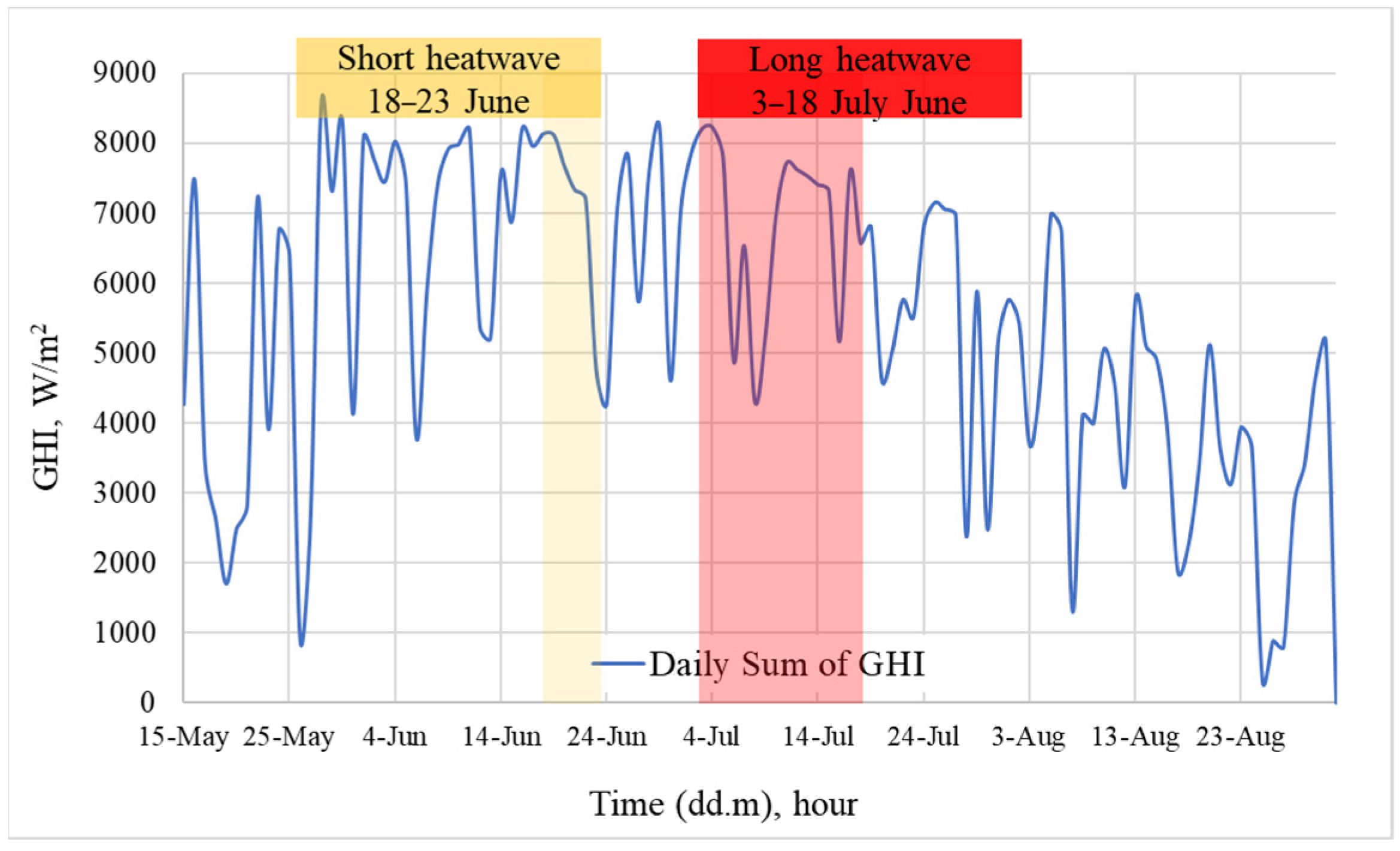
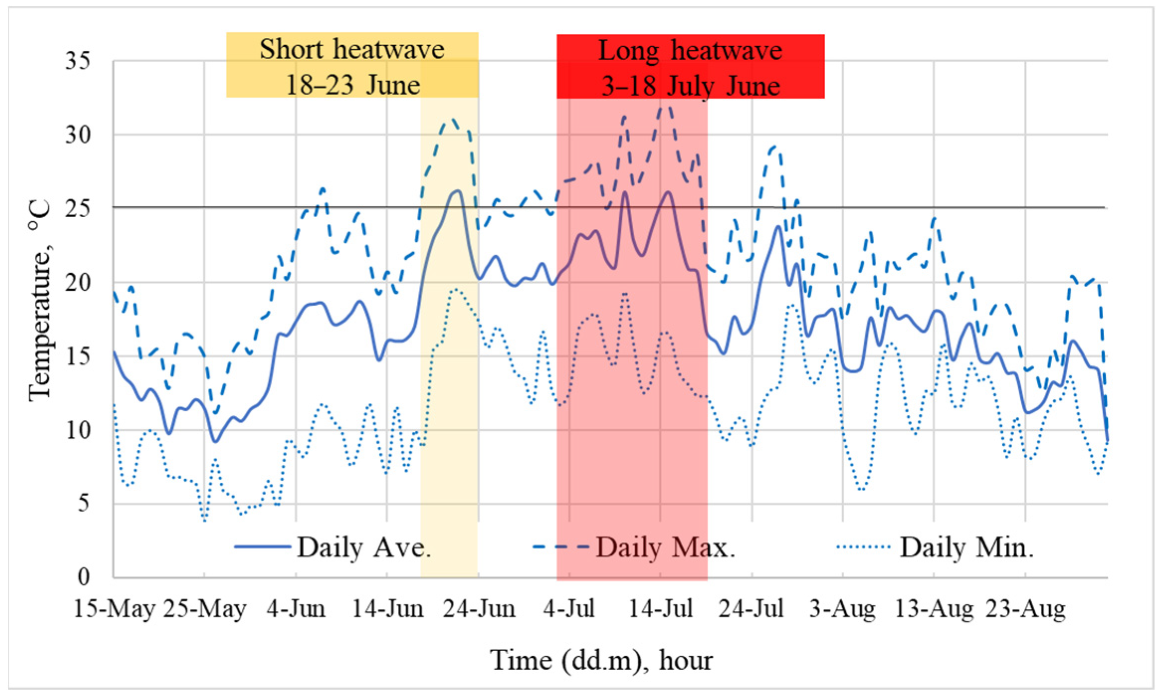
2.2. Outdoor Weather during the Hot Summer of 2021

Finland is a northern country in Europe, and its climate belongs to the Df category in the Köppen Geiger climate classification [25], indicating subarctic (or boreal) climate conditions. The southern coast of Finland, where the studied buildings are located, is classified as having a Dfb climate, which is cold, has no dry season, and has warm summers [25]. The summer of 2021 was one of Finland’s hottest summers in the last 30 years [19]. Figure 1 shows the outdoor daily average, maximum, and minimum temperatures, and Figure 2 shows the daily sum of GHI during the summer of 2021. The outdoor weather data was collected from the Helsinki Vantaa weather station and measured by the Finnish Meteorological Institute.

A hot day in Finland is defined as a day with a daily maximum temperature higher than 25 °C [26]. In this study, a heatwave was defined when there were more than 4 consecutive hot days. As Figure 1 shows, there were two heatwaves in the summer of 2021: a short one from 18–23 June, and a long one from 3–18 July. During the short heatwave, the outdoor temperature rose for a few days and then fell while the outdoor GHI was falling. During the long heatwave, there were fluctuations in the outdoor temperature and the outdoor GHI. However, the general trend in the outdoor temperature was sloping up during the long heatwave.

2.3. Statistical Analysis Methods

In this study, to explore the correlation between daily average indoor temperature and daily average outdoor temperature, as well as the daily sum of outdoor global horizontal irradiance (GHI), the Spearman’s rank-order correlation method was used [27]. This is a nonparametric measure of statistical dependence between two variables. It assesses how well the relationship between two variables can be described using a monotonic function. This type of correlation is appropriate when the assumptions for Pearson’s correlation are not met, particularly when the data is not normally distributed. In this study, it was used because the distribution of daily average outdoor temperature and GHI was not normal. Spearman’s correlation coefficient “ρ” was calculated for each apartment. This can have a value from −1 to 1, where −1 indicates a perfect negative monotonic correlation, 1 indicates a perfect positive monotonic correlation, and 0 indicates no monotonic correlation [27]. The Python module Statistical Functions (scipy.stats) was used for carrying out the correlation analyses.

The moving averages for the daily average outdoor temperature, as well as the daily sum of GHI, were calculated. For each day, the outdoor average temperature and the daily sum of GHI were calculated. This was achieved by summing all the temperature readings for the day and dividing by the number of readings, and summing all the GHI readings for the day. To calculate the moving average, a window size (e.g., 3 days, 5 days, etc.) was chosen. For each day in the time series, the average temperature for that day and the previous days, up to the window size, was calculated. For example, with a 3-day window, the moving average on the fourth day would be the average of the daily averages from the second, third, and fourth days.

To calculate the magnitude of the effect of each outdoor weather parameter (outdoor daily average temperature and the daily sum of GHI) on the daily average indoor temperature, multiple linear regression was used. Multiple linear regression (Equation (1)) is a statistical technique used to analyze the relationship between a dependent variable (indoor daily average temperature) and two or more independent variables (outdoor daily average temperature and the daily sum of GHI) [28]. It extends simple linear regression, which deals with one predictor variable, to account for multiple independent variables. The model estimates coefficients for each independent variable, allowing the prediction of the value of the dependent variable. The general form of the multiple linear regression model can be expressed as:

Y = β₀ + β₁X₁ + β₂X₂ + … + β_nX_n + ϵ

(1)

where:

Y represents the dependent variable.

X₁, X₂, …, X_n are the independent variables.

β₀ is the y-intercept (constant term).

β₁, β₂, …, β_n are the coefficients of the independent variables which represent the change in the dependent variable for one unit of change in the respective independent variable, holding other variables constant.

ϵ is the error term, representing the difference between observed and predicted values.

This model is commonly used in various fields to understand how multiple factors affect an outcome [28]. In this study, the Python module Statsmodels was used for the linear model. The coefficients corresponding to the outdoor daily average temperature and the daily sum of GHI were investigated to show the magnitude of their effects on indoor daily average temperature.

To understand how well the regression model fits, the R-squared value (Equation (2)), the coefficient of multiple determination, was used. This statistic measures the proportion of variance in the dependent variable that is predictable from the independent variables. It ranges from 0 to 1, with higher values indicating a better fit of the model to the data [29].

$${\mathrm{R}}^2=1-\frac{\mathrm{T}\mathrm{o}\mathrm{t}\mathrm{a}\mathrm{l}\hspace{0.17em}\mathrm{S}\mathrm{u}\mathrm{m}\hspace{0.17em}\mathrm{o}\mathrm{f}\hspace{0.17em}\mathrm{S}\mathrm{q}\mathrm{u}\mathrm{a}\mathrm{r}\mathrm{e}\mathrm{s}\left(\mathrm{S}\mathrm{S}\mathrm{T}\right)}{\mathrm{S}\mathrm{u}\mathrm{m}\hspace{0.17em}\mathrm{o}\mathrm{f}\hspace{0.17em}\mathrm{S}\mathrm{q}\mathrm{u}\mathrm{a}\mathrm{r}\mathrm{e}\mathrm{s}\hspace{0.17em}\mathrm{o}\mathrm{f}\hspace{0.17em}\mathrm{R}\mathrm{e}\mathrm{s}\mathrm{i}\mathrm{d}\mathrm{u}\mathrm{a}\mathrm{l}\mathrm{s}\left(\mathrm{S}\mathrm{S}\mathrm{R}\right)}$$

(2)

The sum of Squares of Residuals (SSR), also known as the sum of squared errors of prediction, is the sum of the squares of the differences between the observed values and the predicted values.

The total Sum of Squares (SST) represents the total variance in the dependent variable. It is the sum of the squares of the differences between the observed values and their means.

It is worth mentioning that the outdoor daily average temperatures and the daily sum of GHI were correlated (r = 0.63). Therefore, the multicollinearity was checked by calculating the Variance Inflation Factor (VIF) for each of them. VIF calculation (Equation (3)) is based on each design variable as a response variable and measuring its coefficient of determination R². When the VIF value is over five, it is an indication that the associated regression coefficients are poorly estimated because of multicollinearity [30]. The VIF for the outdoor daily average temperature and the daily sum of GHI was 1.64, indicating a low level of multicollinearity. Thus, the correlation between the outdoor daily average temperature and the daily sum of GHI appeared not to be a concern for the regression analysis.

$$\mathrm{V}\mathrm{I}\mathrm{F}=\frac{1}{1-{\mathrm{R}}^2}$$

(3)

Further, we used a normalization technique to scale the parameters. Normalization is essential because it standardizes the scale of variables, enabling fair comparisons, preventing algorithm sensitivity to variable scales, aiding optimization convergence, improving interpretability, handling outliers, enhancing data visualization, and ultimately leading to better model performance in data analysis. Z-score normalization is a technique used to transform data into a standard scale with a mean of 0 and a standard deviation of 1 [31]. It is particularly useful when dealing with variables that have different units or scales. To standardize a variable using this method, the mean of the variable is subtracted from each data point and then divided by the standard deviation [31].

2.4. Overheating Assessment Criteria

In Finland, two sets of criteria address the issue of overheating. These include requirements from the Ministry of the Environment for new buildings, and requirements from the Ministry of Social Affairs and Health of Finland for existing buildings. According to the Ministry of the Environment of Finland [32], 27 °C is the design temperature for the summertime. Moreover, new apartment buildings in the design phase must prove that there are no more than 150 Kh degree hours above 27 °C in living spaces during the summer months (June–August) based on the simulation results using Test Reference Year (TRY) 2012 [33]. The same requirement applies to all apartments, whether they have mechanical cooling or various ventilation systems (natural or mechanical). Complying with this threshold is possible through various passive and active solutions, except for openable windows [32]. This means that the openable windows cannot be used in the simulations for getting the construction permit.

In existing residential buildings, the maximum indoor temperature in the living spaces should not exceed 32 °C. This value in the spaces for elderly people is 30 °C. This is mandated by the Ministry of Social Affairs and Health [34]. With these three established thresholds, we were prompted to extend our calculations beyond the initial range and consider temperature levels ranging from 27 °C to 35 °C. Therefore, to see the temporal effects of heatwaves, we calculated the consecutive days in which the temperatures were always (24 h) higher than 27, 28, 29, …, 35 °C.

3. Results

3.1. Temporal Analysis of Overheating Risks

Table 1. Temporal analysis of overheating in the studied apartments.

Percentage (%) of Apartments with
		1 Day	2 Days	3 Days	4 Days	5 Days	6 Days	7 Days
Hourly temperature higher than	27 °C	84.8	77.9	69.8	61.0	55.1	50.0	46.8
	28 °C	59.6	48.8	40.2	32.7	26.2	21.5	19.2
	29 °C	28.1	20.9	15.8	11.8	8.8	6.2	5.3
	30 °C	8.3	5.5	3.9	2.8	1.9	1.5	1.2
	31 °C	1.8	1.3	0.9	0.6	0.3	0.2	0.2
	32 °C	0.4	0.3	0.2	0.2	0.1	0.1	0.1
	33 °C	0.1	0.1	0.1	0.1	0.1	0.0	0.0
	34 °C	0.05	0.05	0.05	0.05	0.05	0.0	0.0
	35 °C	0.05	0.03	0.03	0.03	0.03	0.0	0.0

shows the percentage of apartments with hourly temperatures consistently higher than the thresholds (27–35 °C) for 1 to 7 days during the summer of 2021 (mid-May to the end of August). It shows that almost half of the apartments experienced 7 days higher than 27 °C, indicating prolonged exposure to high indoor temperatures in a significant portion of the apartments. Considering 27 °C as the upper range of thermal comfort based on EN standards [35], this indicates an extended period of thermal discomfort.

While in our previous study, it was shown that around one-third of the apartments experienced summertime maximum temperatures higher than 30 °C for at least one hour [19], results revealed that the indoor temperature in more than 8% of the apartments (around 500 units) exceeded 30 °C (the health limit for elderly people) for 1 day, in almost 3% of apartments for 4 days, and in 1% of apartments for 7 days. Although these percentages are relatively low, they show high health risks for elderly people because of prolonged overheating time in apartments. The percentage of apartments with temperatures above 32 °C for 1 to 7 days was below 1%.

3.2. Indoor Temperature Dynamics Based on Outdoor Weather Conditions

In this section, we analyzed the indoor daily average temperatures in the apartments based on the outdoor daily average temperature and the outdoor daily sum of GHI as the two main parameters of outdoor weather conditions. Further, the effects of the number of hot days in the week on indoor temperatures were investigated in this study.

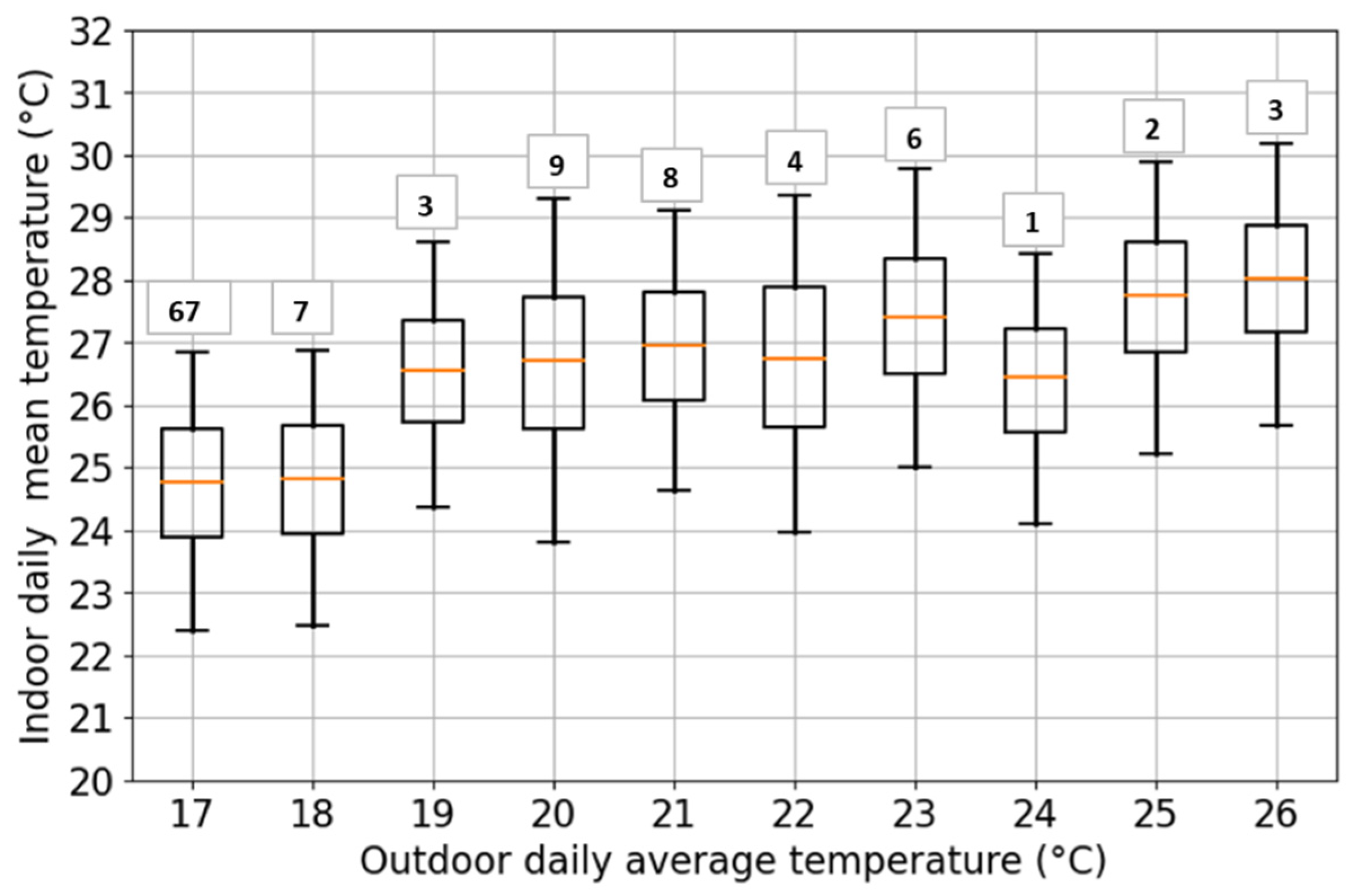
3.2.1. Indoor Temperature Variations Based on the Outdoor Average Temperature

Figure 3 illustrates how indoor daily average temperatures changed in response to varying outdoor daily average temperatures (for 5 to 95% of the apartments). These results were calculated for the period of the 4th of June to the 17th of August 2021, when the outdoor daily average temperature was higher than 17 °C. The reason we chose this period was that the focus of this study was on high indoor temperatures. The graph highlights two distinct outdoor daily average temperature changes, namely 18 °C to 19 °C and 22 °C to 23 °C, which corresponded to noticeable shifts in the indoor daily average temperatures, with the average of indoor daily average temperatures increasing to above 27 °C. Despite these clear shifts in indoor daily temperatures, it is challenging to label any specific outdoor average temperature as critical, due to the considerable variations in indoor daily temperatures. It is worth mentioning that the outdoor daily average temperature of 24 °C happened on just one day at the end of July, after some relatively cool days (See Figure 1). This could explain why indoor temperatures were low on that day.

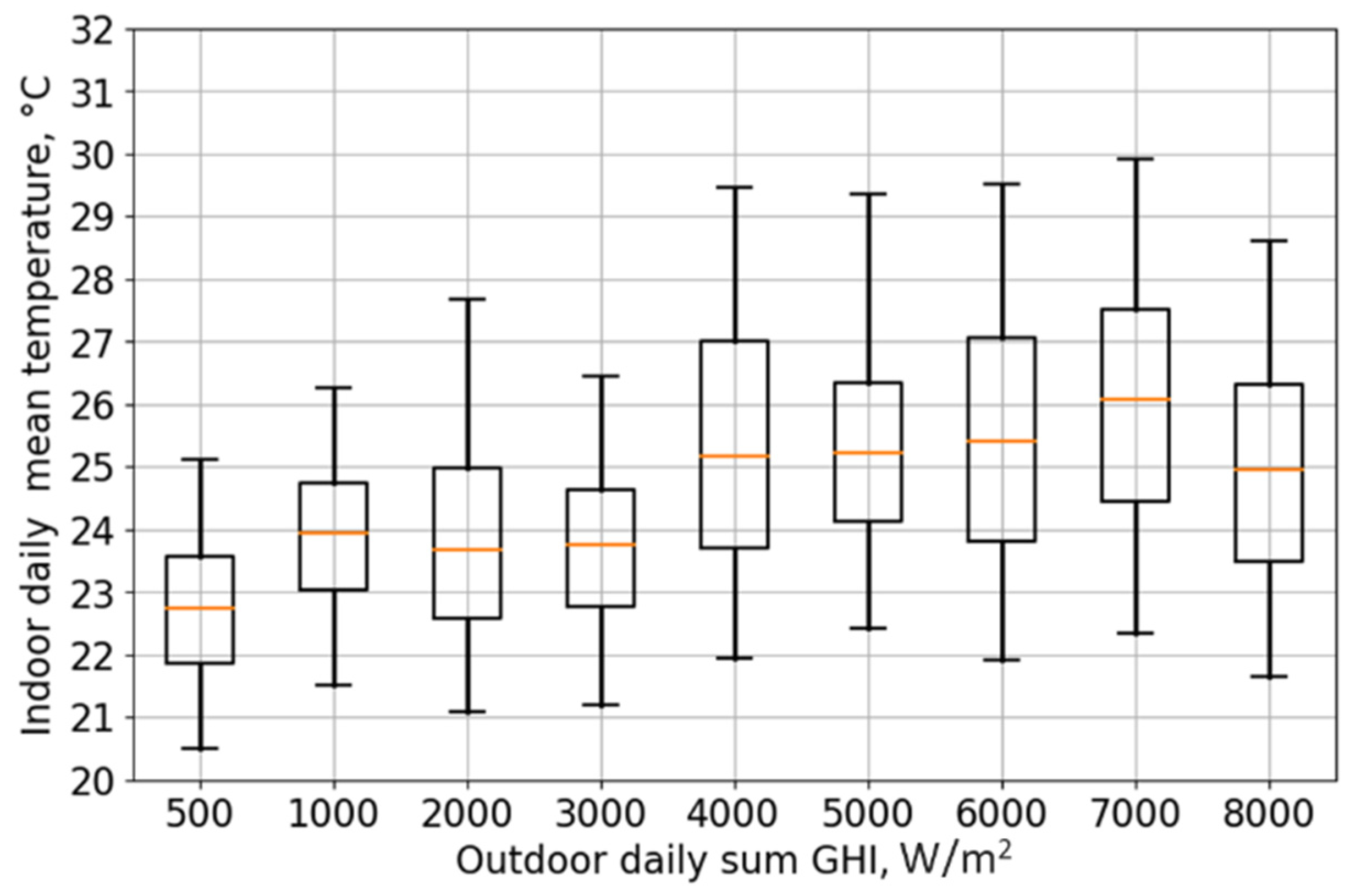
3.2.2. Indoor Temperature Variations Based on the Sum of GHI

Figure 4 depicts how indoor daily average temperatures correlated in response to varying daily sums of GHI for the whole summer of 2021. The graph highlights three distinct outdoor daily sums of GHI points, namely 500 to 1000 W/m², 3000 to 4000 W/m², and 6000 to 7000 W/m², which corresponded to notable shifts in the indoor daily average temperatures.

Although there were considerable variations in indoor temperatures, these three numbers can be labeled as defining limits for the sum of GHI. It is worth mentioning that the outdoor daily sum of GHI of 8000 W/m² happened during the cool days of early summer (see Figure 2). This could explain why indoor temperatures were low despite a GHI of 8000 W/m². Moreover, this shows that even with high outdoor solar radiation, there can be low outdoor temperature levels and therefore, low indoor temperature levels. Thus, the association between solar radiation and indoor temperature seems to be not straightforward.

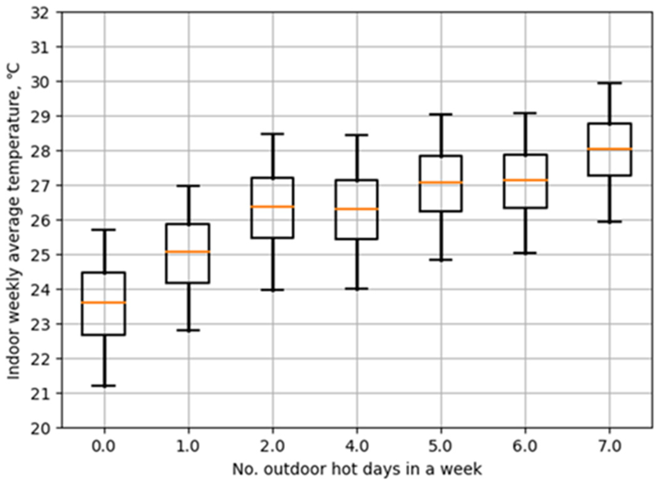
3.2.3. Indoor Temperature Variations Based on Weekly Number of Hot Days

Figure 5 shows how indoor weekly average temperatures change in response to the number of hot days in the week (consecutive or not). The graph highlights three distinct numbers of hot days, namely no hot day to 1, 4 to 5, and 6 to 7 days, which correspond to notable shifts in the indoor weekly average temperatures. It indicates that with more than 5 hot days in a week, the average indoor weekly temperature tended to be higher than 27 °C, while 7 hot days would cause the average indoor weekly temperature to be higher than 28 °C. In the hottest apartments (exhibiting the maximum weekly average temperature), the average indoor weekly temperature reached 30 °C. Further, if there were no hot days in the week, the indoor weekly temperature was relatively low, with even the hottest apartments exhibiting temperatures lower than 26 °C.

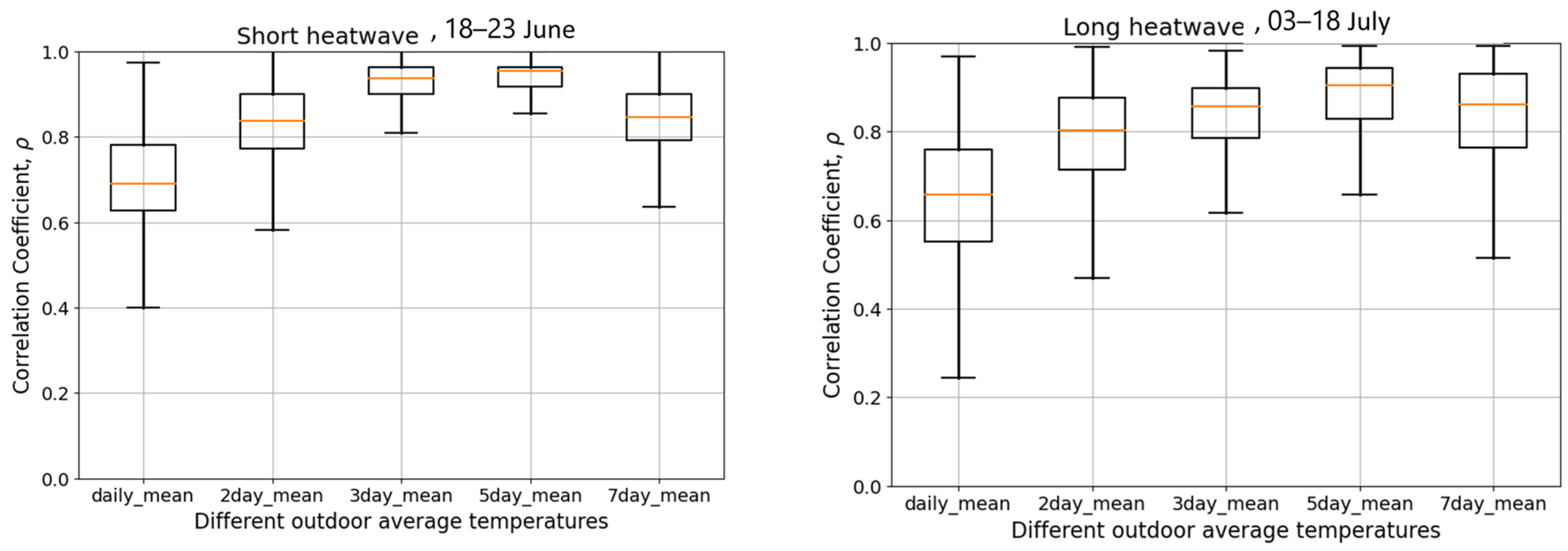
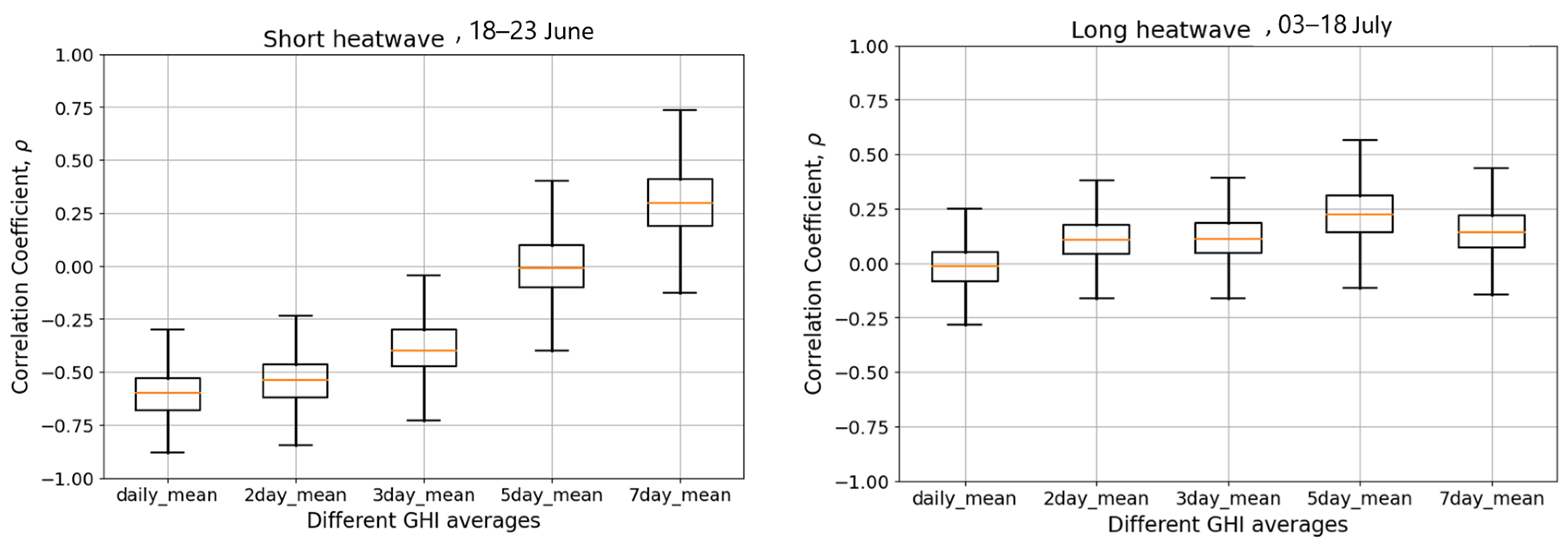
3.3. Correlation between Indoor Temperature and Outdoor Weather Conditions

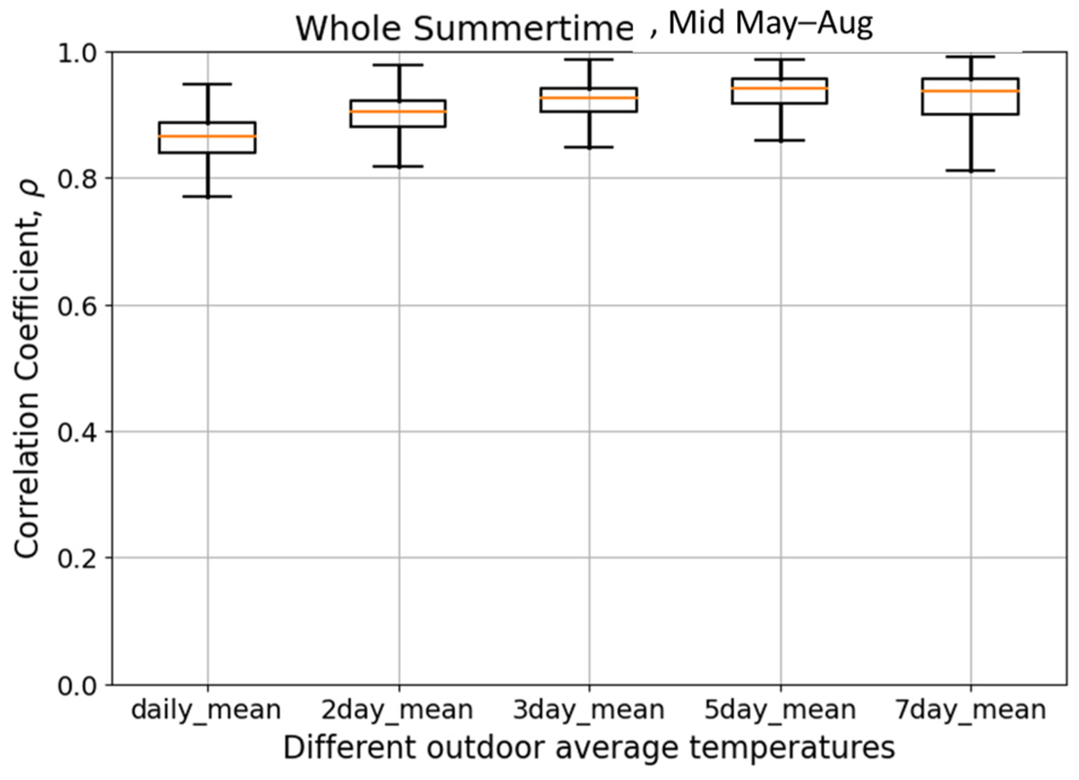
3.3.1. Outdoor Temperature

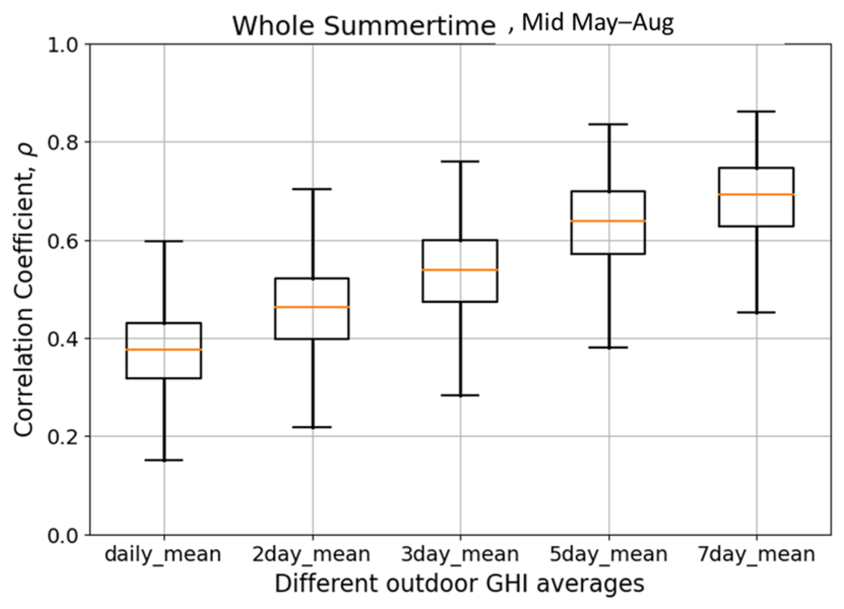
To examine how outdoor temperature influences indoor temperature levels, we conducted a correlation analysis between outdoor daily temperatures and the daily average indoor temperature. This analysis was performed using different outdoor moving averages, specifically 2, 3, 5, and 7-day averages, to investigate the effects of the building’s thermal mass and weather history. Furthermore, these calculations were carried out for the entire summer period (mid-May to the end of August 2021), as well as for the short and long heatwaves, allowing us to explore how the duration of heatwaves impacts the relationship between indoor and outdoor temperature.

Figure 6 and Figure 7 show Spearman’s correlation coefficient “ρ” value results for the whole summer period, and the short and long heatwaves, respectively. As can be seen, there was a strong correlation between indoor daily average temperature and different outdoor average temperatures during the whole summertime, with the correlation coefficient “ρ” value remaining higher than 0.75. The correlation coefficient “ρ” values for daily, 2-day, and 3-day averages were lower than the whole summer for both heatwaves. Further, the correlation coefficient “ρ” values for the long heatwave were lower than the short heatwave. As the duration of outdoor temperature averaging increased, so did the correlation coefficient during the whole summer and both heatwaves. The highest correlation was observed with the 5-day moving average of outdoor temperatures, and then it decreased.

The highest correlation with the 5-day moving average of outdoor temperatures during the whole summer, as well as the short and long heatwaves, suggests that outdoor temperature patterns over 5 days have a more significant influence on indoor temperature levels, potentially reflecting the lag or delayed effects of outdoor temperature changes and the building’s thermal mass on indoor conditions.

3.3.2. GHI

To examine how outdoor solar radiation affects indoor temperature levels, we conducted a correlation analysis. This analysis focused on examining the relationship between the daily sum of GHI and the daily average indoor temperatures. Additionally, we expanded our analysis to include various outdoor moving averages of the daily GHI, including 2, 3, 5, and 7-day averages. Furthermore, these calculations were carried out for the entire summer period, as well as for the short and long heatwaves, allowing us to explore how the duration of heatwaves impacts the relationship between indoor temperature and solar radiation.

Figure 8 shows Spearman’s correlation coefficient “ρ” value results of this correlation analysis for the whole summer period. As can be seen, there was a relatively weak correlation between indoor daily average temperature and the daily sum of GHI for 2 to 3-day moving averages, with the median of Spearman’s correlation coefficient “ρ” values being lower than 0.7. As the duration of outdoor GHI averaging increased, so did the correlation coefficient. The highest correlation was observed with the 7-day moving average of outdoor GHI (the median around 0.75). This suggests that outdoor GHI patterns over 7 days have a more significant influence on indoor temperature levels, potentially reflecting the cumulative effect of the outdoor GHI changes on indoor conditions. It is worth mentioning that the Spearman’s correlation coefficient “ρ” values of this correlation were, in general, lower than the correlation between indoor and outdoor temperature levels.

Figure 9 shows Spearman’s correlation coefficient “ρ” values for the short and long heatwave periods, respectively. The relationship between indoor temperature and solar radiation during heatwaves was more complex compared to the relationship between indoor and outdoor temperatures.

During the short heatwave, an inverse correlation was observed between the average indoor temperature and the daily sum of GHI, as well as its 2 and 3-day moving averages. Upon considering Figure 2, it becomes apparent that during this short heatwave period, while outdoor temperatures were on the rise, the daily sum of GHI was decreasing. However, as the duration of averaging increased, the correlation coefficient became positive and larger. The highest median value was around 0.3, between the indoor daily average temperature and the 7-day moving average of the daily sum of GHI. During the long heatwave, the correlation was weak because the thermal mass was already warmed up. The highest median of the coefficients was around 0.25, between the indoor daily average temperature and the 5-day moving average of the daily sum of GHI.

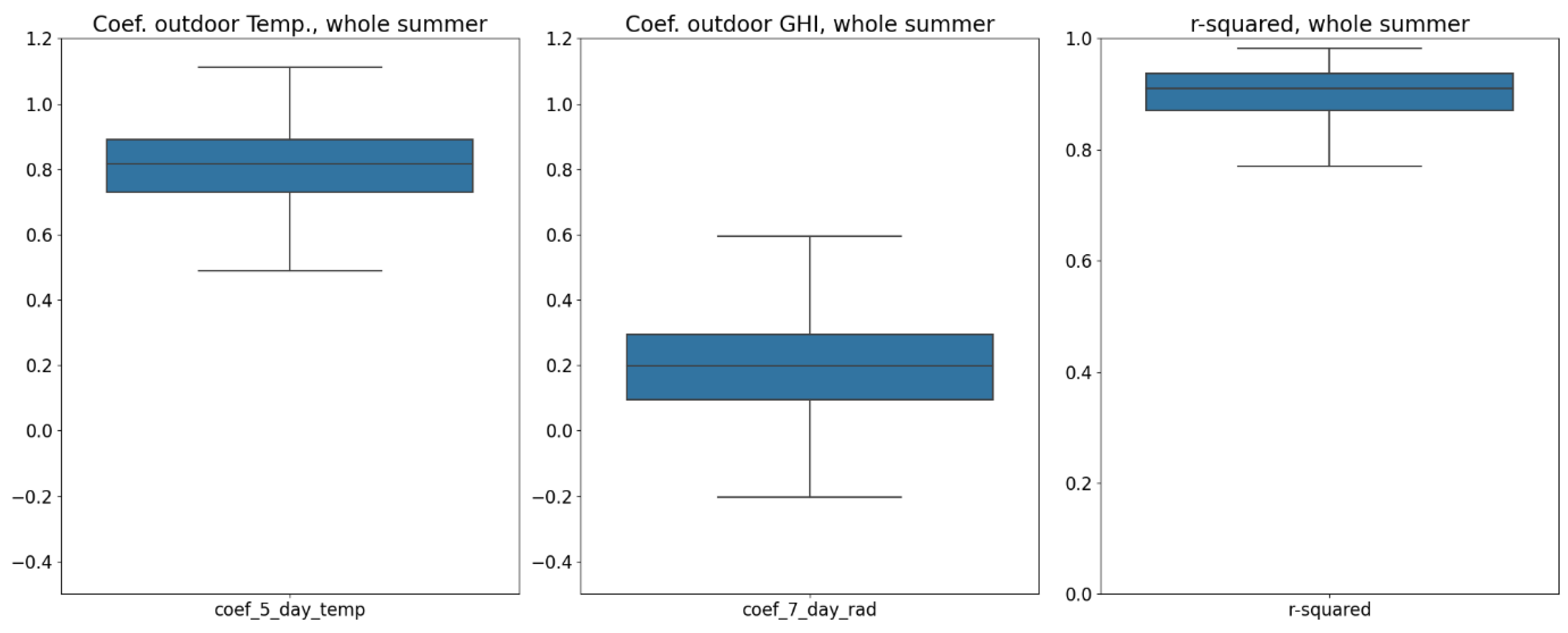
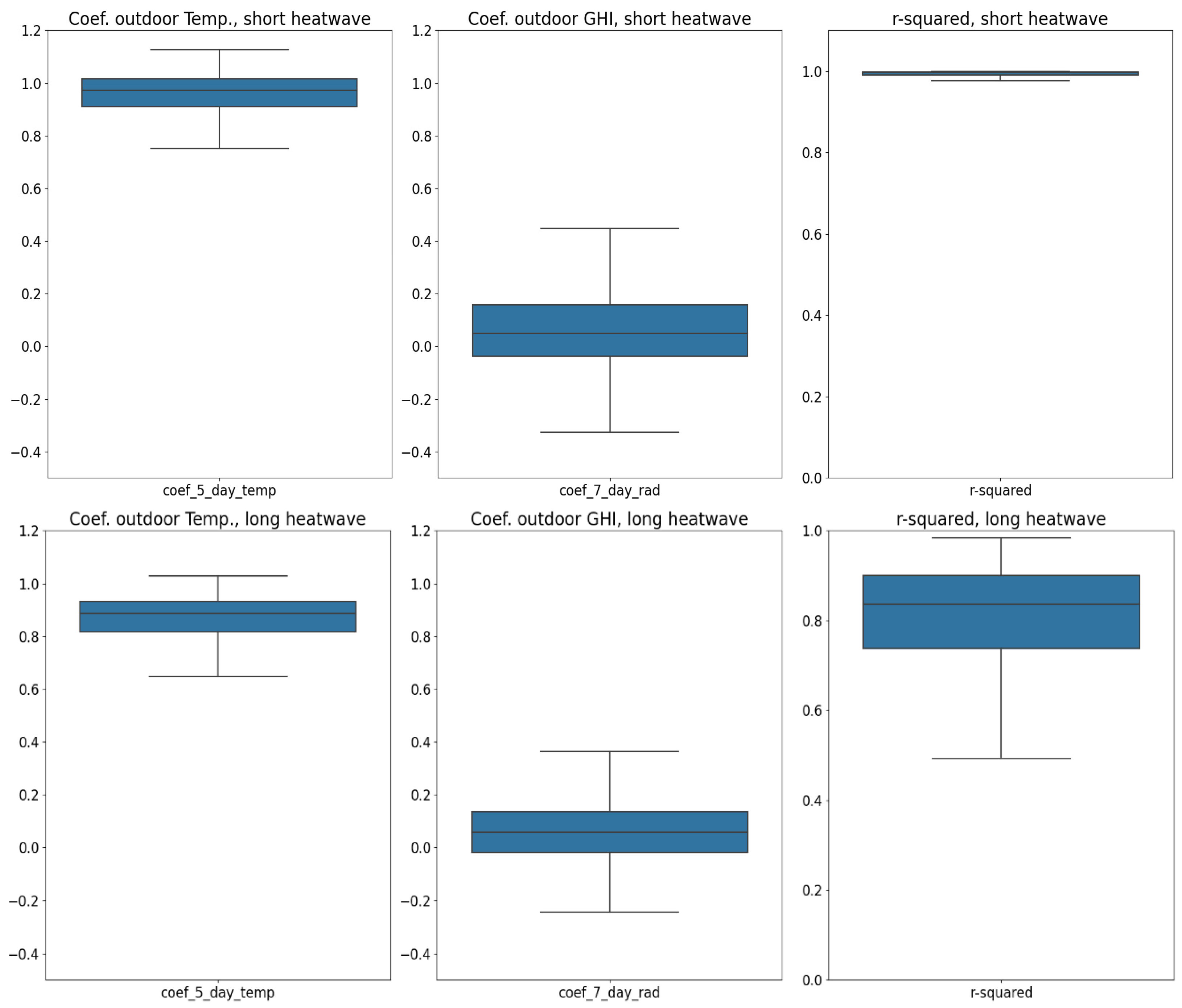
3.4. Multiple Linear Regression between the Indoor Temperature and Outdoor Weather Conditions

To investigate the extent of the influence of outdoor temperature and solar radiation on indoor temperature levels, we performed multiple linear regression analyses involving the most strongly correlated parameters. As the results of the previous section showed, there were strong correlations between the indoor daily average temperature and the outdoor 5-day moving average temperature, and the 7-day moving average of the daily sum of GHI. It is worth mentioning that the 7-day moving average of the daily sum of GHI was used for the whole summer and both heatwaves since the correlation was strong during the whole summer. Therefore, these parameters were normalized with the Z-score method (see Section 2.2), and then the multiple linear regression was conducted between these parameters for each of the studied apartments.

Figure 10 shows the variation of coefficients of each parameter, as well as r-squared values for all the apartments, during the whole summer. The r-squared range was between 0.77 to 0.97, with an average of 0.92. This indicates a strong linear relationship between the variables. The coefficient of outdoor temperature varied across different apartments with values between 0.5 and 1.1 and a median of 0.8, and the coefficient of GHI varied between −0.2 and 0.6 with a median of 0.2, showing that the effect of the outdoor 5-day moving average temperature on the indoor average temperature was more notable than the effect of the 7-day moving average GHI (0.8 > 0.2).

Figure 11 shows the results of the multiple linear regression during the long and short heatwaves. The high r-squared range with averages of 0.99 and 0.85 for the short and long heatwaves, respectively, shows a strong linear relationship between the variables during heatwaves. This suggests that the outdoor 5-day moving average temperature and outdoor 7-day moving average GHI used in the regression model were highly effective at explaining the variation in the indoor daily average temperature under heatwave conditions. The coefficient of outdoor temperature was higher (average ≅ 1) for the short heatwave in comparison with the whole summer and the long heatwave. This observation implies that changes in outdoor temperature have a more significant impact on indoor temperature levels during short heatwave periods, possibly due to the rapid and extreme temperature fluctuations characteristic of such events.

Further, the coefficient of outdoor GHI was lower (average ≅ 0.1) for both the short and long heatwaves compared to the whole summertime. This finding suggests that the influence of GHI on indoor temperature levels is diminished during heatwave conditions, possibly due to factors such as reduced solar radiation caused by increased cloud cover.

These significant variations in coefficients between the short and long heatwaves, as well as between heatwaves and the entire summer season, highlight the complex and dynamic nature of these relationships under different environmental conditions.

4. Discussion

This study provides insights into the temporal analysis of overheating risks in apartments and the influence of outdoor weather conditions on indoor temperatures during hot summers and associated heatwaves. Nevertheless, it is important to acknowledge several limitations in this study that should be considered when interpreting the findings. The extensive dataset of hourly indoor temperatures in over 6000 apartments has constrained access to numerous intervening factors, including aspects such as building envelope characteristics, occupant behavior, apartment layout and orientation, window-to-wall ratios, and more. Many of these can affect the indoor temperature levels more or less than the analysed parameters of outdoor temperature and solar radiation.

However, it is essential to clarify that the primary objective of this study was not to identify all potentially effective parameters influencing indoor temperature levels or to pinpoint the most effective ones. Instead, our focus was on assessing the impact of hot summer conditions and their corresponding outdoor factors on indoor temperatures within residential buildings. We aimed to estimate the extent of health and comfort challenges arising from climate change and its associated hot summers. Future research should focus on examining this relationship considering building design and characteristics, providing more precise guidance for designers to select suitable heat mitigation strategies.

Moreover, while the focus of this study was primarily on indoor temperature dynamics, it is worth mentioning that relative humidity plays a significant role in shaping occupants’ perception of thermal comfort. The exclusion of relative humidity from our analysis may limit the comprehensiveness of our findings, as it represents an essential aspect of the indoor thermal environment. Relative humidity influences the body’s ability to regulate heat through evaporation, impacting thermal comfort even at a constant temperature. Thus, despite the high indoor overheating shown in the results, thermal comfort conditions in residential buildings during heatwaves should be analysed further.

The study’s findings regarding prolonged exposure to high indoor temperatures, especially for elderly residents, highlight the potential health risks associated with hot summers and heatwaves in residential buildings, where nearly half of the apartments experienced temperatures exceeding 27 °C for seven consecutive days. Notably, a recent study on elderly people’s thermal comfort in warm conditions indicated that the elderly’s neutral and preferred temperatures are 26 °C and 26.5 °C, respectively [36]. This discrepancy highlights the significance of these findings, showing high risks of thermal discomfort.

A study on mortality rate and heatwaves showed that during heatwave days, when the outdoor daily average temperature in Southern Finland was 22.9 °C, the overall mortality rate increased by 9.9% [13]. Another recent study in Finland showed that daily high temperature increases mortality by an average of 2.7% with a one degree increase from the reference point of 18.8 °C [37]. Therefore, the outdoor temperature rise to 22–23 °C would cause around a 10% increase in premature mortality of elderly persons above 65 years old. This aligns with our results, which show that a slight shift in outdoor daily average temperature, from 22 °C to 23 °C, can cause indoor daily average temperatures to exceed 27 °C. These insights highlight the importance of taking action toward preventing indoor summertime overheating in cold climates with the rise of climate change in order to protect the well-being of occupants, and especially vulnerable populations.

Moreover, understanding the correlation between outdoor weather conditions and indoor temperatures provides occupants with valuable insights, enabling them to anticipate indoor temperature trends based on weather forecasts and early warnings of heat waves. Consequently, occupants can proactively prepare for potential indoor overheating by taking suitable action, such as using night cooling strategies or personal cooling devices.

Further, the results of this study align with other studies focusing on the correlation between outdoor and indoor temperatures in residential buildings. They showed that the correlation varied in different seasons [20,23]. Different correlation results during the short and long heatwaves as well as whole summers show the complexity of the relationship between outdoor weather conditions and indoor temperature levels. This emphasizes the importance of considering extreme heat events in building design and operation. It can help designers develop more suitable strategies to reduce energy consumption for cooling and heating, potentially leading to cost savings and reduced carbon emissions. Additionally, the study’s insights into revising policies and guidelines consider the increasing frequency of heat events in cold climates.

The findings of this study indicate that during heatwaves, indoor temperatures are more influenced by outdoor temperatures than by solar radiation. This was shown in another study as well [20]. This can be attributed to the mechanical ventilation systems, which supply warm air from the outside into apartments, and the highly insulated and airtight envelope that traps heat inside. Although windows contribute to indoor overheating with solar heat gains, the impact of the ventilation system is more pronounced, particularly on cloudy days when solar radiation is less intense. This emphasizes the significant role that building design and ventilation play in regulating indoor temperatures during extreme weather conditions.

5. Conclusions

In this study, we investigated the impact of outdoor conditions on indoor temperatures during hot summers and associated heatwaves, using a large dataset of over 6000 apartments in the cold climate of Finland.

Based on the results, high summertime overheating levels and long overheating periods are expected under climate change in the apartments of cold climates. Nearly half of the studied apartments experienced indoor temperatures surpassing 27 °C (upper limit of thermal comfort, and 1 °C higher than the neutral temperature for elderly people) for more than 7 continuous days in the summer of 2021 in Finland. With the current design of the apartments in Finland, even an outdoor average daily temperature of 19 °C led to an indoor average daily temperature of over 27 °C, and 5 hot days in a week could lead to high indoor temperature levels.

Further, the results revealed a strong positive correlation between indoor average temperature and outdoor daily average temperatures during the summer; the correlation weakened during prolonged heatwaves. The highest correlation, between the indoor daily temperature and the 5-day moving average, signals a time lag between indoor and outdoor temperatures to reach their maximum values. This can provide occupants with an opportunity to take proactive measures to alleviate overheating.

Additionally, a strong positive correlation was observed between indoor average temperature and the 7-day moving average of the sum of GHI. However, during heatwaves, the correlation is not always positive. A high level of inverse correlations is revealed during the short and long heatwaves. This shows that if there is cloudiness, the indoor temperature is mainly affected by outdoor temperature.

The high r-squared values show the multiple linear regression between indoor daily average temperature, outdoor 5-day moving average temperature, and 7-day moving GHI fits well. There were notable variations in the magnitude of the effects of the outdoor temperature and outdoor solar radiation between short and long heatwaves, as well as between heatwaves and the entire summer season. This highlights the complex and dynamic nature of these relationships under different environmental conditions and emphasizes the importance of considering extreme heat events in the design and operation of buildings in cold climates.

References

1. Arsad, F.S.; Hod, R.; Ahmad, N.; Ismail, R.; Mohamed, N.; Baharom, M.; Osman, Y.; Radi, M.F.M.; Tangang, F. The Impact of Heatwaves on Mortality and Morbidity and the Associated Vulnerability Factors: A Systematic Review. Int. J. Environ. Res. Public. Health 2022, 19, 16356. [Google Scholar] [CrossRef] [PubMed]
2. Heino, M.; Kinnunen, P.; Anderson, W.; Ray, D.K.; Puma, M.J.; Varis, O.; Siebert, S.; Kummu, M. Increased probability of hot and dry weather extremes during the growing season threatens global crop yields. Sci. Rep. 2023, 13, 3583. [Google Scholar] [CrossRef] [PubMed]
3. Dunne, J.P.; Stouffer, R.J.; John, J.G. Reductions in labour capacity from heat stress under climate warming. Nat. Clim. Chang. 2013, 3, 563–566. [Google Scholar] [CrossRef]
4. Ruffault, J.; Curt, T.; Moron, V.; Trigo, R.M.; Mouillot, F.; Koutsias, N.; Pimont, F.; Martin-StPaul, N.; Barbero, R.; Dupuy, J.L.; et al. Increased likelihood of heat-induced large wildfires in the Mediterranean Basin. Sci. Rep. 2020, 10, 13790. [Google Scholar] [CrossRef] [PubMed]
5. Mulholland, E.; Feyen, L. Increased risk of extreme heat to European roads and railways with global warming. Clim. Risk Manag. 2021, 34, 100365. [Google Scholar] [CrossRef]
6. Klingelhöfer, D.; Braun, M.; Brüggmann, D.; Groneberg, D.A. Heatwaves: Does global research reflect the growing threat in the light of climate change? Glob. Health 2023, 19, 56. [Google Scholar] [CrossRef] [PubMed]
7. Masson-Delmotte, V.; Zhai, P.; Chen, Y.; Goldfarb, L.; Gomis, M.I.; Matthews, J.B.R.; Berger, S.; Huang, M.; Yelekçi, O.; Yu, R.; et al. Climate Change 2021: The Physical Science Basis. Contribution of Working Group I to the Sixth Assessment Report of the Intergovernmental Panel on Climate Change; IPCC: Paris, France, 2021; Available online: https://www.ipcc.ch (accessed on 5 March 2024).
8. Mikkonen, S.; Laine, M.; Mäkelä, H.M.; Gregow, H.; Tuomenvirta, H.; Lahtinen, M.; Laaksonen, A. Trends in the average temperature in Finland, 1847–2013. Stoch. Environ. Res. Risk Assess. 2015, 29, 1521–1529. [Google Scholar] [CrossRef]
9. Ebi, K.L.; Capon, A.; Berry, P.; Broderick, C.; de Dear, R.; Havenith, G.; Honda, Y.; Kovats, R.S.; Ma, W.; Malik, A.; et al. Hot weather and heat extremes: Health risks. Lancet 2021, 398, 698–708. [Google Scholar] [CrossRef] [PubMed]
10. Ballester, J.; Quijal-Zamorano, M.; Méndez Turrubiates, R.F.; Pegenaute, F.; Herrmann, F.R.; Robine, J.M.; Basagaña, X.; Tonne, C.; Antó, J.M.; Achebak, H. Heat-related mortality in Europe during the summer of 2022. Nat. Med. 2023, 29, 1857–1866. [Google Scholar] [CrossRef] [PubMed]
11. Masselot, P.; Mistry, M.; Vanoli, J.; Schneider, R.; Iungman, T.; Garcia-Leon, D.; Ciscar, J.C.; Feyen, L.; Orru, H.; Urban, A.; et al. Excess mortality attributed to heat and cold: A health impact assessment study in 854 cities in Europe. Lancet Planet. Health 2023, 7, e271–e281. [Google Scholar] [CrossRef] [PubMed]
12. Sohail, H.; Lanki, T.; Kollanus, V.; Tiittanen, P.; Schneider, A. Heat, heatwaves and cardiorespiratory hospital admissions in Helsinki, Finland. Int. J. Environ. Res. Public Health 2020, 17, 7892. [Google Scholar] [CrossRef] [PubMed]
13. Kollanus, V.; Tiittanen, P.; Lanki, T. Mortality risk related to heatwaves in Finland–Factors affecting vulnerability. Environ. Res. 2021, 201, 111503. [Google Scholar] [CrossRef] [PubMed]
14. Astone, R.; Vaalavuo, M. Climate Change and Health: Consequences of High Temperatures among Vulnerable Groups in Finland. Int. J. Soc. Determ. Health Health Serv. 2022, 53, 94–111. [Google Scholar] [CrossRef] [PubMed]
15. Lomas, K.J.; Watson, S.; Allinson, D.; Fateh, A.; Beaumont, A.; Allen, J.; Foster, H.; Garrett, H. Dwelling and household characteristics’ influence on reported and measured summertime overheating: A glimpse of a mild climate in the 2050’s. Build Environ. 2021, 201, 107986. [Google Scholar] [CrossRef]
16. Gupta, R.; Gregg, M. Assessing the Magnitude and Likely Causes of Summertime Overheating in Modern Flats in UK. Energies 2020, 13, 5202. [Google Scholar] [CrossRef]
17. Maivel, M.; Kurnitski, J.; Kalamees, T. Field survey of overheating problems in Estonian apartment buildings. Archit. Sci. Rev. 2015, 58, 1–10. [Google Scholar] [CrossRef]
18. Kotol, M.; Rode, C.; Clausen, G.; Nielsen, T.R. Indoor environment in bedrooms in 79 Greenlandic households. Build. Environ. 2014, 81, 29–36. [Google Scholar] [CrossRef]
19. Farahani, A.V.; Kravchenko, I.; Jokisalo, J.; Korhonen, N.; Jylhä, K.; Kosonen, R. Overheating assessment for apartments during average and hot summers in the Nordic climate. Build. Res. Inf. 2023, 52, 273–291. [Google Scholar] [CrossRef]
20. Li, W.; Zhou, Z.; Wang, C.; Han, Y. Impact of outdoor microclimate on the performance of high-rise multi-family dwellings in cold areas and optimization of building passive design. Build. Environ. 2024, 248, 111038. [Google Scholar] [CrossRef]
21. Hou, Y.; Cao, B.; Zhu, Y.; Zhang, H.; Yang, L.; Duanmu, L.; Lian, Z.; Zhang, Y.; Zhai, Y.; Wang, Z.; et al. Temporal and spatial heterogeneity of indoor and outdoor temperatures and their relationship with thermal sensation from a global perspective. Environ. Int. 2023, 179, 108174. [Google Scholar] [CrossRef] [PubMed]
22. Zuurbier, M.; van Loenhout, J.A.F.; le Grand, A.; Greven, F.; Duijm, F.; Hoek, G. Street temperature and building characteristics as determinants of indoor heat exposure. Sci. Total Environ. 2021, 766, 144376. [Google Scholar] [CrossRef] [PubMed]
23. Nguyen, J.L.; Dockery, D.W. Daily indoor-to-outdoor temperature and humidity relationships: A sample across seasons and diverse climatic regions. Int. J. Biometeorol. 2016, 60, 221–229. [Google Scholar] [CrossRef] [PubMed]
24. Nguyen, J.L.; Schwartz, J.; Dockery, D.W. The relationship between indoor and outdoor temperature, apparent temperature, relative humidity, and absolute humidity. Indoor Air 2014, 24, 103–112. [Google Scholar] [CrossRef] [PubMed]
25. Peel, M.C.; Finlayson, B.L.; McMahon, T.A. Updated world map of the Köppen-Geiger climate classification. Hydrol. Earth Syst. Sci. 2007, 11, 1633–1644. [Google Scholar] [CrossRef]
26. FMI. Record-Breaking Temperatures in May. FMI Press Release Archive. 2018. Available online: https://en.ilmatieteenlaitos.fi/press-release/539036550 (accessed on 17 February 2021).
27. Corder, G.W.; Foreman, D.I. Nonparametric Statistics for Non-Statisticians: A Step-by-Step Approach; John Wiley & Sons, Inc.: Hoboken, NJ, USA, 2009. [Google Scholar]
28. Hair, J.F. Multivariate Data Analysis; Kennesaw State University: Kennesaw, GA, USA, 2009. [Google Scholar]
29. Lewis-Beck, M.S.; Skalaban, A. The R-Squared: Some Straight Talk. Political Anal. 1990, 2, 153–171. [Google Scholar] [CrossRef]
30. Sheather, S.J. A Modern Approach to Regression with R; Springer Science & Business Media: Berlin/Heidelberg, Germany, 2009; pp. 4–28. [Google Scholar]
31. Pedregosa, F.; Varoquaux, G.; Gramfort, A.; Michel, V.; Thirion, B.; Grisel, O.; Blondel, M.; Prettenhofer, P.; Weiss, R.; Dubourg, V.; et al. Scikit-learn: Machine Learning in Python. J. Mach. Learn. Res. 2011, 12, 2825–2830. [Google Scholar]
32. Decree (1010/2017) of the Ministry of the Environment, Indoor Climate and Ventilation of New Buildings. 2017, pp. 1–16. Available online: https://ym.fi/en/the-national-building-code-of-finland (accessed on 5 March 2024).
33. Kalamees, T.; Jylhä, K.; Tietäväinen, H.; Jokisalo, J.; Ilomets, S.; Hyvönen, R.; Saku, S. Development of weighting factors for climate variables for selecting the energy reference year according to the EN ISO 15927-4 standard. Energy Build. 2012, 47, 53–60. [Google Scholar] [CrossRef]
34. Ministry of Social Affairs and Health. Decree of the Ministry of Social Affairs and Health on Health-related Conditions of Housing and Other Residential Buildings and Qualification Requirements for Third-party Experts, 545/2015. 2015. Available online: https://www.finlex.fi/en/laki/kaannokset/2015/en20150545 (accessed on 5 March 2024).
35. Standard SFS-EN 16798-1; Part 1: Indoor Environmental Input Parameters for Design and Assessment of Energy Performance of Buildings Addressing Indoor air Quality, Thermal Environment, Lighting and Acoustics. Finnish Standards Association SFS: Helsinki, Finland, 2019. Available online: https://www.ds.dk (accessed on 5 March 2024).
36. Chen, M.; Farahani, A.V.; Kilpeläinen, S.; Kosonen, R.; Younes, J.; Ghaddar, N.; Ghali, K.; Melikov, A.K. Thermal comfort chamber study of Nordic elderly people with local cooling devices in warm conditions. Build. Environ. 2023, 235, 21–24. [Google Scholar] [CrossRef]
37. Kosonen, R.; Kurnitski, J.; Jokisalo, J.; Kilpeläinen, S.; Farahani, A.V.; Ejaz, M.F.; Simson, R.; Kollanus, V.; Lanki, T.; Tiittanen, P.; et al. Ilmanvaihto- ja Jäähdytysjärjestelmien Resilienssi Lämpöaaltojen ja Hengitystieinfektioiden Suhteen: Uudis- ja Korjausrakennusten Teknisten Ratkaisujen Toiminta Muuttuvissa Olosuhteissa. 2023. Available online: https://julkaisut.valtioneuvosto.fi/handle/10024/165209 (accessed on 5 March 2024).
Figure 1. Outdoor daily temperatures during the summer of 2021.
Buildings 14 01053 g001
Figure 2. Outdoor daily average GHI during the summer of 2021.
Buildings 14 01053 g002
Figure 3. Indoor daily average temperatures based on outdoor daily average temperatures. The number of days with certain outdoor daily average temperatures is written atop each box plot.
Buildings 14 01053 g003
Figure 4. Indoor daily average temperatures based on outdoor daily sum of GHI.
Buildings 14 01053 g004
Figure 5. Indoor weekly average temperatures based on the number of hot days in the week.
Buildings 14 01053 g005
Figure 6. Spearman’s Correlation coefficients between indoor daily average temperatures and different outdoor average temperatures in all the apartments during the whole summer period.
Buildings 14 01053 g006
Figure 7. Spearman’s Correlation coefficients between indoor daily average temperatures and different outdoor average temperatures in all the apartments during the short and long heatwaves.
Buildings 14 01053 g007
Figure 8. Spearman’s Correlation coefficients between indoor daily average temperatures and different average GHI in all of the apartments during the whole summer period.
Buildings 14 01053 g008
Figure 9. Spearman’s Correlation coefficients between indoor daily average temperatures and different average GHI in all the apartments during the short and long heatwaves.
Buildings 14 01053 g009
Figure 10. The multiple linear regression between the indoor daily average temperature, the 7-day moving average GHI, and the outdoor 5-day sliding average temperature in all the apartments during the whole summer.
Buildings 14 01053 g010
Figure 11. The multiple linear regression between the indoor daily average temperature, the outdoor 7-day moving average GHI, and the outdoor 5-day moving average temperature in all the apartments during the short and long heatwaves.
Buildings 14 01053 g011