Article

The Use of Lidar and Artificial Intelligence Algorithms for Detection and Size Estimation of Potholes

1
Applied Research Associates Inc., Camp Hill, PA 17011, USA
2
Center for Smart, Sustainable & Resilient Infrastructure (CSSRI), Department of Civil & Architectural Engineering & Construction Management, University of Cincinnati, Cincinnati, OH 45221, USA
*
Author to whom correspondence should be addressed.
Buildings 2024, 14(4), 1078; https://doi.org/10.3390/buildings14041078
Submission received: 28 December 2023 / Revised: 22 March 2024 / Accepted: 1 April 2024 / Published: 12 April 2024
(This article belongs to the Topic AI Enhanced Civil Infrastructure Safety)

Abstract

:
Road potholes have a well-known impact on driving quality and safety. Therefore, timely mitigation of potholes is critical for the safety of road users. However, efficient and timely maintenance relies on the presence of an effective process for pothole detection. Currently, transportation agencies primarily rely on manual inspection and road user reporting. These methods are subjective, prone to inaccuracy, and some are also laborious and time-consuming. An ideal pothole detection system would be accurate, objective, automated, and relatively inexpensive. In this context, accuracy encompasses three distinct performance areas: detection, localization, and size estimation. This study explores the potential of utilizing a mobile light detection and ranging (LiDAR) for accurate detection and size estimation, along with a global navigation satellite system (GNSS) receiver for localization, to develop an effective pothole surveillance system. To achieve this objective, the study proposes a four-step framework. Firstly, the LiDAR data are processed to generate ring-wise cross-sectional images. Secondly, a deep learning object detection network is trained to predict the presence and size of potholes. Thirdly, the ring-wise inferences are aggregated to produce a final decision. Lastly, the aggregated inferences are synchronized with GNSS locations to generate inspection maps. The system’s performance was validated using multiple road strips, never seen by the model, containing potholes of different sizes and shapes. The results demonstrated the effectiveness and accuracy of the proposed system. Overall, this research contributes to the research on LiDAR-based pothole inspection by proposing a novel four-step framework and incorporating it into an end-to-end pothole detection system, which can greatly improve the efficiency of pothole maintenance and enhance the safety of road users.

1. Introduction

Among all the pavement distresses, potholes are the most critical type since they pose a major safety concern to the traveling public. Not only do potholes cause damage to the vehicles of the traveling public, but they can also be responsible for life-threatening accidents, especially when encountered at highway speeds. In 2016, the American Association of Automobiles (AAA) surveyed across the states to assess the adverse effects of potholes. The survey results indicated that the vehicle repair cost associated with pothole damage is approximately USD 3 billion per year [1]. In addition, poor road condition is reported to be one of the major reasons for road accidents [2]. Therefore, the pothole maintenance program always remains to be the priority for all transportation agencies.
Pothole formation is inevitable. Despite various strategies that agencies have employed to prevent the formation of potholes, the most successful outcome has been a reduction in their formation rather than complete eradication. Therefore, transportation agencies are forced to spend millions of dollars to run pothole repair programs as a part of their overall pavement maintenance. It is reported that each state department of transportation spends approximately USD 5.5 million per year on the porthole repair program [3].
Every transportation agency has its pothole detection system as a part of the pothole repair program. Many agencies still rely on a manual inspection where the inspectors travel across the area that falls under the agency’s jurisdiction and report pothole locations based on visual inspection. Not only does this process yield erroneous results due to human error, but it may also lead to traffic accidents due to distracted driving [4]. Therefore, the agencies are moving toward a more automated approach to detecting potholes. In current practice, many agencies rely on the data collected by the digital inspection vehicle (DSV) for pothole prediction. Nonetheless, that only solves half of the problem since the data need further manual revisions to extract any information related to potholes [5]. In addition, the agencies can only afford the DSV survey annually or bi-annually due to budget constraints. Hence, DSV data are not a viable solution when it comes to pothole detection since these data require continuous monitoring.
Over the past decade, significant advancements have been made on the sensor front, which has made sophisticated sensors available at a relatively lower cost. This has encouraged many researchers to use such low-cost sensors to develop a standalone system for pothole detection. Among the sensors used for pothole detection, the camera is the most commonly used due to (1) its availability at a very low cost, (2) the interpretability of the image captured by the camera, and (3) the advancement of AI-based object detection from the image [6,7,8]. However, cameras have limitations. The images captured by cameras do not contain enough information to extract the dimension of the pothole (i.e., depth, width, and length) with reasonable accuracy [8,9]. While cameras remain a widely used option, there is an opportunity to explore the feasibility of alternative sensor types to enhance pothole detection and provide more precise dimensional data.
Light detection and ranging (LiDAR) is a remote sensing technology that uses laser light to measure distances with high precision. It is known for its ability to capture high-resolution, detailed spatial information, making it valuable in various fields. Over the past decades, LiDAR has been in a wide range of areas including, but not limited to, infrastructure asset management, surveying and mapping, and pavement condition assessment [10,11,12]. In recent years, the auto industry-grade mobile LiDAR has been used in areas like robotics, autonomous driving systems, and traffic monitoring [10,13]. The massive demand for such auto industry-grade LiDAR has led to a significant reduction in production costs, rendering it a potentially cost-effective solution for pavement condition assessment.
Keeping that in mind, this study explores the potential of auto industry-grade LiDAR for pothole detection. To this end, a low-cost auto industry-grade LiDAR is integrated as part of a pothole detection system. A comprehensive data processing pipeline is proposed that includes preprocessing point cloud, pothole detection from the point cloud using a state-of-the-art You Only Look Once (YOLO) object detection model and post-processing of the data. The study also focuses on testing the developed system on multiple testing strips at different highway speeds to demonstrate the reliability of the system.

2. Background

The use of LiDAR in asset management is not new. Many researchers have successfully demonstrated the use of LiDAR in the field of infrastructure asset management. For example, Yen et al. [14] assessed the ability of the geodetic survey-grade LiDAR to update pavement and roadside assets since this approach was found to be more precise and detail-oriented compared to the traditional image-based approach. In a similar study conducted by He et al. [15], the researchers used an airborne LiDAR system for infrastructure mapping. The result of the study indicated that the point cloud data from LiDAR can be successfully used to detect assets like bridges, culverts, and smaller objects like traffic signals, billboards, light poles, and barriers.
The application of LiDAR in pavement condition assessment has gained prominence in recent years. Studies have found success in evaluating road roughness using LiDAR point cloud data [16,17,18]. While the first study used airborne LiDAR to classify the roadway roughness, the latter two studies used stationary LiDAR. The results of these studies found a strong correlation between the roughness derived from LiDAR point cloud and other existing standard methods. Other researchers have evaluated the use of LiDAR to identify more localized distresses. For example, Biçici & Zeybek [19] used the point cloud data collected from airborne LiDAR to evaluate distresses such as cracking, potholes, and rutting. The results of the study strongly suggested that the LiDAR point cloud data can be utilized to evaluate distresses, especially potholes, with great accuracy. Ravi et al. [20] evaluated the potential of LiDAR to detect foreign object debris (FOD) in airport pavements. The study experimented with 15 different FOD to evaluate the viability of LiDAR in classifying them. The result of the study concluded that the LiDAR point cloud was sufficient to identify the FOD in airport pavement. Ravi et al. [21] tested a similar LiDAR setup for pothole detection in highways. The study was able to detect potholes with LiDAR point clouds at unprecedented accuracy within 1-2 cm. The researchers also recommended conducting further research on the use of LiDAR to determine other distresses such as rutting.
One common feature in the studies mentioned above is that these LiDAR studies used geodetic-grade LiDAR. Geodetic-grade LiDAR can obtain very high accuracy but may end up being a costly solution for the agencies for a job such as pothole detection that requires continuous monitoring. In addition, the process involved in these studies requires the data collected by LiDAR to be stored and post-processed. To create a more cost-effective solution, it is crucial to use relatively less expensive LiDAR and implement real-time post-processing to mitigate data storage expenses.
In recent years, with the rise of autonomous vehicles, relatively cheaper auto industry-grade LiDAR has captured the attention of researchers. Although primarily used for facilitating the self-driving feature of a vehicle, it has great potential to be used in evaluating pavement conditions. In a very recent study, Manasreh et al. [4] successfully conducted experiments to evaluate shoulder drop-off using an autonomous vehicle platform integrated with auto industry-grade LiDAR. The theme of the study was to use the LiDAR data collected by an autonomous vehicle platform for roadside drop-off assessment. The researchers proposed three different approaches to assess the severity of shoulder drop-off using LiDAR point cloud. The study achieved an overall accuracy of 97% in assessing the severity of shoulder drop-offs. The findings suggest that cost-effective LiDAR systems may serve as promising tools for evaluating various road distresses, including potholes. If such LiDAR technology proves efficient in pothole detection, it can be an economical solution for transportation agencies. Therefore, research is needed to investigate the efficacy of low-cost LiDAR use for pothole detection.

3. Methodology

3.1. Overview of the System Hardware

Figure 1 shows the system used for the study. As shown in Figure 1, the sensors were mounted on a portable rigid frame that can be mounted on a pick-up truck. The system comprised a LiDAR, global navigation satellite system (GNSS), and a camera. LiDAR was used to scan the pavement and obtain spatial information from the point cloud. LiDAR point clouds contain 3D geospatial information which can be used to obtain 3D geospatial information of pavement. The GNSS was used for georeferencing the location of the pothole detected from LiDAR point clouds. In this study, the LiDAR used was an OS-0 manufactured by Ouster®. The LiDAR has a 90° vertical field of view (FOV) covered by 128 rings. A GNSS system manufactured by Intertial Labs® was used for georeferencing. The sensors were connected to a laptop, which served as the control hub for operating and managing data collection and evaluation.

3.2. Overview of System Software

The LiDAR and GPS data collection, point cloud pre-processing, and pothole detection were implemented in a robot operating system (ROS) framework. ROS is an open-source platform that provides tools, libraries, and conventions aimed at robot software development. The workflow of data collection, pre-processing, and detection is illustrated in Figure 2. In this study, ROS was used for collecting both point cloud and GPS signals. In addition, a custom ROS node was created to (1) receive the point cloud and GPS signal and perform the pre-processing and detection from the point cloud, and (2) publish the bounding box information of the detected pothole and the associated GPS location. The custom ROS node was developed using Python® and implemented in the ROS environment using the library named rospy.

3.3. Outline of Proposed Algorithm

The approach introduced in this research utilizes LiDAR-captured point cloud data for identifying potholes and employs GPS data for precise georeferencing. The framework for data processing is demonstrated by a flowchart shown in Figure 3. As shown in Figure 3, the proposed pipeline for pothole detection can be divided into three components, including pre-processing, pothole detection, and post-processing. Each component consists of sub-components that are described in the following sections.

3.4. LiDAR Ring Overlap Adjustment

The OS-0 LiDAR generates 128 rings across the vertical field of view (FOV) for a single scan. The scanning frequency of the LiDAR is 10 Hz (0.1 s). Depending on the mounting angle, the LiDAR’s vertical FOV can capture a wide range along the traffic direction. Therefore, the number of selected LiDAR rings was continuously updated for each scan based on the speed of the vehicle to focus on the area of interest.
The LiDAR ring selection process was designed to minimize the gap between rings and maintain an overlap of 6 to 8 inches between successive scans. It is important to note that keeping the overlap between two subsequent scans within a reasonable limit is important since too much overlap will result in detecting the same pothole twice in two subsequent scans. In contrast, having no overlap between the scans has the risk of missing potential potholes.
The required area to be covered by LiDAR rings to maintain an overlap between two subsequent scans depends on the velocity of the vehicle. Therefore, the rings were dynamically selected based on the instantaneous speed of the vehicle. The principle based on which the LiDAR ring selection criterion was established is demonstrated in Figure 4. As shown in Figure 3, if the vehicle is moving, for example, at a speed of 70 mph (31.3 m/s), it will move 3.13 m in 0.1 s. Therefore, the FOV of the LiDAR along the traffic direction must be more than 3.13 m to have an overlap of area along the traffic direction with the next scan. To accommodate overlap at the speed of 70 mph, the rings were selected so that the minimum FOV of the LiDAR is 3.29 m to have an overlap of 0.16 m (6.3 inches) between the subsequent rings.
Table 1 summarizes the selected rings and the estimated overlap between them. As indicated in Table 1, the minimum and maximum speeds accounted for in this study were 55 mph and 70 mph, respectively. The study was designed to evaluate potholes on the highways; therefore, the ring selection process needs to be modified to evaluate local roads where speed limits are lower.

3.5. Point Cloud Pre-Processing

Once the LiDAR rings were selected, the point clouds were adjusted for rotation and subsequently trimmed along the transverse (y-axis) and vertical (z-axis) direction with respect to traffic direction to focus on the area of interest along the pavement surface. Trimming was performed by setting threshold limits along the y-axis and z-axis to eliminate the point clouds that do not belong to the road surface. Rotation of the point cloud was required since the LiDAR was positioned at a 35° angle to concentrate on the targeted pavement area (Figure 1).
Finally, the LiDAR field of view (FOV) in the traffic direction (x-axis) was modified based on the x-coordinate values of the point cloud. This adjustment was aimed to remove excess areas caused by variations in curvature along the perpendicular direction (y-axis). The minimum trimming threshold was set as the median x-value of the closest rings, while the maximum threshold was the median value of the farthest rings. These thresholds were applied to filter out point clouds beyond the limits. Figure 5 illustrates how selecting and trimming rings along the traffic direction impacts a point cloud scan.

3.6. Pothole Detection

The pothole was detected by using a state-of-the-art YOLO object detection model. YOLO employs an end-to-end convolutional neural network that simultaneously predicts bounding boxes and class probabilities in a single step, without the need for separate stages or processes. This study utilized the YOLO v5 (version of YOLO) object detection model [22] to detect potholes from the converted histogram. The details of the model architecture of YOLO v5 can be found in Jocher et al. [22]. In this study, YOLO v5 was chosen for two reasons: (a) it is one of the most stable versions of YOLO object detection models, and (b) it has very high accuracy reported by previous studies [23]. It is worth mentioning that other object detection models can also be used to serve the same purpose. Nonetheless, YOLO v5 was chosen for pothole detection in the current study for its reputation of being one of the most accurate and fastest object detection models.
The pothole detection part of the study was performed in two steps. First, the preprocessed rings were converted into 2D histograms. After that, the 2D histograms were passed in as model input for pothole detection.
This study focused on developing a real-time pothole detection framework. Therefore, the performance of the object detection model was evaluated based on two key factors: (a) the accuracy of detection, and (b) inference speed. Initially, two different architectures of YOLO v5 models, including YOLO v5-small (YOLO v5s) and YOLO v5-nano (YOLO v5n) were trained. There is a wide range of model architecture available for each YOLO v5. Typically, the larger model architectures are used for performing image recognition in a very complicated scenario where the model may be required to detect numerous classes of the image. The larger model architecture may yield higher accuracy compared to the smaller model, but it may require higher computational resources. Since this study focused on detecting one object class (that is, pothole) and also in real-time, smaller model architectures were selected to carry out the study.
To compare the performance between YOLO v5s and YOLO v5n, models were trained on the collected pothole dataset. The training dataset consisted of 9330 2D histograms. Of the total training dataset, 50% consisted of histograms with potholes of different dimensions and shapes and rest of the 50% of training dataset was background histograms. The background histograms were a mixture of data including rumble strips from both shoulder and centerline, rutting, and random noises in the point cloud that may be shaped like potholes. The trained models were tested using a completely independent testing dataset of 4079 2D histograms that included 1000 histograms of potholes of different sizes, shapes, and from different pavement types. As mentioned earlier, the performance of the models was judged based on the accuracy and the speed of inference. The accuracy of the models was measured based on the following parameters:
Precision: measures the proportion of the positive classifications identified by the model that are actually correct. It is also known as the “true positives,” among all the instances predicted as positive. It can be calculated using the following formula (Equation (1)).
P r e c i s i o n = T P T P + F P
where:
True Positives (TP) are the number of instances that are correctly classified as positive by the model.
False Positives (FP) are the number of instances that are incorrectly classified as positive by the model when they are actually negative.
Recall: measures the proportion of the actual positives classified correctly by the model. In other words, it measures the ability of the model to correctly identify all relevant instances from the total number of actual positive instances. Recall can be calculated using the following formula (Equation (2)):
R e c a l l = T P T P + F N
Overall Accuracy: measures the overall correctness of a classification model in terms of predictions across all classes. Overall accuracy is calculated as follows (Equation (3)):
O v e r a l l   A c c u r a c y = N u m b e r   o f   C o r r e c t   P r e d i c t i o n s T o t a l   n u m b e r   o f   P r e d i c t i o n s

3.6.1. Point Cloud Rasterization

After the selected LiDAR rings were separated into individual point cloud rings, the individual ring was converted to 2D histograms. The algorithm to convert the LiDAR rings to a histogram involved creating 640 bins in the transverse direction and 320 bins in the longitudinal direction. Then, each data point was mapped into an appropriate bin based on its position in both y and z-direction. Figure 6 shows the histogram created from an individual ring.

3.6.2. Pothole Detection from Raster Images

Figure 7 demonstrates a schematic view of the prediction process of potholes from the point cloud. As shown in Figure 7, the selected LiDAR rings from the pre-processing step are converted to 2D histograms. The batch of histograms is then passed as an input for YOLO v5 object detection model. Finally, the model detects potholes from the input histograms. The LiDAR rings were fed into the model as a batch of images to take advantage of the parallel computing capability of the graphical processing unit (GPU) which in turn significantly improved the efficiency and inference speed of the model.

3.7. Post-Processing

The YOLO object detection model produces the results from any detection that it may make from individual rings. The results included the coordinates of the rectangle on the 2D space of the histogram (xmin, ymin, xmax, and ymax), the confidence of each prediction, and the identification of the ring number where the model detected a pothole. The most important and challenging task of this study was to obtain the pothole numbers and dimensions associated with the detected potholes. This was accomplished with the post-processing algorithm indicated in Figure 3. The subsections of the post-processing are described below.

3.7.1. Pothole Count

The FOV of a single scan may contain multiple potholes. The accuracy of the pothole count was dependent on the correct grouping of the LiDAR rings related to a specific pothole. The main idea was to compare the overlap between two subsequent rings and if there was an overlap of more than 20% between a ring and the next ring, the next ring was considered to be a part of the same pothole. The overlap here means the overlap of the bounding box x-coordinates between two consecutive detections. Figure 8 illustrates two overlapping bounding boxes associated with the same pothole and Figure 9 shows two non-overlapping bounding boxes associated with different potholes. Although having the overlap between the bounding boxes was the primary criterion for the rings to be considered a part of the same pothole, it was not the only criterion since a pothole can be located far away and still share an overlap along the x-axis with another pothole. Therefore, a robust algorithm was developed to account for all possible scenarios when counting the number of potholes within a single scan. The proposed algorithm is presented in Figure 10. As shown in Figure 10, the process started by adding the first identified ring to the initial pothole group. After that, the algorithm compared the remaining rings with the first one, calculating their degree of overlap.
If the overlap along the x-axis between two consecutive LiDAR rings exceeded a predetermined threshold, the corresponding ring was incorporated into the existing pothole. Otherwise, the ring was considered to be part of a different pothole. In addition to meeting the threshold criterion, a detected ring was considered to be part of the same pothole group only if the difference in their ring numbers was no more than 2 units. This allowed the correct identification of potholes that are located away from each other but within the overlapping threshold along the x-axis. This process iterated over all selected LiDAR rings, ensuring that each ring was correctly allocated to an appropriate pothole group.

3.7.2. Pothole Dimension Measurement

The width and depth of the pothole were estimated directly from the YOLO bounding box information. Figure 10 shows an image where a pothole is detected with a bounding box. The property of the bounding box is illustrated in Figure 11. As shown in Figure 11, x m i n ,   y m a x is the abscissa and ordinate of the upper left corner of the bounding box and x m a x ,   y m i n is the abscissa and ordinate of the lower right corner of the bounding box. Using these coordinates, the width and depth/height of the bounding box can be obtained from x m a x x m i n and y m a x y m i n . Here, the width of the bounding box is the number of pixels confined within x m a x x m i n and the depth of the bounding box is the number of pixels confined within y m a x y m i n . The pixels are finally converted to pothole width and depth using Equations (4) and (5).
W i d t h = ( x m a x x m i n ) ( x r a n g e t o t a l   p i x e l   a l o n g   x   d i r e c t i o n )
Depth = ( y m a x y m i n ) ( y r a n g e t o t a l   p i x e l   a l o n g   t h e   y   d i r e c t i o n )
where,
x r a n g e = trimming limits long the x-axis selected at the pre-processing;
y r a n g e = trimming limits along the y-axis selected at the pre-processing.
Figure 11. Prediction bounding box.
Buildings 14 01078 g011
To measure the accuracy of the predicted width and depth of the pothole measured from the detection bounding box, the predicted width and depth of the potholes were compared against the actual depth and width. The actual depth and width of the potholes were obtained by point-clicking on the point cloud after extracting the scan of the corresponding pothole. The procedure for determining the depth and width of potholes is depicted in Figure 12. In this illustration, each red dot corresponds to a coordinate in the 2D space, acquired by selecting specific points within the 2D frame. The coordinates corresponding to the width were recorded by picking the coordinates at the left and right edges of the pothole from the point-click, while the coordinates of the bottom and top points of the pothole were recorded for depth calculation. Finally, the depth and width were computed utilizing Equation (6).
W i d t h   o r   D e p t h = x 1 x 2 2 + y 1 y 2 2
Figure 13a,b present the comparison between the actual width and depth vs. the estimated depth from the bounding box. For both cases, a very high coefficient of correlation ( R 2 ) was observed between the actual and estimated values. However, it is interesting to note that both depth and width estimated from YOLO bounding box coordinates were slightly higher than the actual width. This overestimation of the dimension could be attributed to (a) the thickness of the bounding box itself, and (b) the inconsistency while measuring the true dimension of the pothole. Consequently, adjustments were made in the width and depth estimation equations to account for this overestimation. The equations used to obtain depth and width after adjusting are presented below (Equations (7) and (8)).
W i d t h = 1.04 × x m a x x m i n × x r a n g e t o t a l p i x e l × 3.28 × 12 1.6445
D e p t h = 0.98 × y m a x y m i n × y r a n g e t o t a l p i x e l × 3.28 × 12 0.1703
Figure 14 demonstrates the methodology for the pothole length determination. The length of the pothole was estimated as the difference between the average x value of the furthest detected ring and the average x value of the nearest detected ring. However, first, the whole trimmed scan section was divided into 18 subsections. It was necessary to divide the whole section into 18 subsections to negate the huge discrepancy in average x value of a ring due to the curvature. The average of the x values for each ring within the subsections was calculated. To obtain the length of the pothole, first the subsection that contained the pothole was determined. After that, the length was determined by calculating the difference of average x value between the furthest detected ring and the nearest detected ring within the subsection. The length of the potholes obtained using the algorithm was compared with actual pothole length (Figure 15). As indicated by Figure 15, very good correlation was observed between and predicted and actual length.

3.8. Georeferencing

The georeferencing of the detected pothole was accomplished by simply synchronizing the timestamp of LiDAR and the GPS device. The GPS device used in this study had a higher frequency for scanning. Therefore, linear interpolation technique was employed to match the closest possible GPS timestamp with the corresponding LiDAR timestamp.

4. Results and Discussion

4.1. Performance of the Object Detection Model

The summary of the results of YOLO v5s and YOLO v5n model performances on the test dataset is illustrated as the confusion matrices in Figure 16. The left confusion matrix in Figure 16 summarizes the predicted outcome of YOLO v5s and the one on the right side summarizes the predicted outcome of YOLO v5n. It can be noted that both models performed equally well in terms of overall prediction accuracy. Out of 3572 non pothole histograms, YOLO v5s predicted nine false positives, whereas YOLO v5n predicted fifteen false positives. Additionally, out of 1000 pothole histograms, YOLO v5s yielded eight true negative predictions and YOLO v5n yielded ten true negative predictions.
The outcomes presented in the confusion matrix were employed to compute the model’s recall, precision, and overall accuracy, which are visually depicted in Figure 17. As anticipated, YOLO v5s consistently outperformed YOLO v5n across all performance metrics. Nevertheless, it is noteworthy that the disparities between the two models were minor across all the performance metrics. Consequently, based on the outcomes derived from the confusion matrix, as well as precision, recall, and overall accuracy, it is reasonable to conclude that the performance of both models can be regarded as equivalent.
Figure 18 illustrates the inference speed of the two models. The inference speed was tested on a laptop with core i9 processor and NVIDIA RTX A2000 GPU with 4 GB VRAM. The inference speed shown in Figure 18 represents the speed of the model on a batch of 32 rings. It is important to note that the speed of the model was tested on batch of 32 rings since the maximum number of selected rings was 32 during the point cloud pre-processing step.
As shown in Figure 18, the average inference speed of YOLO v5s was 97.8 ms for a batch of 32 histograms. On the contrary, the average inference speed for YOLO v5n for a batch of 32 histograms was 55.4 ms. It is important to note that achieving a faster inference speed was imperative since the study focused on real-time detection of potholes. Considering a comparable performance in terms of all the accuracy matrices and significantly faster inference speed, the YOLO v5n object detection model was chosen for the study.

4.2. Effect of Background Images on the Prediction Accuracy

The background images were added as a part of the training dataset to reduce the number of false positives. In order to evaluate the effect of the percentage of background images in the training dataset on false positives and false negative, two different testing datasets were created, including (a) a testing dataset of 3500 histograms that contain no potholes to test the false positives of the model, and (b) a testing dataset of 1000 histograms that comprises only potholes to test the false negatives of the model. The addition of background resulted in remarkable results in terms of reducing the false positives. The effect of background images on reducing the false positives is shown in Figure 19. As shown in Figure 19, if background images were not added at all, the model produced 5% false positives. The percentage of false positives reduced to less than 1% when the training dataset was mixed with 25% background images. The percentage of false positives further dropped to 0.4% when the percentage of false positives increased to 50%. No significant improvement was observed in terms of false positives when percentage of background images was increased from 50 to 75%. On the other hand, the addition of background images did not affect the false negative detection. Therefore, a dataset with 50% background images was used to train the YOLO model.

4.3. Validation of the Accuracy of the Developed System

4.3.1. Accuracy of Pothole Count Algorithm

The accuracy of the pothole count algorithm was tested under different circumstances. Figure 20 presents a case where the pothole count algorithm was tested. Figure 20a shows the image of the section that has three potholes and Figure 20b shows the corresponding point cloud collected by the LiDAR.
Table 2 presents the summary of the information obtained from a single scan that contained three potholes. It is noteworthy that the algorithm detected three potholes which are exactly what the corresponding image confirmed. Furthermore, the detected number of pothole rings for pothole #1, #2, and #3 were seven, four, and thirteen, respectively which is what the point cloud image depicts, which further validates the accuracy of the algorithm.
Additionally, the algorithm resulted in an accurate estimation of depth, length, and width compared to the actual dimensions. The estimated and the actual length, width, and depth for potholes #1, #2, and #3 are summarized in Table 2. It is noted that the maximum difference between the actual and the estimated values was 1.73 inches, 1.09 inches, and 0.16 inches for length, width, and depth, respectively. In general, the results indicated that the algorithm was able to detect the rings associated with individual potholes and thereby result in an accurate count in the pothole number and estimate the length, width, and depth for each pothole.

4.3.2. Testing the Accuracy of the System

The pothole detection system was tested on an approximately one-mile strip of State Route 126 in Cincinnati, OH. The location of the section is shown in Figure 21a. Figure 21b demonstrates the pothole location detected by the system. The section had a total of 19 potholes of different sizes and shapes. First, the number of potholes in the section was identified from the recording of the video captured throughout the section while driving. The number of potholes was further verified after extracting each frame from the recording and manually going through each frame to determine the exact count of the pothole number. The actual dimensions of the potholes were measured from the LiDAR scans of the corresponding image frame. The number of potholes identified from the image frames and the dimensions measured from the LiDAR scans corresponding to the image frames were used as ground truth for verification.
Table 3 presents the summary of the outcome obtained by running the pothole detection system in the section at a speed of 55 mph. As shown in Table 3, all the existing 19 potholes were detected by the system. Table 3 also presents the predicted vs. actual dimensions of the detected potholes. In general, very good agreement can be noted between the actual depth, width, and length, and the predicted depth, width, and length of the detected potholes. It can be noted that the maximum difference in depth between the predicted and the actual value was observed to be 0.27 inches. The maximum difference in width was observed to be 2.40 inches and the maximum difference for the length of was observed to be 2.63 inches. Figure 22 illustrates the side-by-side comparison of the actual vs. predicted depth, width, and length of the potholes, which further confirms the agreement between the predicted and the actual dimensions.

4.4. Testing the Consistency of the System

Achieving consistency in both the accuracy of pothole detection and the precision of dimension measurement is a crucial benchmark for evaluating the efficiency of systems like the pothole detection system developed in this study. This includes ensuring not only reliability in identifying the number of potholes but also precision in accurately measuring their dimensions.
The consistency of the developed system was evaluated by running the system twice at the same speed (55 mph) and at different speeds (55 mph and 65 mph) on a section located on I-71N in Cincinnati, OH. The location of the tested section is shown in Figure 23. The section had a total of four potholes which was confirmed by the recording of a video of the section. The results of running the system at the same and different speeds are described in the following sections.

4.4.1. Testing the Repeatability of the System Results

To evaluate the performance of the system at the same speed, two runs were recorded with the system. Both runs were operated at a consistent speed of 55 mph. Additionally, both runs started and ended at the same milepost for fair comparison. Table 4 presents the depth, width, and length of the detected potholes from the two runs and their comparison to the actual depth, width, and length. First, it can be noted that both runs detected all four potholes. The comparison between the actual and predicted dimensions is also illustrated in Figure 24. A very good agreement can be observed between the predicted and the measured dimensions. The maximum error associated with depth was observed to be 0.27 inches in Run 2. For width, the maximum error was 1.09 inches in Run 2, and for length, the maximum error was found to be 5.15 inches. The findings suggest that the low-cost LiDAR utilized in this study demonstrates the capability to generate high-quality results, with error levels comparable to those reported in a prior study involving high-grade geodetic LiDAR [4].
Table 5 presents the latitude and longitude of the potholes detected from Run 1 and Run 2, and the difference in location obtained from the runs. It can be observed that the difference in the detected location corresponding to all potholes was well within reasonable limits with the maximum difference being 2.01 m.

4.4.2. Testing the Performance of the System at Different Highway Speeds

Table 6 summarizes the pothole dimensions obtained from running the developed system on the same testing strip at 55 mph (Run 2 in the previous section) and 65 mph. The difference in depth, width, and length resulting from the runs at 55 mph and 65 mph is also illustrated in Figure 25. As presented in Table 6, the highest errors associated with depth, width, and length were 0.47 inches, 1.87 inches, and 7.23 inches, respectively. It is noted that the difference between the predicted values for depth, length, and width and their respective actual measurements were more pronounced when the system was operated at 65 mph, as opposed to when the system was running at 55 mph. The greater difference associated with higher speed could be attributed to the vibration of the car causing variation to the LiDAR angle.
The locations of the potholes detected at 55 mph and 65 mph are presented in Table 7. The maximum difference was observed to be around 2.5 m.
It is important to note that the accuracy and robustness of the system were evaluated at different highway speeds on the highway network. Further evaluation of the systems is recommended on road networks with slower speed limits in future studies. In addition, systematic testing is required to evaluate the efficacy of the system in different weather conditions, including the effect of snow and rain on the accuracy of the system, which was beyond the scope of this study.

5. Summary and Conclusions

This research investigated the capabilities of integrating an automobile industry-grade LiDAR into a cost-effective pothole monitoring system suitable for routine use by transportation agencies. The system was underpinned by a comprehensive algorithm encompassing three key stages: (1) point cloud pre-processing, (2) object detection utilizing a custom-trained deep learning network, and (3) post-processing to consolidate object detection outcomes for pothole dimensions. Additionally, the system synchronizes with GNSS to pinpoint the precise location of detected potholes. The algorithm was implemented in ROS framework for continuous and real-time data collection and reporting. The accuracy of the proposed system was tested at different highway speeds on multiple test strips that contained potholes of different sizes and shapes. The objective was to validate the accuracy and consistency of the monitoring system. The performance was measured in terms of pothole identification, estimating pothole dimensions, and pothole location under different circumstances.
The validation results indicated that the proposed system achieved 100% accuracy in detecting all potholes within the test strip across varying highway speeds. The dimensions estimated using the proposed algorithm demonstrated promising accuracy. The error associated with depth, width, and length was within 0.27 inches, 2.58 inches, and 5.15 inches, respectively, at a driving speed of 55 mph. At 65 mph, the error was 0.47 inches, 1.87 inches, and 7.23 inches for depth, width, and length, respectively. The results indicated that the error slightly increased with driving speed. Nonetheless, the errors were still well within practical limits. The difference in GPS localization of the detected potholes across different runs was about 2.5 m. In general, the observed errors were as low as the errors reported by previous studies that used high-end surveying-grade LiDAR sensors.
The validation results suggest that the developed system coupled with the proposed algorithm was able to generate very promising results in terms of pothole detection, sizing, and localization with great consistency. Therefore, the proposed low-cost monitoring system has the potential to be used by transportation agencies for pothole monitoring programs. Nonetheless, the following points can be addressed in future research to make the system more holistic.
  • Evaluate the effect of adverse weather conditions on the proposed framework. For example, the effect of rainy or snowy conditions on LiDAR data and framework results.
  • Perform deeper evaluation of the effect of vehicle driving speed. The results suggested that the system can be reliably used at highway speeds. Nevertheless, the system needs to be tested at lower speeds to understand the effect of driving speed on the performance of each component of the framework.

Author Contributions

Conceptualization, M.D.N.; Methodology, D.M. and M.D.N.; Software, S.A.T., D.M. and M.D.N.; Formal analysis, S.A.T.; Investigation, S.A.T. and D.M.; Writing—original draft, S.A.T. and D.M.; Writing—review & editing, M.D.N.; Supervision, M.D.N.; Project administration, M.D.N. All authors have read and agreed to the published version of the manuscript.
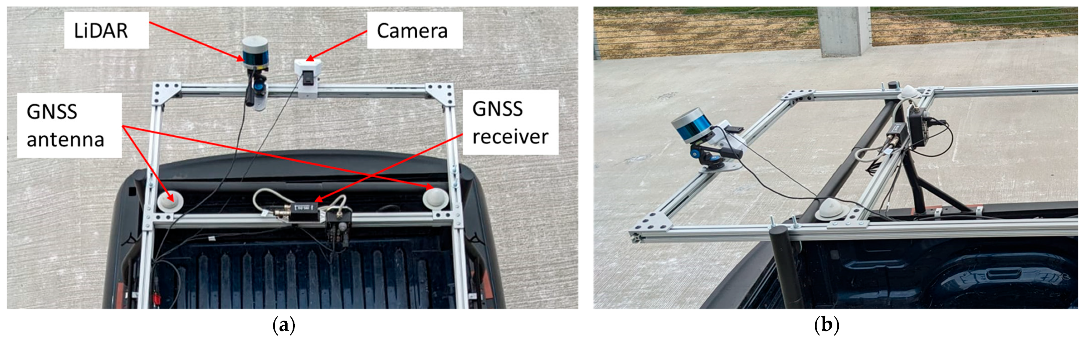
Funding

This research received no external funding.

Data Availability Statement

The original contributions presented in the study are included in the article, further inquiries can be directed to the corresponding author.

Conflicts of Interest

Author Sk Abu Talha conducted the research work presented in this paper when he was a student at the University of Cincinnati; he is currently employed by the company Applied Research Associates Inc. All authors declare that the research was conducted in the absence of any commercial or financial relationships that could be construed as a potential conflict of interest.

References

  1. American Automobile Association (AAA). Pothole Damage Fact Sheet; AAA: Heathrow, FL, USA, 2016. [Google Scholar]
  2. Bhatt, U.; Mani, S.; Xi, E.; Kolter, J.Z. Intelligent pothole detection and road condition assessment. arXiv 2017, arXiv:1710.02595. [Google Scholar]
  3. Dong, Q.; Huang, B.; Jia, X. Long-Term Cost-Effectiveness of Asphalt Pavement Pothole Patching Methods. Transp. Res. Rec. J. Transp. Res. Board 2014, 2431, 49–56. [Google Scholar] [CrossRef]
  4. Manasreh, D.; Nazzal, M.D.; Abu Talha, S.; Khanapuri, E.; Sharma, R.; Kim, D. Application of Autonomous Vehicles for Automated Roadside Safety Assessment. Transp. Res. Rec. J. Transp. Res. Board 2022, 2676, 255–266. [Google Scholar] [CrossRef]
  5. Koch, C.; Brilakis, I. Pothole detection in asphalt pavement images. Adv. Eng. Inform. 2011, 25, 507–515. [Google Scholar] [CrossRef]
  6. Buza, E.; Omanovic, S.; Huseinovic, A. Pothole detection with image processing and spectral clustering. In Proceedings of the 2nd International Conference on Information Technology and Computer Networks, Antalya, Turkey, 8–10 October 2013; Volume 810, p. 4853. [Google Scholar]
  7. Gomes Correia, M.; Ferreira, A. Road Asset Management and the Vehicles of the Future: An Overview, Opportunities, and Challenges. Int. J. Intell. Transp. Syst. Res. 2023, 21, 376–393. [Google Scholar] [CrossRef]
  8. Kim, T.; Ryu, S.K. Review and analysis of pothole detection methods. J. Emerg. Trends Comput. Inf. Sci. 2014, 5, 603–608. [Google Scholar]
  9. Kang, B.H.; Choi, S.I. Pothole detection system using 2D LiDAR and camera. In Proceedings of the 2017 Ninth International Conference on Ubiquitous and Future Networks (ICUFN), Milan, Italy, 4–7 July 2017; pp. 744–746. [Google Scholar]
  10. Li, Y.; Ibanez-Guzman, J. Lidar for Autonomous Driving: The Principles, Challenges, and Trends for Automotive Lidar and Perception Systems. IEEE Signal Process. Mag. 2020, 37, 50–61. [Google Scholar] [CrossRef]
  11. Zhang, Z.; Zheng, J.; Xu, H.; Wang, X. Vehicle Detection and Tracking in Complex Traffic Circumstances with Roadside LiDAR. Transp. Res. Rec. J. Transp. Res. Board 2019, 2673, 62–71. [Google Scholar] [CrossRef]
  12. Beltrán, J.; Guindel, C.; Moreno, F.M.; Cruzado, D.; Garcia, F.; De La Escalera, A. Birdnet: A 3d object detection framework from lidar information. In Proceedings of the 2018 21st International Conference on Intelligent Transportation Systems (ITSC), Maui, HI, USA, 4–7 November 2018; pp. 3517–3523. [Google Scholar]
  13. Royo, S.; Ballesta-Garcia, M. An Overview of Lidar Imaging Systems for Autonomous Vehicles. Appl. Sci. 2019, 9, 4093. [Google Scholar] [CrossRef]
  14. Yen, K.S.; Ravani, B.; Lasky, T.A. LiDAR for Data Efficiency; No. WA-RD 778.1; Washington State Department of Transportation, Office of Research and Library Services: Washington, DC, USA, 2011. [Google Scholar]
  15. He, Y.; Song, Z.; Liu, Z. Updating highway asset inventory using airborne LiDAR. Measurement 2017, 104, 132–141. [Google Scholar] [CrossRef]
  16. Díaz-Vilariño, L.; González-Jorge, H.; Bueno, M.; Arias, P.; Puente, I. Automatic classification of urban pavements using mobile LiDAR data and roughness descriptors. Constr. Build. Mater. 2016, 102, 208–215. [Google Scholar] [CrossRef]
  17. De Blasiis, M.R.; Di Benedetto, A.; Fiani, M.; Garozzo, M. Assessing of the road pavement roughness by means of LiDAR technology. Coatings 2020, 11, 17. [Google Scholar] [CrossRef]
  18. Alhasan, A.; White, D.J.; De Brabanter, K. Spatial pavement roughness from stationary laser scanning. Int. J. Pavement Eng. 2017, 18, 83–96. [Google Scholar] [CrossRef]
  19. Biçici, S.; Zeybek, M. An approach for the automated extraction of road surface distress from a UAV-derived point cloud. Autom. Constr. 2021, 122, 103475. [Google Scholar] [CrossRef]
  20. Ravi, R.; Bullock, D.; Habib, A. Pavement Distress and Debris Detection using a Mobile Mapping System with 2D Profiler LiDAR. Transp. Res. Rec. J. Transp. Res. Board 2021, 2675, 428–438. [Google Scholar] [CrossRef]
  21. Ravi, R.; Habib, A.; Bullock, D. Pothole mapping and patching quantity estimates using lidar-based mobile mapping systems. Transp. Res. Rec. 2020, 2674, 124–134. [Google Scholar] [CrossRef]
  22. Jocher, G. Yolov5. Available online: https://github.com/ultralytics/yolov5 (accessed on 10 March 2023).
  23. Wang, N.; Chen, T.; Liu, S.; Wang, R.; Karimi, H.R.; Lin, Y. Deep learning-based visual detection of marine organisms: A survey. Neurocomputing 2023, 532, 1–32. [Google Scholar] [CrossRef]
Figure 1. The data collection system: (a) top view, (b) side view.
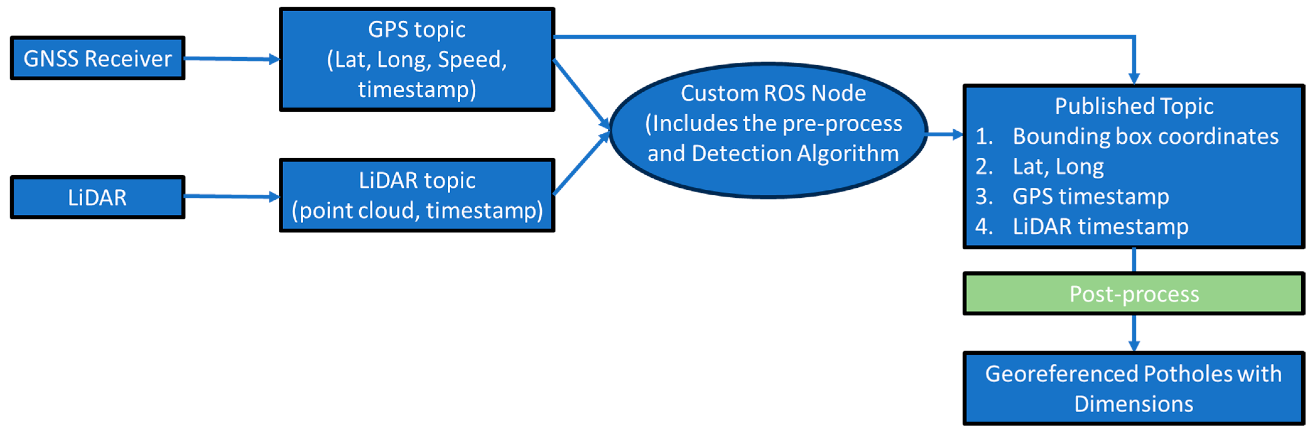
Buildings 14 01078 g001
Figure 2. Implementation of the proposed algorithm in ROS.
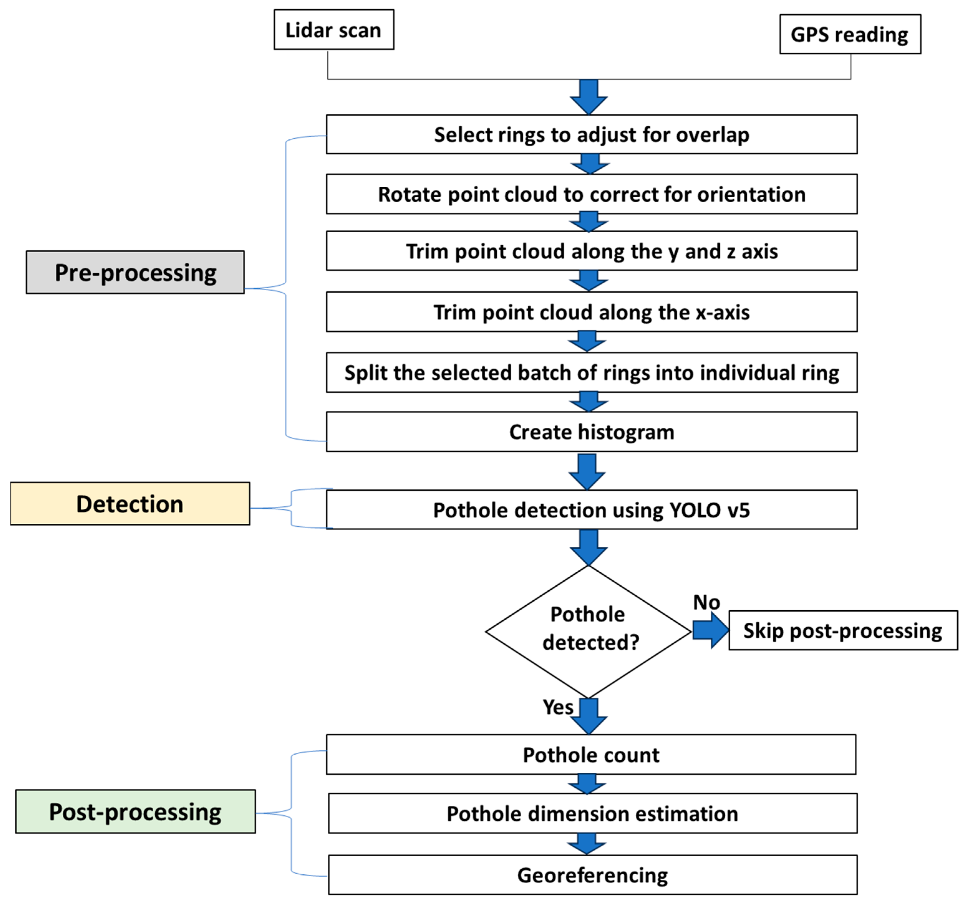
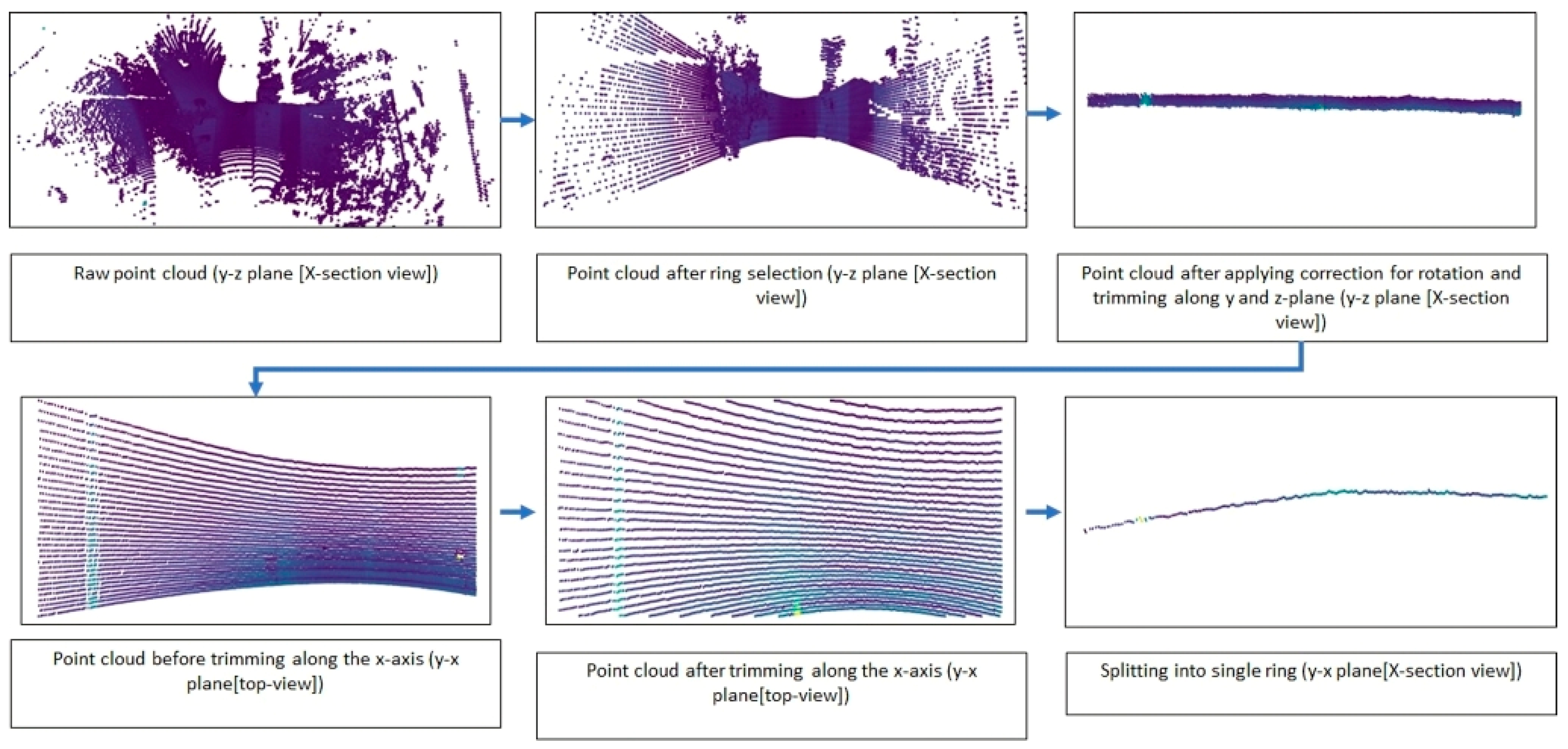
Buildings 14 01078 g002
Figure 3. Flowchart of the point cloud data processing.
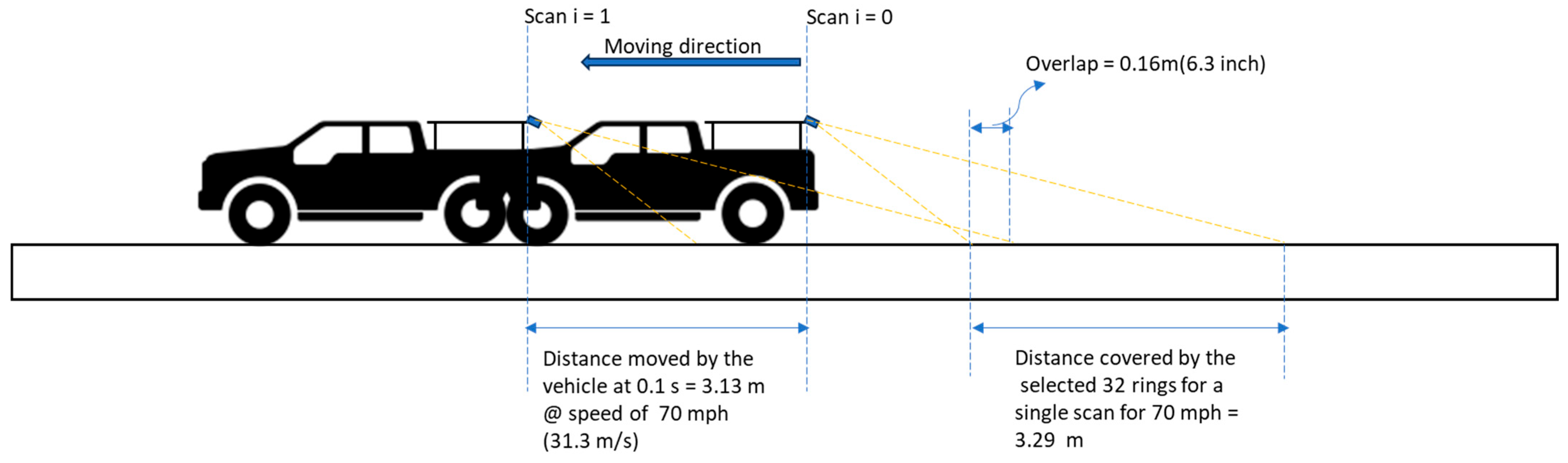
Buildings 14 01078 g003
Figure 4. Schematic diagram of the overlap between two subsequent LiDAR scans at a speed of 70 mph.
Buildings 14 01078 g004
Figure 5. Rotation and trimming of the point cloud.
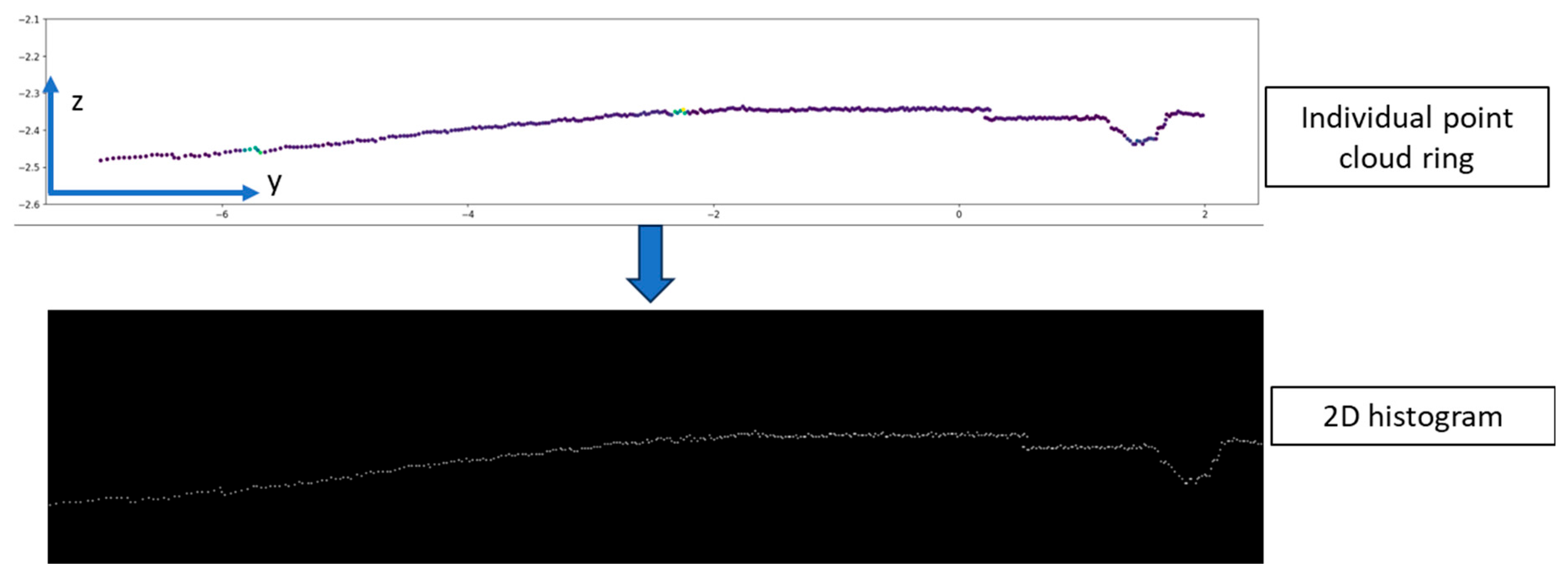
Buildings 14 01078 g005
Figure 6. Conversion of point cloud to 2D histogram.
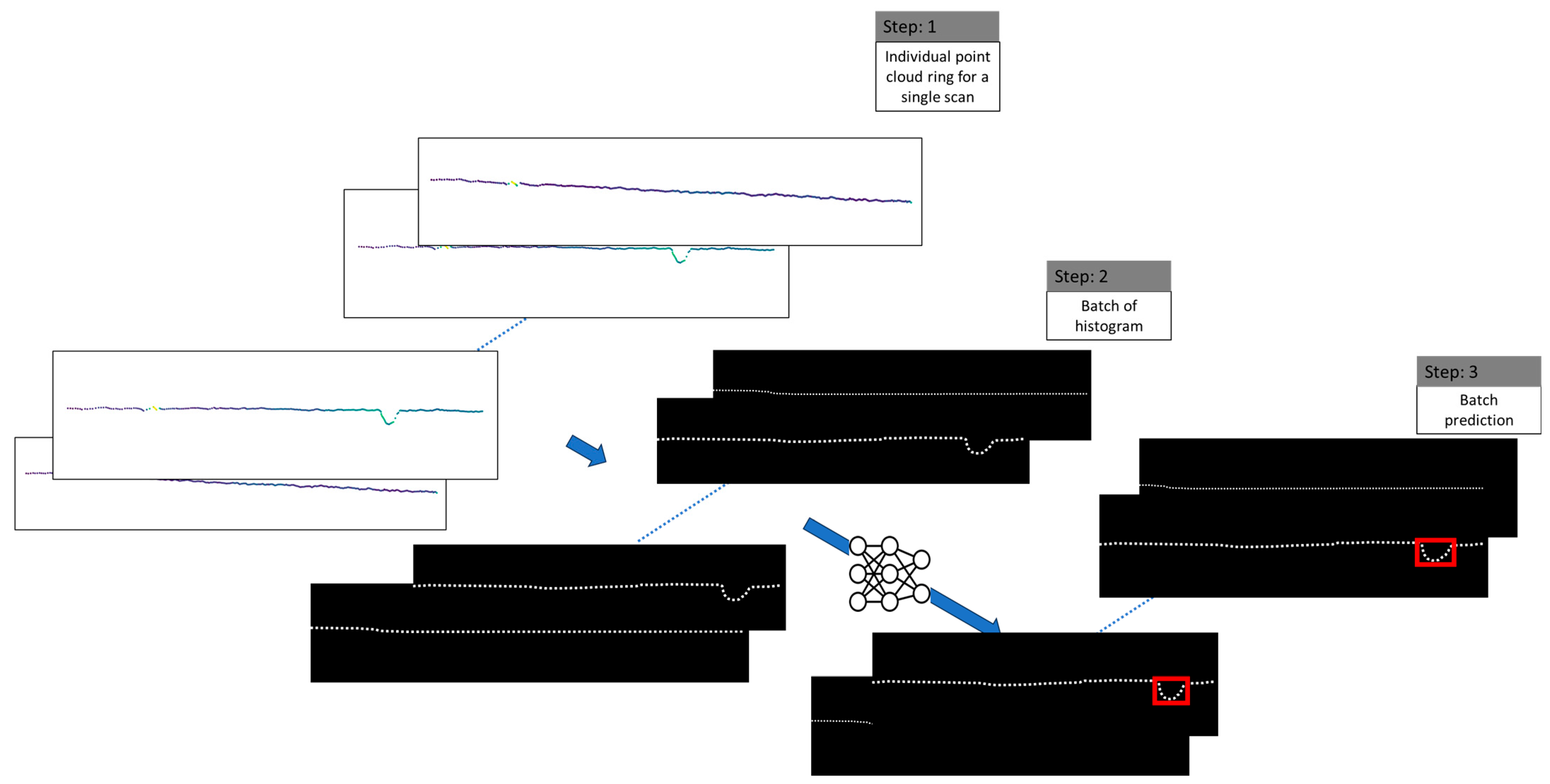
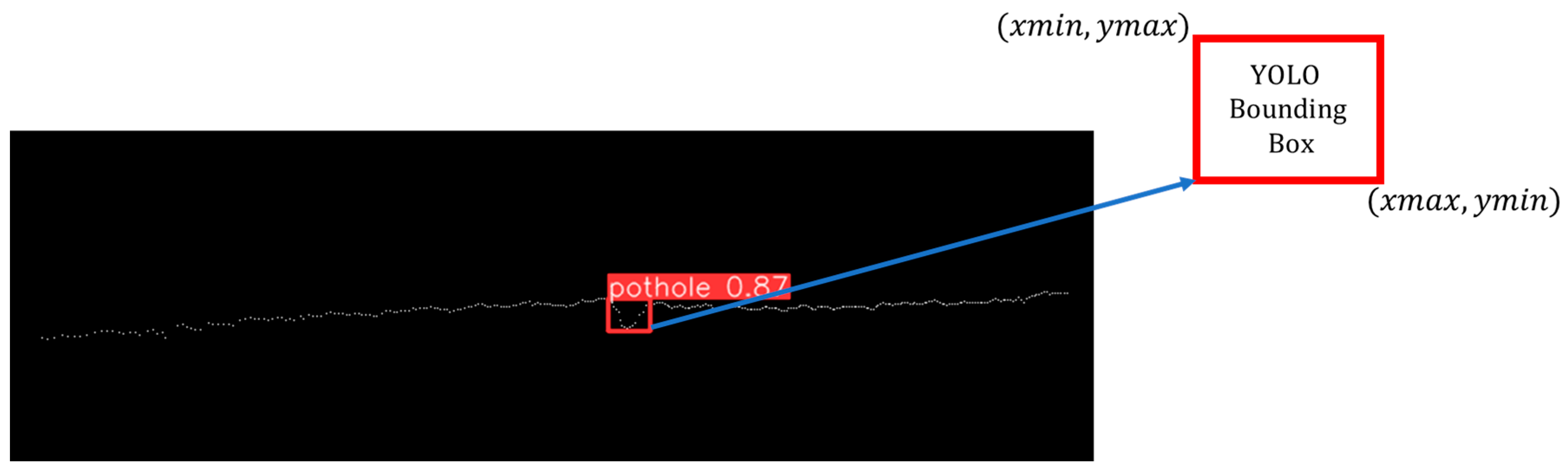
Buildings 14 01078 g006
Figure 7. Pothole detection from the 2D histograms.
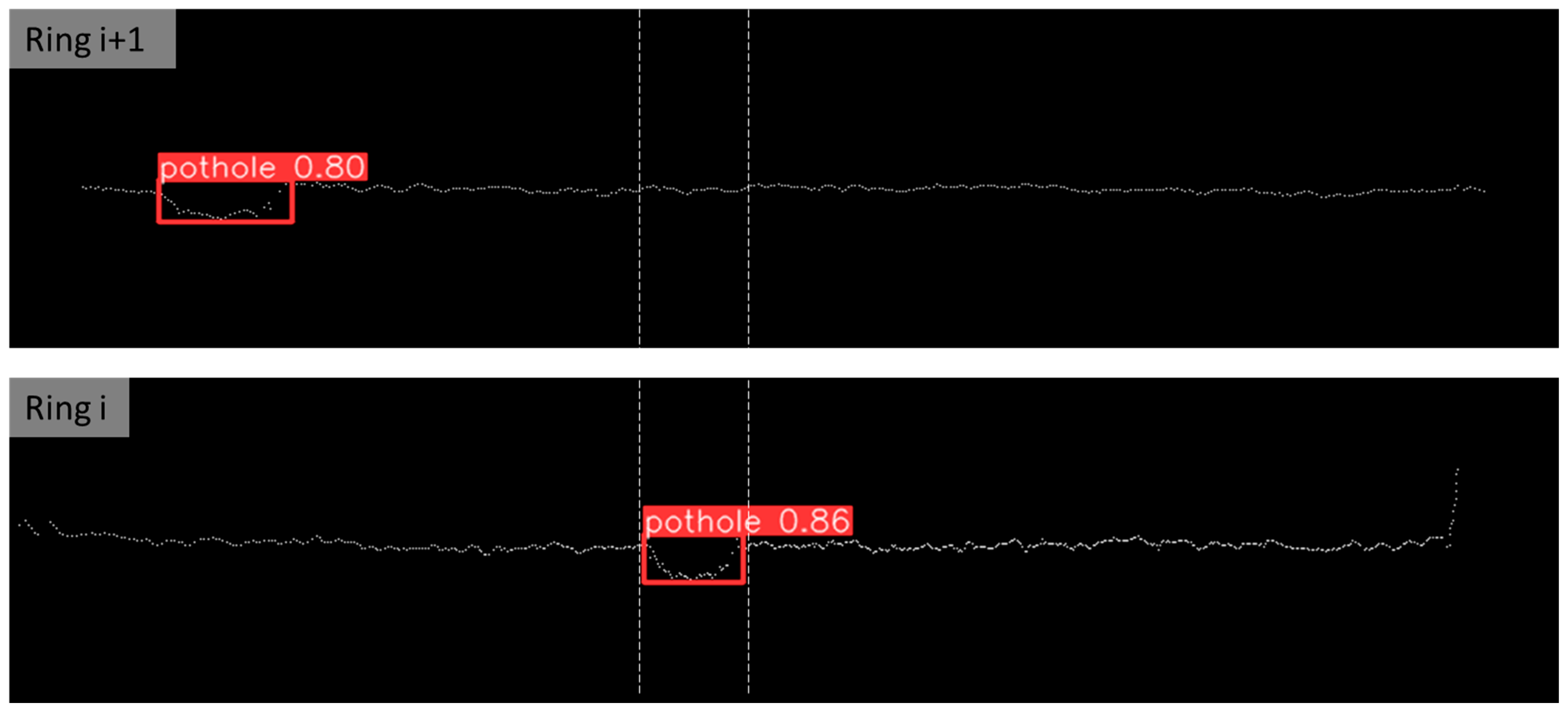
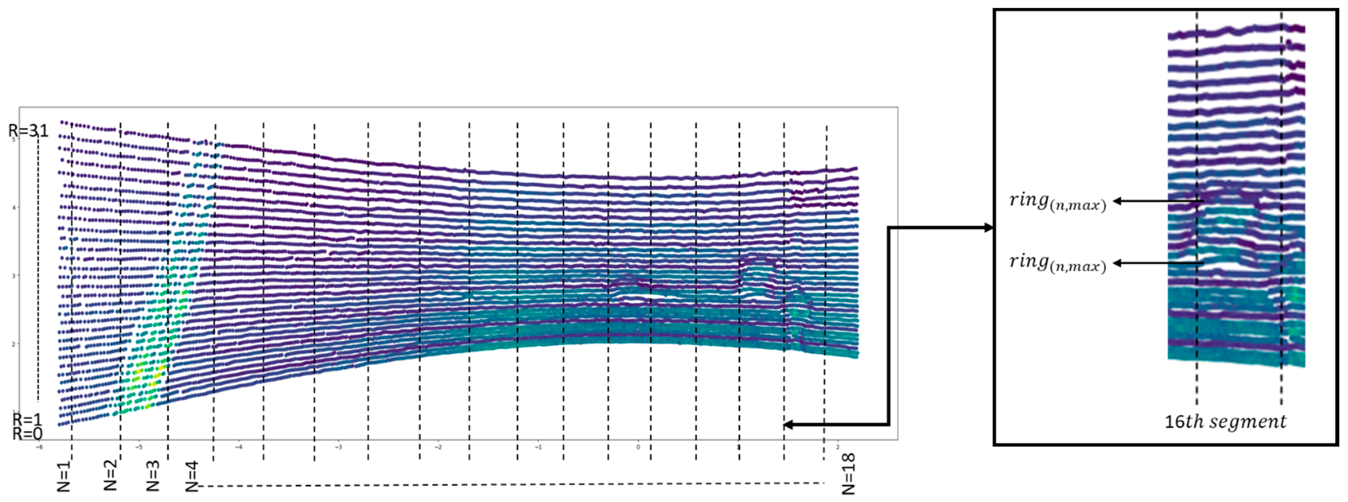
Buildings 14 01078 g007
Figure 8. Consecutive LiDAR rings corresponding to the same pothole (overlap).
Buildings 14 01078 g008
Figure 9. Subsequent LiDAR rings corresponding to different potholes (non-overlap).
Buildings 14 01078 g009
Figure 10. Implementation of the pothole counting algorithm.
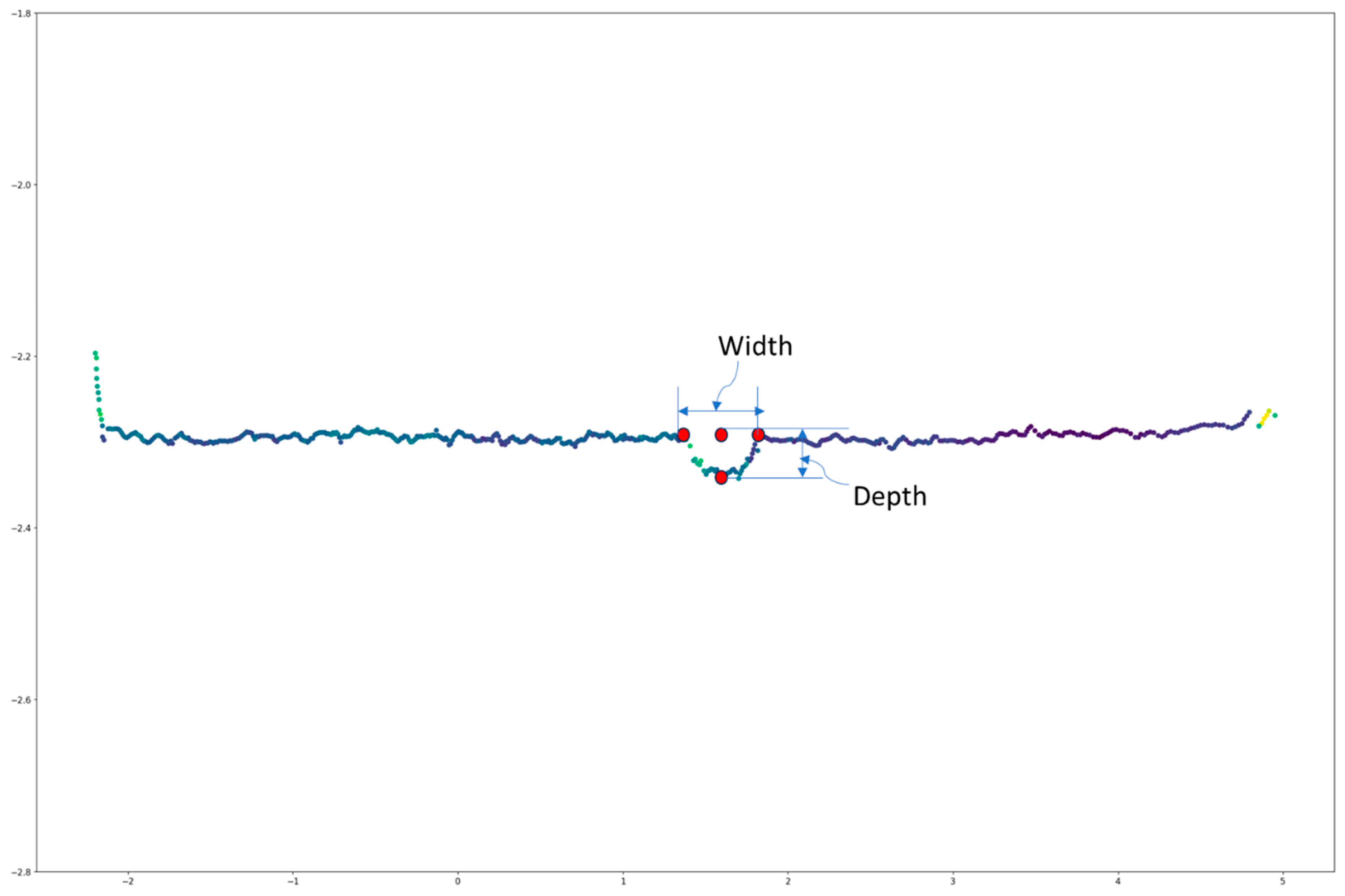
Buildings 14 01078 g010
Figure 12. Point-click procedure to obtain the actual dimension of the pothole.
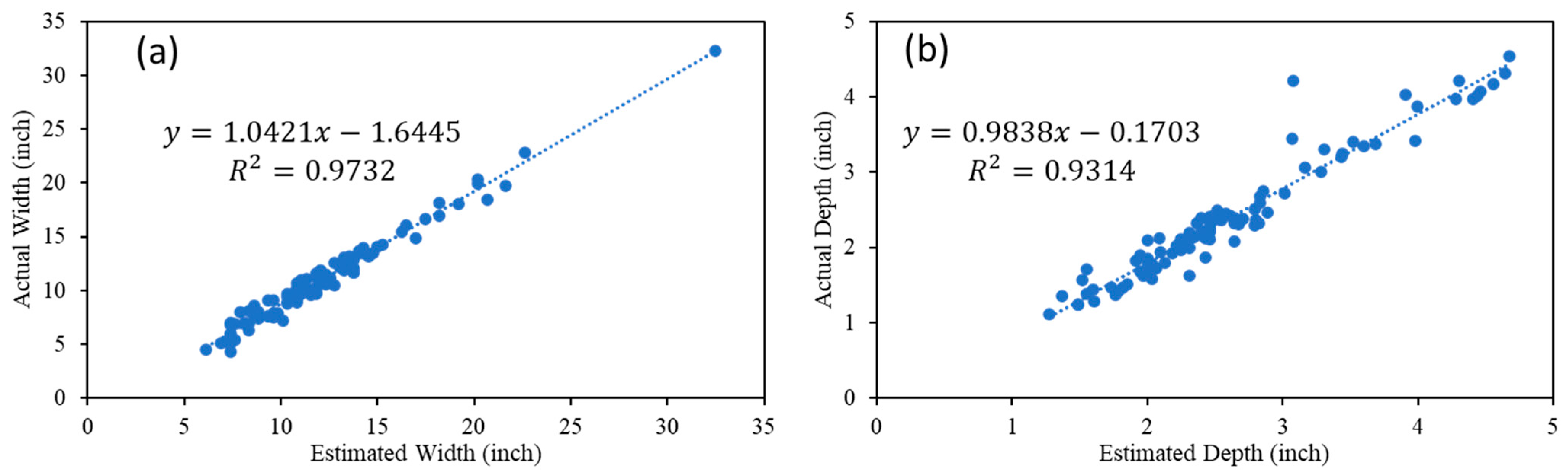
Buildings 14 01078 g012
Figure 13. (a) Correlation between actual and predicted width, and (b) correlation between actual and predicted depth.
Buildings 14 01078 g013
Figure 14. Determination of length.
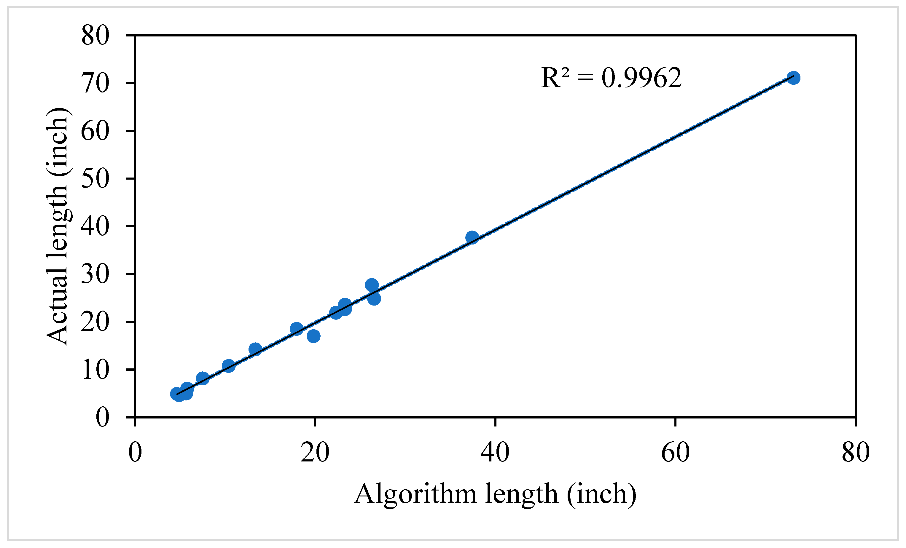
Buildings 14 01078 g014
Figure 15. Correlation between actual length and predicted length.
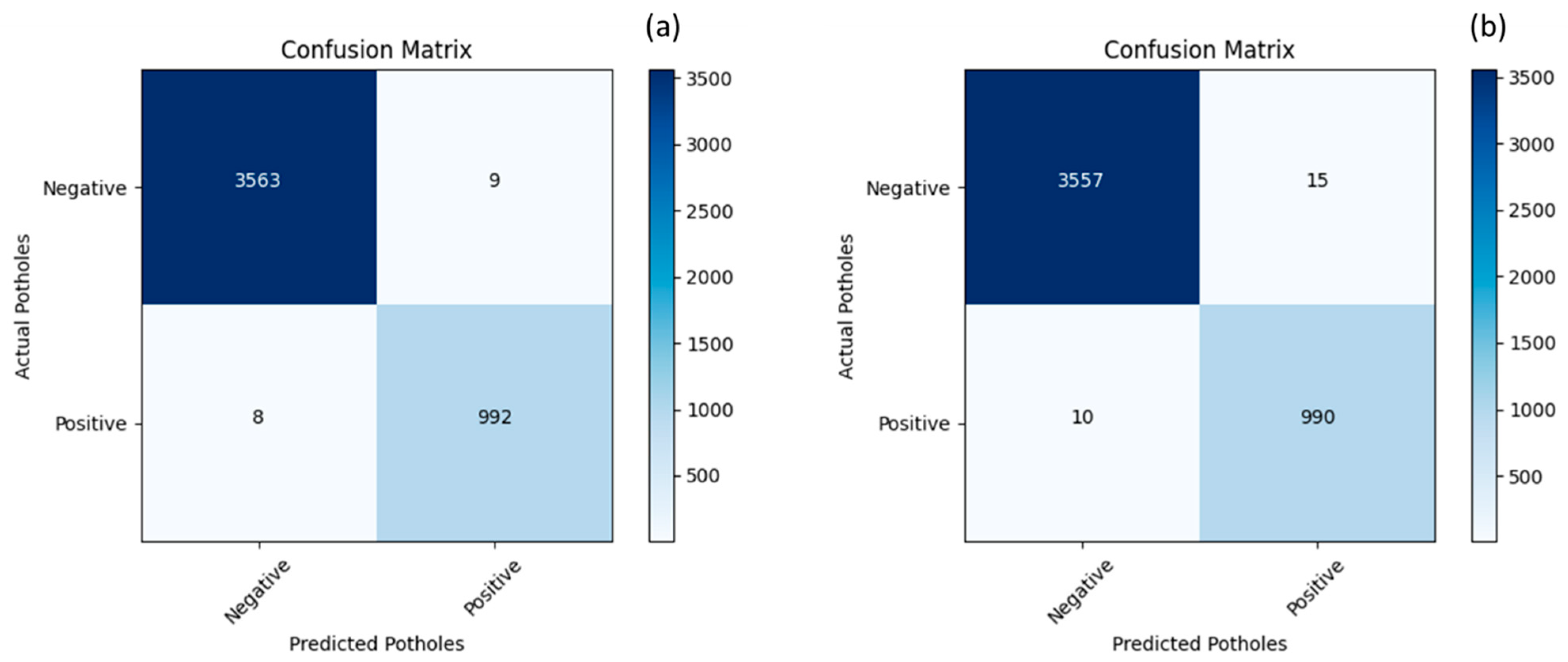
Buildings 14 01078 g015
Figure 16. Confusion matrix: (a) YOLO v5s, and (b) YOLO v5n.
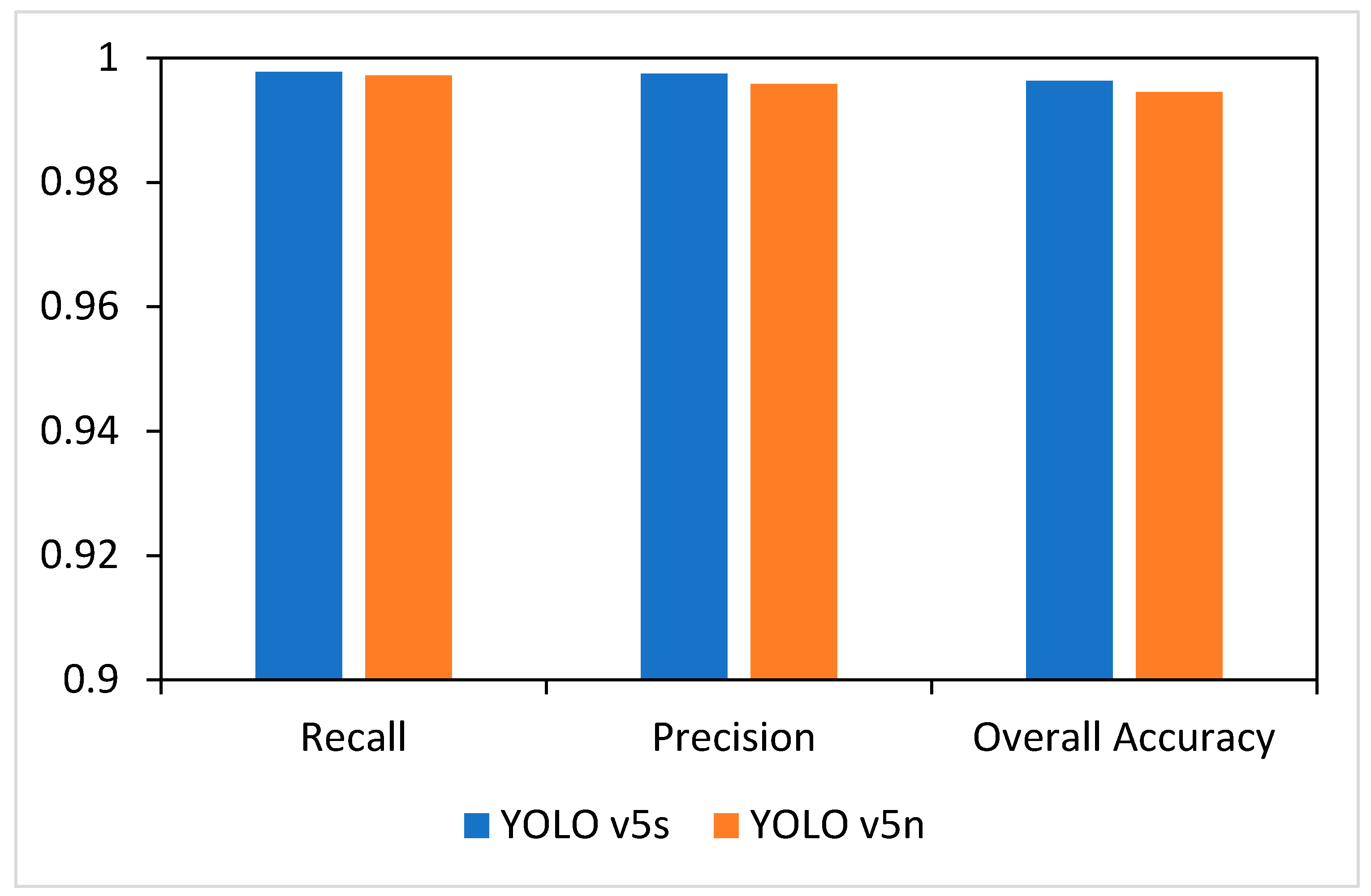
Buildings 14 01078 g016
Figure 17. Accuracy comparison between YOLO v5s and YOLO v5n.
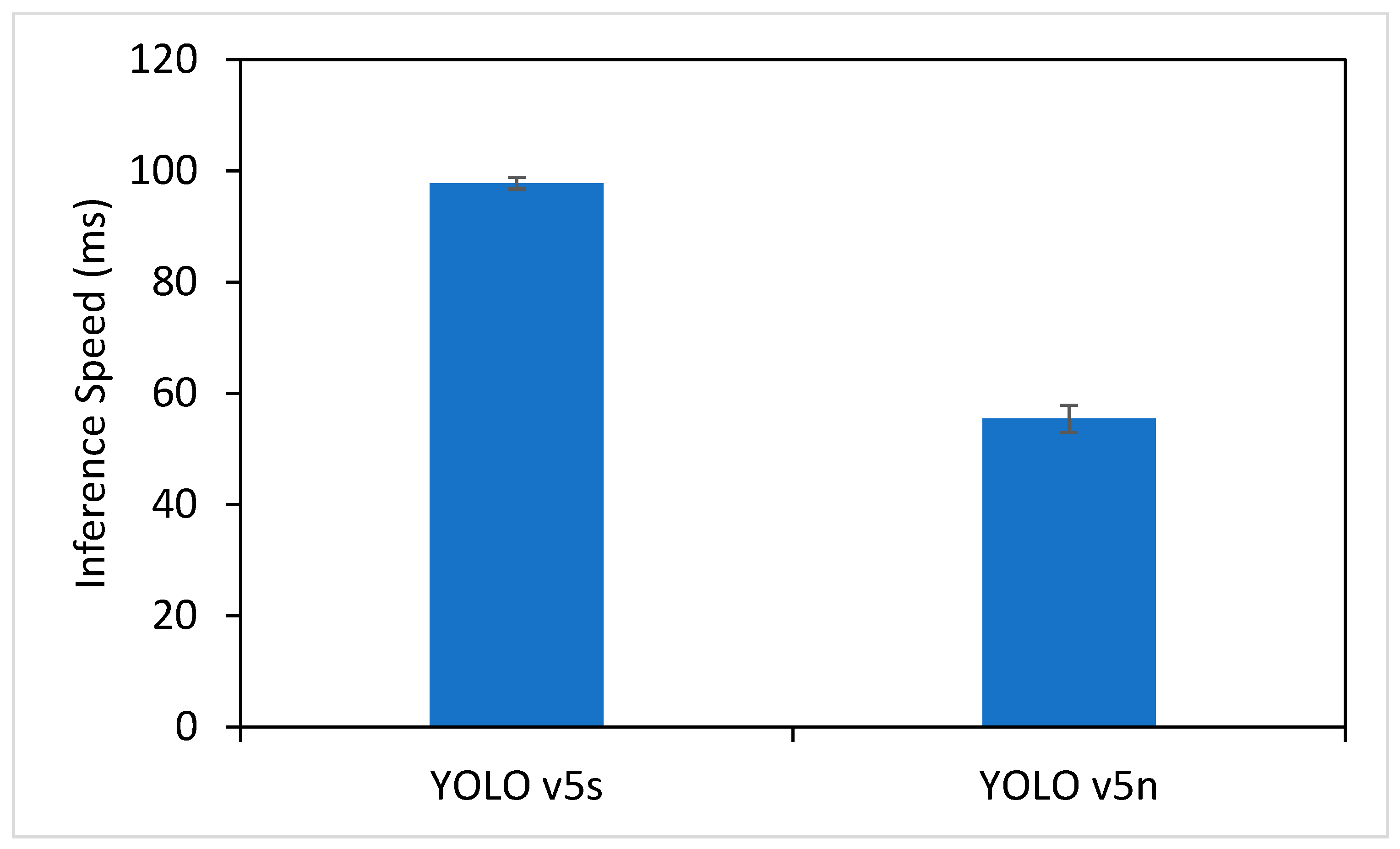
Buildings 14 01078 g017
Figure 18. Inference speed comparison between YOLO v5s and YOLO v5n.
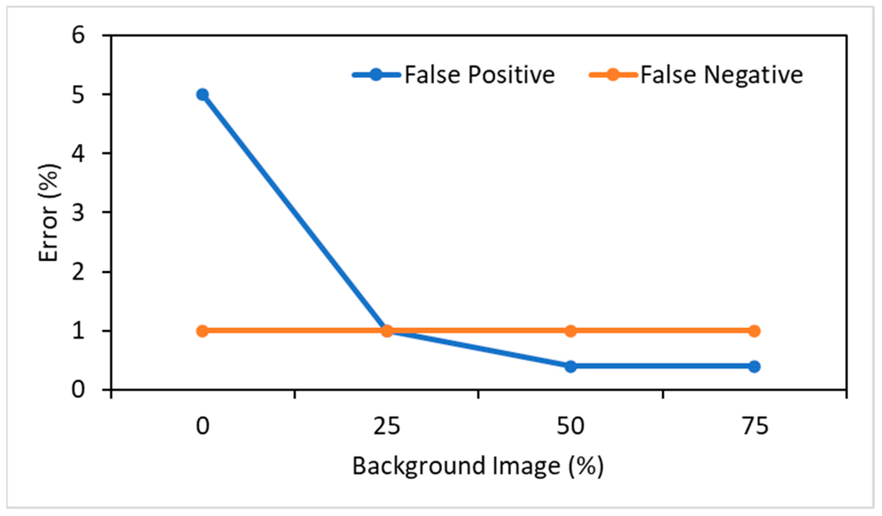
Buildings 14 01078 g018
Figure 19. Effect of background image percentage on false negative detection.
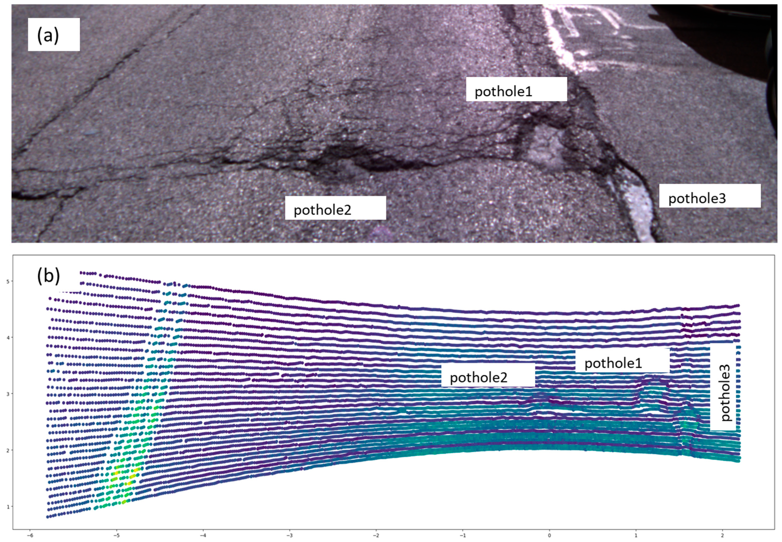
Buildings 14 01078 g019
Figure 20. Verification of the pothole count algorithm: (a) image of captured by camera (b) LiDAR scan corresponding to the image.
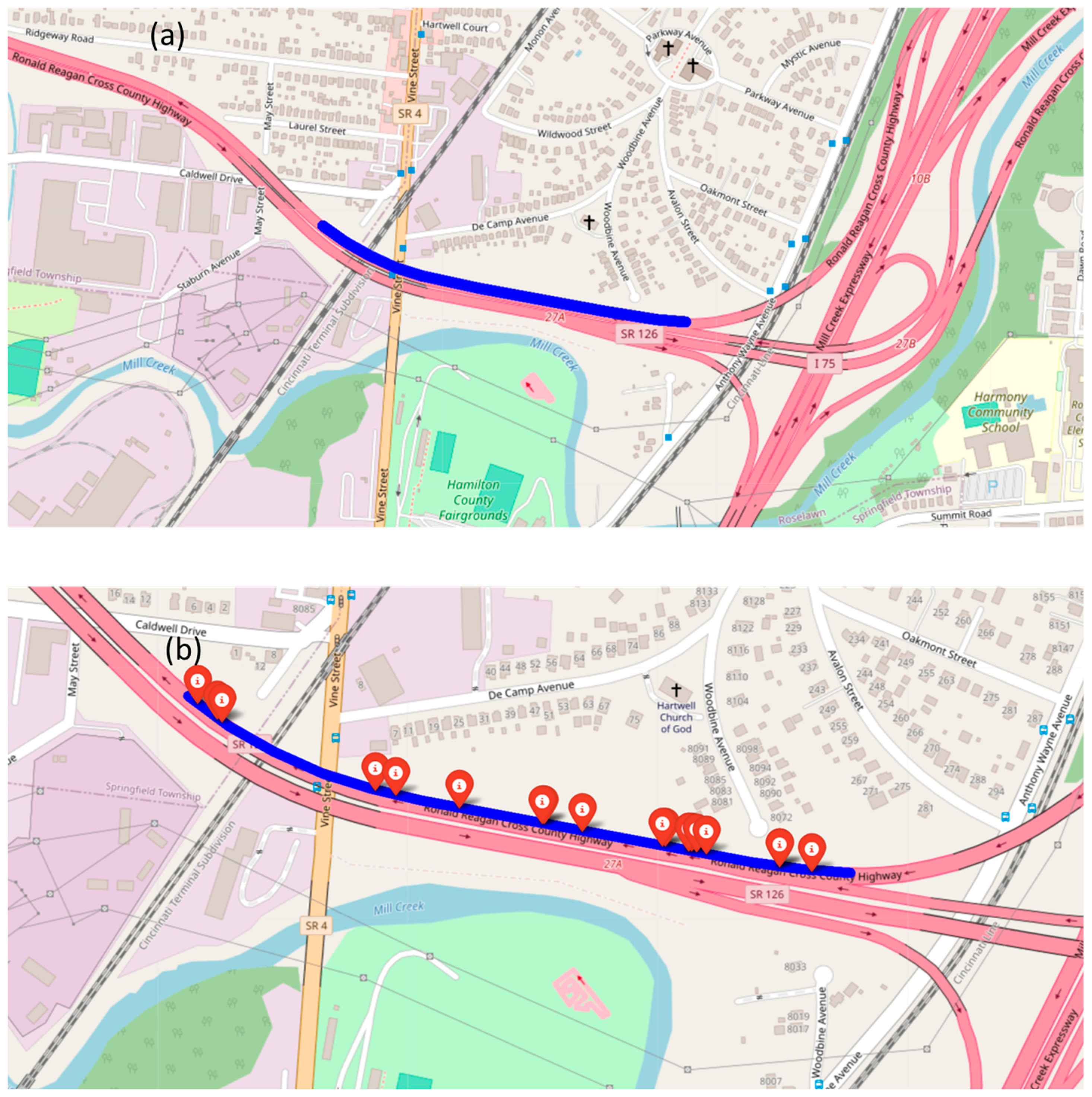
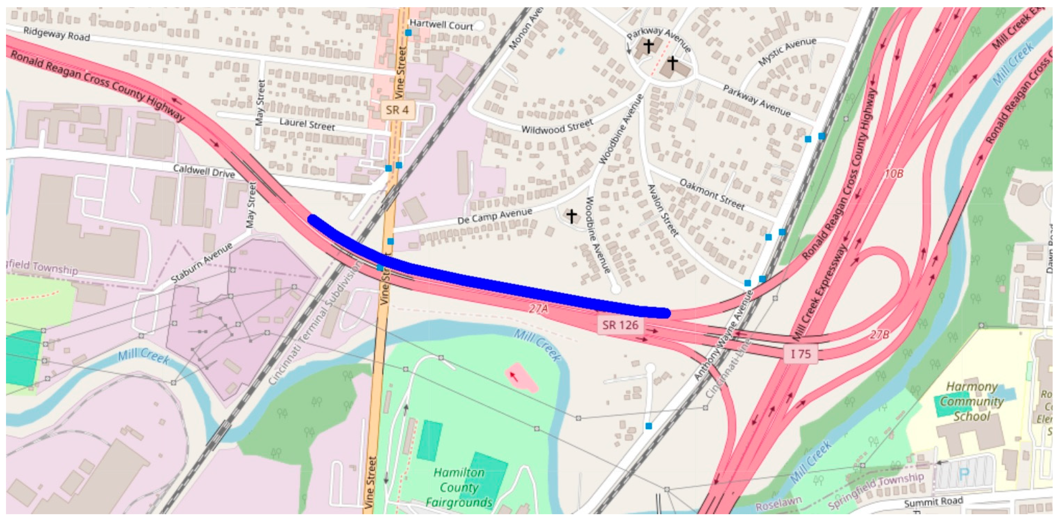
Buildings 14 01078 g020
Figure 21. (a) Location of the testing strip on State Route 126, and (b) detected potholes.
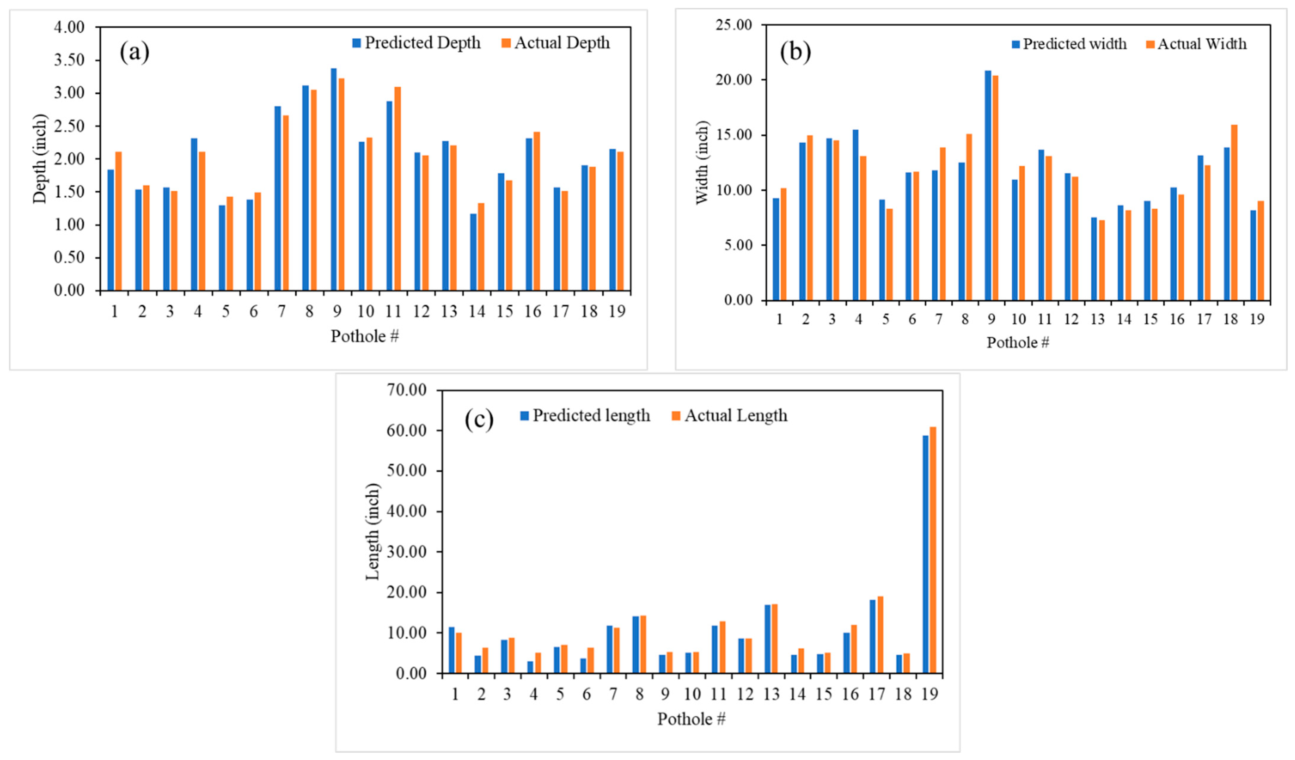
Buildings 14 01078 g021
Figure 22. Measured vs. predicted dimension: (a) depth, (b) width, and (c) length.
Buildings 14 01078 g022
Figure 23. Test strip (blue line) at Interstate 71 North.
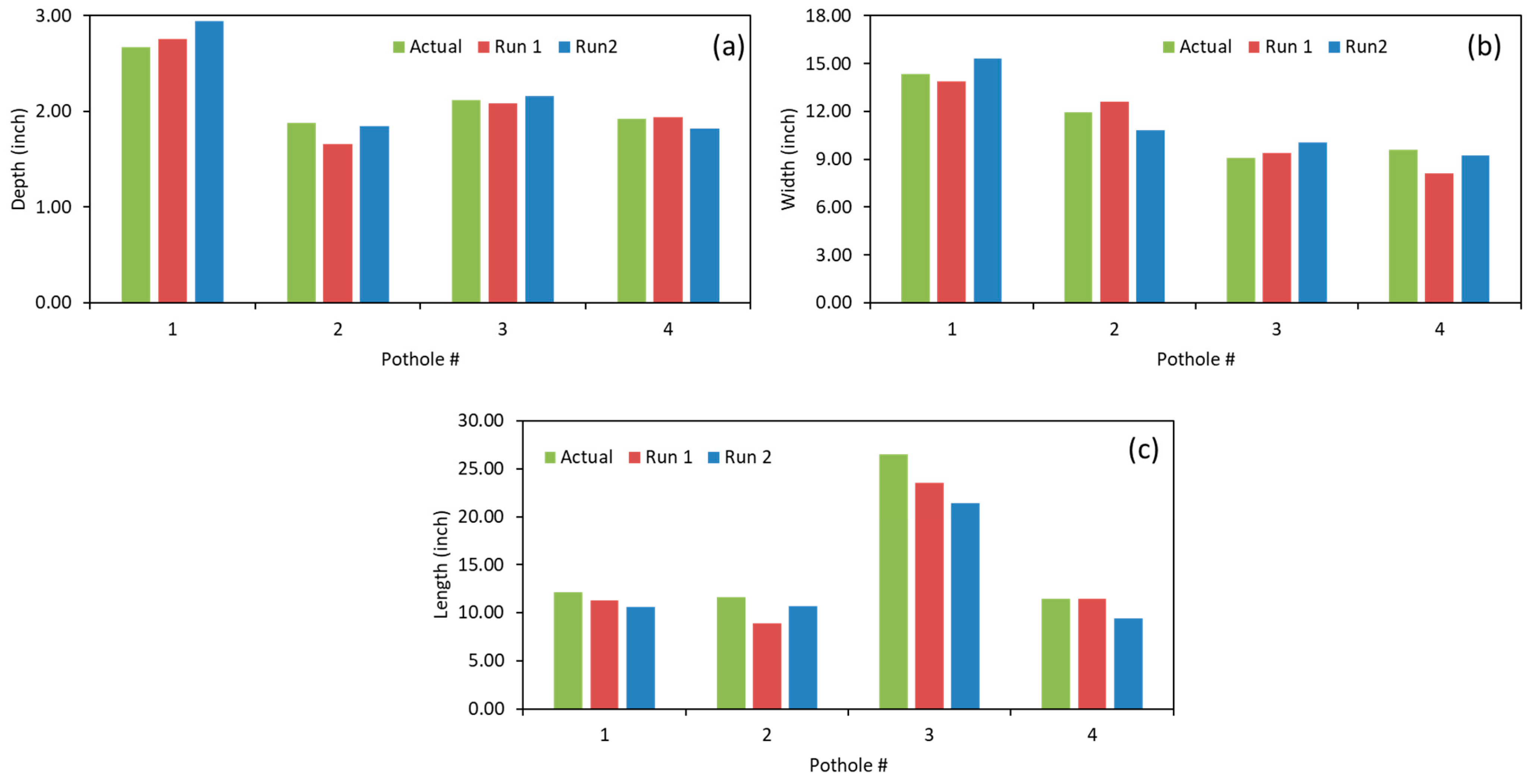
Buildings 14 01078 g023
Figure 24. Comparison between actual and predicted dimensions for Run 1 and Run 2 at 55 mph: (a) depth, (b) width, and (c) length.
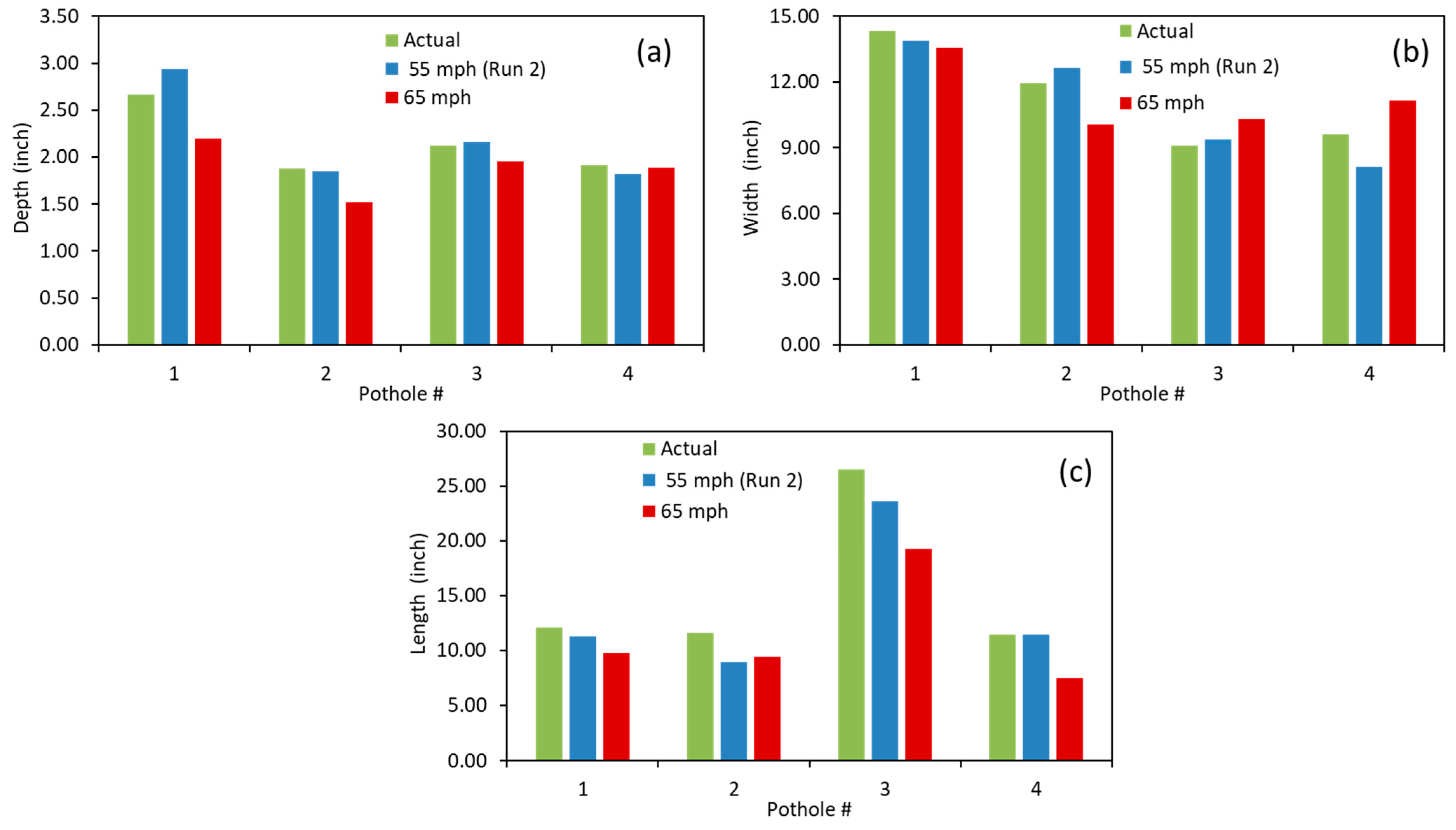
Buildings 14 01078 g024
Figure 25. Comparison between actual and predicted dimensions for Run 2 (55 mph) and run at 65 mph: (a) depth, (b) width, and (c) length.
Buildings 14 01078 g025
Table 1. Ring selection and area coverage at different speeds.
Speed (mph)Selected Ring #FOV along the Traffic DirectionOverlap
65 < speed ≤ 70#47–#783.190.17
60 < speed ≤ 65#48–#783.090.19
55 < speed ≤ 60#49–#782.870.19
≤55#53–#842.590.19
Table 2. Summary of the potholes detected from a single scan.
Pothole #Scan #Estimated Length (in)Actual Length (in)Difference in Length (in)Estimated Width (in)Actual Width (in)Difference in Width (in)Estimated Depth (in)Actual Depth (in)Difference in Depth (in)# of Rings
Pothole #115618.1618.600.4417.3116.221.092.112.060.057
Pothole #21567.588.100.5216.0815.100.981.821.790.034
Pothole #315632.6234.351.738.789.100.321.681.520.1613
Table 3. Summary of the potholes detected on Interstate 75 South.
Pothole IDPredicted Depth (Inches)Actual Depth (Inches)Error (Inches)Predicted Width (Inches)Actual Width (Inches)Error (Inches)Predicted Length (Inches)Actual Length (Inches)Error (Inches)No. of RingsLatitudeLongitude
12.082.110.039.3110.220.919.4410.100.66439.2050−84.4698
21.541.600.0614.3215.000.684.356.301.95339.2051−84.4706
31.571.510.0614.7314.500.238.378.930.56339.2052−84.4707
42.322.110.2115.5013.102.403.015.222.21239.2052−84.4708
51.301.430.139.188.330.856.517.100.59339.2052−84.4708
61.381.490.1111.5911.660.073.686.312.63239.2052−84.4708
72.802.660.1411.8213.892.0711.8111.360.45539.2052−84.4711
83.113.050.0612.5215.102.5814.1114.330.22739.2052−84.4711
93.373.220.1520.8620.410.454.605.330.73239.2053−84.4720
102.262.330.0710.9812.211.235.155.230.08339.2054−84.4724
112.883.100.2213.6813.100.5811.9312.931.00639.2054−84.4724
122.102.060.0411.5511.230.328.638.690.06339.2055−84.4733
132.272.210.067.527.320.2016.9917.220.23639.2056−84.4740
141.171.330.168.658.200.454.556.231.68339.2057−84.4742
151.791.680.119.068.330.734.835.100.27339.2063−84.4759
162.322.410.0910.279.620.6510.0312.102.07439.2063−84.4760
171.571.520.0513.1912.280.9118.2119.100.89539.2064−84.4762
181.901.880.0213.9015.952.054.554.930.38339.2050−84.4694
192.162.110.058.209.020.8258.9060.881.981839.2050−84.4698
Table 4. Summary of the potholes detected by two runs at 55 mph.
Pothole #Depth (Inches)Width (Inches)Length (Inches)
ActualRun 1Run 2Error (Run 1)Error (Run 2)ActualRun 1Run 2Error (Run 1)Error (Run 2)ActualRun 1Run 2Error (Run 1)Error (Run 2)
12.672.762.940.090.2714.3313.8915.340.441.0112.1011.3110.590.791.51
21.881.661.850.220.0311.9412.6310.850.691.0911.618.9310.662.680.95
32.122.082.160.040.049.119.3910.040.280.9326.5323.5821.382.955.15
41.921.941.820.020.109.618.129.221.490.3911.4711.469.410.012.06
Table 5. Locations of the potholes detected by the two runs at 55 mph.
Pothole #Run 1Run 2Difference in Pothole Location (m)
LatitudeLongitudeLatitudeLongitude
139.14084−84.483739.14085−84.48371.28
239.14092−84.483639.14094−84.48362.01
339.14144−84.483139.14145−84.48311.3
439.14328−84.472739.14328−84.47271.13
Table 6. Summary of the potholes detected at 55 mph and 65 mph.
Pothole #Depth (Inches)Width (Inches)Length (Inches)
Actual55 mph (Run 2)65 mph Error 55 mphError 65 mphActual55 mph (Run 2)65 mph Error 55 mphError 65 mphActual55 mph (Run 2)65 mph Error 55 mphError 65 mph
12.672.942.200.270.4714.3313.8913.580.440.7512.1011.319.790.792.31
21.881.851.520.030.3611.9412.6310.070.691.8711.618.939.432.682.18
32.122.161.950.040.179.119.3910.290.281.1826.5323.5819.302.957.23
41.921.821.890.100.039.618.1211.151.491.5411.4711.467.510.013.96
Table 7. Locations of the potholes detected by the two runs at 55 mph and 65 mph.
Pothole #55 mph (Run 2)65 mphDifference in Pothole Location (m)
LatitudeLongitudeLatitudeLongitude
139.1408514−84.483675739.1408598−84.48365262.2
239.1409417−84.483596639.1409237−84.4835962
339.1414454−84.483149639.1414564−84.48312382.53
439.1432827−84.472739739.1432729−84.47272031.99
Disclaimer/Publisher’s Note: The statements, opinions and data contained in all publications are solely those of the individual author(s) and contributor(s) and not of MDPI and/or the editor(s). MDPI and/or the editor(s) disclaim responsibility for any injury to people or property resulting from any ideas, methods, instructions or products referred to in the content.

