Predictive Modeling and Experimental Validation for Assessing the Mechanical Properties of Cementitious Composites Made with Silica Fume and Ground Granulated Blast Furnace Slag

Abstract

Using sustainable cement-based alternatives, such as secondary cementitious raw materials (SCMs), could be a viable option to decrease CO₂ emissions resulting from cement production. Previously conducted studies to determine the optimal mix designs of concrete primarily focused on either experimental approaches or empirical modeling techniques. However, in these experimental approaches, few tests could be performed for optimization due to time restrictions and lack of resources, and empirical modeling methods cannot be relied on without external validation. The machine learning-based approaches are further characterized by certain shortcomings, including a smaller number of data points, a less robust connection among the controlling factors, and a lack of comparative analyses among machine learning models. Furthermore, the literature on predicting the performance of concrete utilizing binary SCMs (silica fume (SF) and ground granulated blast furnace slag (GGBS)) is not available. Therefore, to address these drawbacks, this research aimed to integrate ML-based models with experimental validations for accurate predictions of the compressive strength (CS) and tensile strength (TS) of concrete that includes SF and GGBS as SCMs. Three soft computing techniques, namely the ANN, ANFIS, and GEP methods, were used for prediction purposes. Eight major input parameters, including the W/B ratio, cement, GGBS, SF, coarse aggregates, fine aggregates, superplasticizer, and the age of the specimens, were considered for modeling. The validity of the established models was assessed by using external experimental validation criteria, statistical metrics, and performance measures. In addition, sensitivity and parametric analyses were performed. Based on statistical measures, the ANFIS models outperformed other models with higher correlation and lower statistical error values. However, the GEP models exhibited superior performance compared to ANFIS and ANN with respect to the closeness of the RMSE, MAE, RSE, and R² values between the training, validation, and testing sets for both the CS and TS models. Experimental validation showed strong evidence for the applicability of the proposed models with an R² of 0.88 and error percentages of less than 10%. Sensitivity and parametric investigations demonstrated that the input variables exhibited the patterns described in the experimental dataset and the available literature. Hence, the proposed models are accurate, have better prediction performance, and can be used for design purposes.

1. Introduction

The construction sector is the primary source of global warming due to the significant CO₂ emissions produced during cement manufacturing [1,2]. Since the invention of modern-day cement in the early 1800s, its manufacture has consistently risen as a result of an increase in population, continuously growing urbanization, and extensive infrastructure construction. The global production of cement experienced a significant increase of 54%, rising from 1.6 billion tons in 2000 to 2.55 billion tons in 2006 [3,4]. In 2023, the worldwide manufacture of cement reached an incredible 4.1 billion tons, resulting in a total of 1.6 billion tons of CO₂ emissions, which is over three times higher than the 0.49 billion tons emitted in 1990, as reported by [5,6]. The International Energy Agency (IEA) predicts that global cement manufacturing will expand by an additional 12–23% by the year 2050 [7]. According to Hanifa et al. [8], China, India, Europe, and the United States were the leading countries in terms of CO₂ emissions from 2006 to 2021. Figure 1 shows the region-wise annual CO₂ emissions from cement industries in the last three decades. It can be seen that Asian countries had a significant growth in their CO₂ emissions, which was 5.3 times more than the initial emissions. In 2019, these countries accounted for 70.3% (1.73 Gt) of the overall CO₂ releases from the cement sector, as opposed to only 32% (0.28 Gt) in 1990. This rise is in line with their growing production of cement. It is known that the production of one ton of cement needs 1.5 tons of raw material, 140 kWh electricity, and 4000 MJ energy. Overall, the manufacture of cement accounts for around 8% of the world’s man-made CO₂ emissions and consumes around 3% of the world’s energy [9].

Cement has a negative long-term impact on the ecosystem due to CO₂ emissions and high energy consumption [11]. Therefore, minimizing CO₂ emissions from the cement manufacturing industry has become a primary concern for researchers [12]. Many approaches could be used to address this problem. One such viable strategy for minimizing the environmental impact associated with the cement industry is the utilization of SCMs as a partial substitute for cement in concrete [13,14,15]. The utilization of SCMs as a partial replacement for cement provides numerous benefits, such as higher strength, enhanced durability, financial advantages, and improved sustainability [16].

Industrial by-products, such as SF and GGBS, are proven to be the most effective SCMs as a substitute for cement in concrete. SF is produced in the smelting process of ferrosilicon or silicon alloy production, whereas GGBS is a by-product of blast furnaces. On average, annually, 1–1.25 million tons of SF and 230–260 million tons of GGBS are produced worldwide [17,18]. The inadequate management and disposal of these industrial residues can give rise to numerous environmental problems, including the emission of uncontrolled pollutants into the atmosphere during production and transportation, as well as soil and water pollution, if appropriate storage and disposal methods are not employed [19]. Furthermore, the excessive accumulation of significant volumes of SF and GGBS waste can exert pressure on waste management systems, resulting in earlier saturation of landfills. This, in turn, can have adverse effects on communities. Therefore, the implementation of efficient methods for handling these wastes and the exploration of sustainable applications, such as incorporating them as SCMs in concrete, can be beneficial by reducing the environmental concerns associated with SF, GGBS, and the cement industry. For instance, Akhtar et al. [20] investigated that substituting 10% of SF in 2.2 billion tons of concrete decreased CO₂ emissions by 39 million tons. In another study [21], it has been stated that replacing 50% of GGBS in concrete with OPC can reduce around 0.5 tons of the CO₂ emissions per ton of concrete. Considering the environmental drawbacks of the cement industry and the benefits of employing SCMs in concrete, it is imperative to develop robust and reliable methods for sustainable construction practices.

Recent advances in machine learning (ML) techniques have led to the development of precise and reliable models for predicting the properties of various cement-based composites containing SCMs [22]. For instance, several ML techniques, including GEP [23], support vector machines (SVMs) [24], multilayer perception neural networks (MLPNNs) [25], deep learning (DL) [26], the ANFIS, ANNs, and multi-expression programming (MEP) [27], have been effectively employed to estimate the mechanical characteristics of concrete incorporated with SCMs. Recently, ANN and ANFIS ML approaches have been used successfully to identify and generalize complex patterns in data. Hence, they can be efficiently utilized to estimate the properties of concrete. Shahmansouri et al. [28] employed ANN models to predict the CS of geopolymer concrete (GPC) using an experimental database of 117 specimens from 39 different mixtures containing varying proportions of GGBS, SF, and natural zeolite. They compared the ANN-estimated CS with the actual results and observed that the ANN model accurately predicted the CS of GPC. Amlashi et al. [29] used three soft computing models: an M5 model tree (M5MT), an ANN, and multivariate regression, to estimate the elastic modulus, CS, and slump of plastic concrete. Their findings indicate that the ANN model had superior accuracy in predicting all three parameters compared to the other models. Mahesh et al. [30] used ANN models to estimate the elastic modulus and CS of fiber-reinforced concrete. The models were developed using 158 and 140 experimental results for the elastic modulus and CS, respectively. The outcomes of their study show the superior predictive capabilities of the ANN, as it exhibits minimal variation from the actual values, with R² values of 0.96 and 0.97 for the elastic modulus and CS, respectively. Topçu et al. [31] explored ANN and fuzzy logic algorithms in order to accurately predict the CS and TS of recycled aggregate concrete incorporated with SF. The models were constructed using experimental data from 210 specimens with 35 different mix designs. For the purpose of prediction, the study utilized eight input parameters and examined the strength properties at various time intervals (3, 7, 14, 28, 56, and 90 days). The outcomes of the models indicate that ANN and fuzzy logic algorithms possess considerable potential in accurately forecasting the strength properties of concrete. Dao et al. [32] focused on predicting the CS of GPC through the utilization of two ML techniques: the ANN and ANFIS techniques. For the model development, 210 samples were used. The outputs of the ANN and ANFIS were evaluated based on several statistical measures, such as R² and MAE values. The findings indicate that both models exhibited substantial potential in anticipating the CS of GPC. However, the ANFIS outperformed the ANN model with a marginally lower MAE of 1.655 MPa compared to 1.989 MPa and a higher R² of 0.879 compared to 0.851. Overall, the study provides evidence to support the efficacy of the ANFIS and ANN models as predictive tools for estimating the CS of GPC. Using ANNs, Sadowski et al. [33] projected the CS of concrete comprising waste quartz dust. The ANN models revealed strong correlation values (R) of 0.93, 0.91, and 0.94 for the training, testing (evaluation), and validation stages, respectively, indicating that the CS of green concrete utilizing waste mineral dust can be evaluated accurately using these models. Despite the reliable correlation proposed by these models, no empirical formula was suggested for their practical use. This is because of the sophisticated architecture of ANNs and the ANFIS, which is also regarded as a significant barrier to the widespread adoption of ANN and ANFIS models [34]. Multi-collinearity is also another drawback of these modeling techniques. Furthermore, ANNs and ANFIS are categorized as “black-box models” due to their incapability to demonstrate fundamental physical mechanisms, limited transparency, and inability to generate closed-form prediction equations [35].

Evolutionary modeling approaches such as GEP, influenced by Darwin’s idea of natural selection, have gained the attention of researchers in recent years. Unlike “black-box” models such as ANNs and the ANFIS, GEP gives predictive equations that provide valuable information about the connections between input parameters and the desired output [36]. GEP-extracted mathematical formulas can be used in practice with improved prediction efficiency. Nafees et al. [23] used MLPNN, GEP, and ANFIS models to forecast the CS and TS of concrete incorporated with silica fume by utilizing a database comprising 283 and 145 data points for CS and TS, respectively. It was reported that all three models showed a notable level of accuracy in their predictive capabilities. Nevertheless, the GEP models demonstrated their superiority by yielding significantly higher R² values than the other methods. According to the authors, the GEP method developed predictive equations for each outcome, which can be used to pre-design SF concrete mixtures in the future. Awoyera et al. [37] employed two ML models, GEP and an ANN, to predict the flexural strength, CS, and TS of self-compacted geopolymer concrete. The prediction outcomes were compared using statistical values of the mean square error (MSE) and R². The author concluded that GEP models are more reliable as they gave fewer errors and provided empirical relationships for forecasting the properties of concrete. Shahmansouri et al. [38] developed numerical models using GEP to predict the CS of geopolymer concrete containing GGBS. A total of 351 data records, with the five most important input parameters, were employed to create the models. The efficacy and generalization ability of the models was assessed based on sensitivity and parametric analyses. The study’s findings indicate that GEP models can be used as an effective tool for promoting sustainability in the construction sector as they provide robust and strong empirical correlations.

Based on the aforementioned literature analysis, it is evident that numerous researchers have employed ML methodologies to forecast the mechanical characteristics of concrete that incorporate supplementary cementitious materials (SCMs) by employing traditional machine learning techniques. The aforementioned investigations were characterized by certain shortcomings, including a smaller number of data points, a less robust connection among the controlling factors, the non-availability of GEP-based predictive equations, and a lack of comparative analyses and experimental validation. Furthermore, as per the authors’ knowledge, studies in the literature about predicting the performance of concrete utilizing binary SCMs (silica fume and GGBS) are not available. Therefore, for the first time, this study employed three distinct computational methodologies, including ANN, ANFIS, and GEP techniques, to develop models that can accurately and precisely forecast the CS and TS of concrete incorporated with SF and GGBS. Each model’s predictive performance was assessed using various statistical performance measures and experimental testing for cross-validation in the laboratory. Moreover, sensitivity and parametric analyses were conducted to determine the influence of input variables on the CS and TS of concrete incorporated with SF and GGBS. The availability of reliable and precise ML techniques to anticipate the properties of concrete containing SF and GGBS will promote sustainability and save money and time.

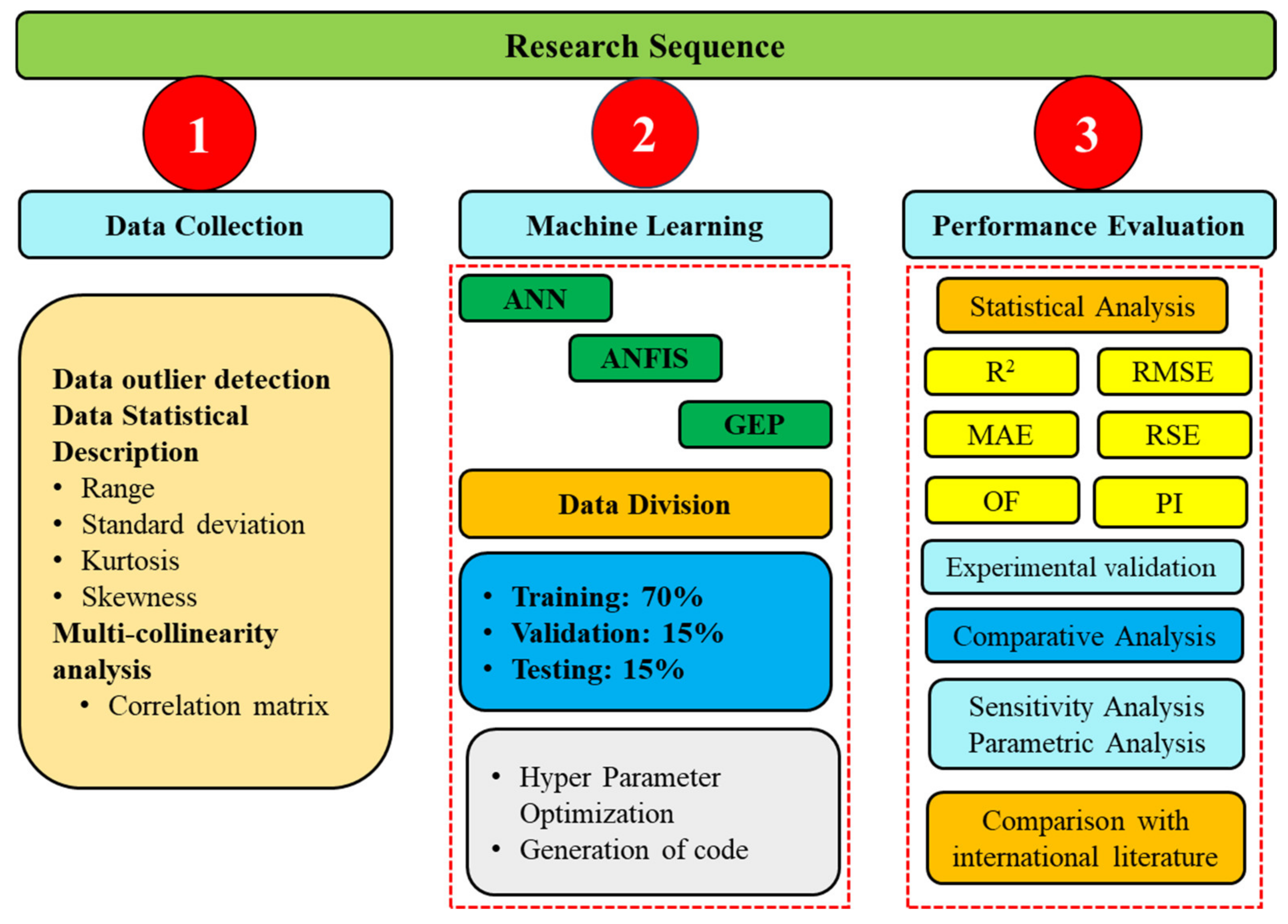
2. Research Methodology

The process used to develop the modeling techniques for forecasting the CS and TS of concrete containing SF and GGBS is described in this section. Initially, a detailed description of the data collection is provided, followed by a general review of the ML techniques (ANN, ANFIS, and GEP) employed in this study. Thereafter, performance measurement and experimental validation criteria for the models are discussed. Figure 2 shows a detailed overview of the methodological procedure followed in this research.

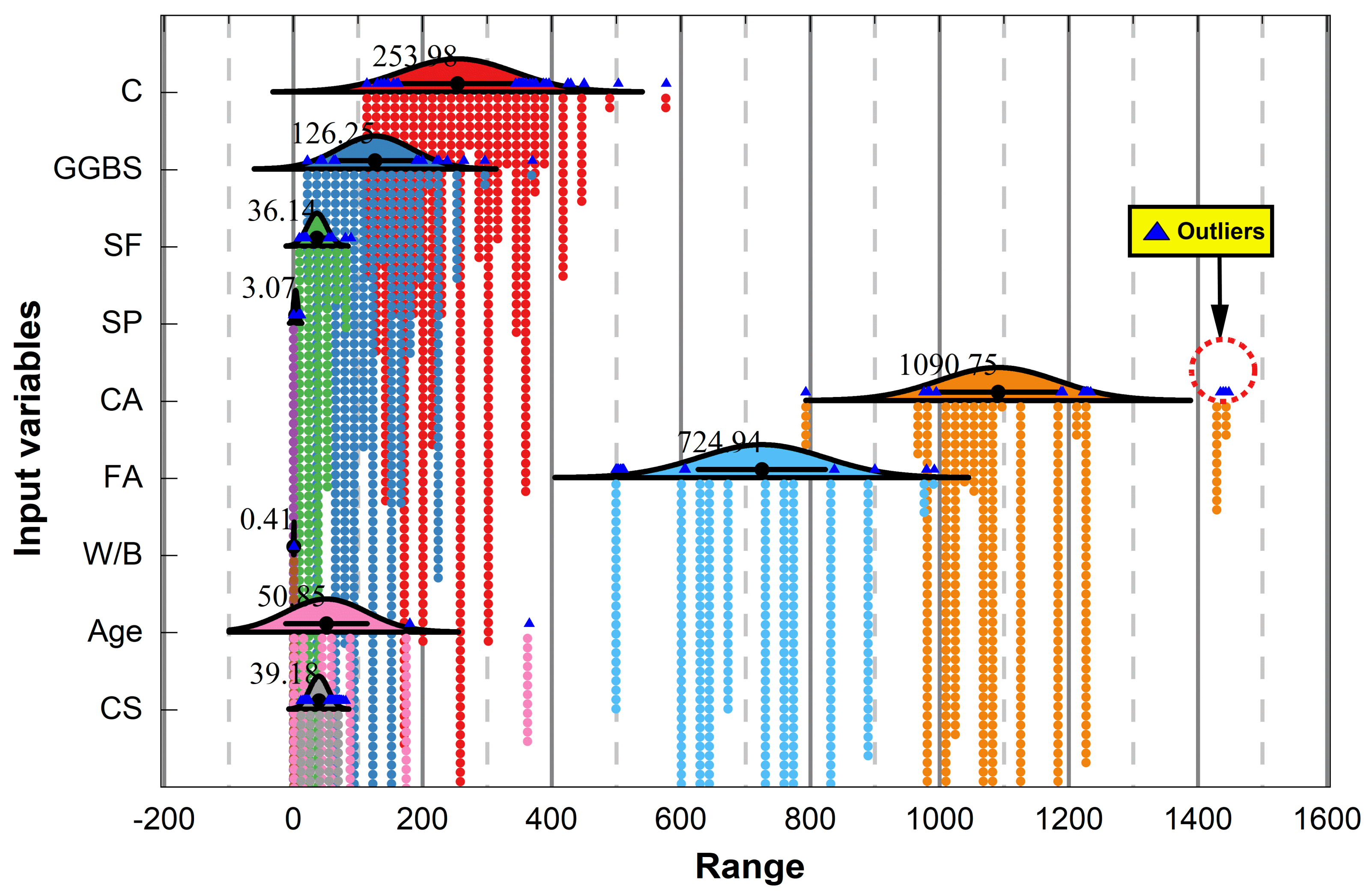
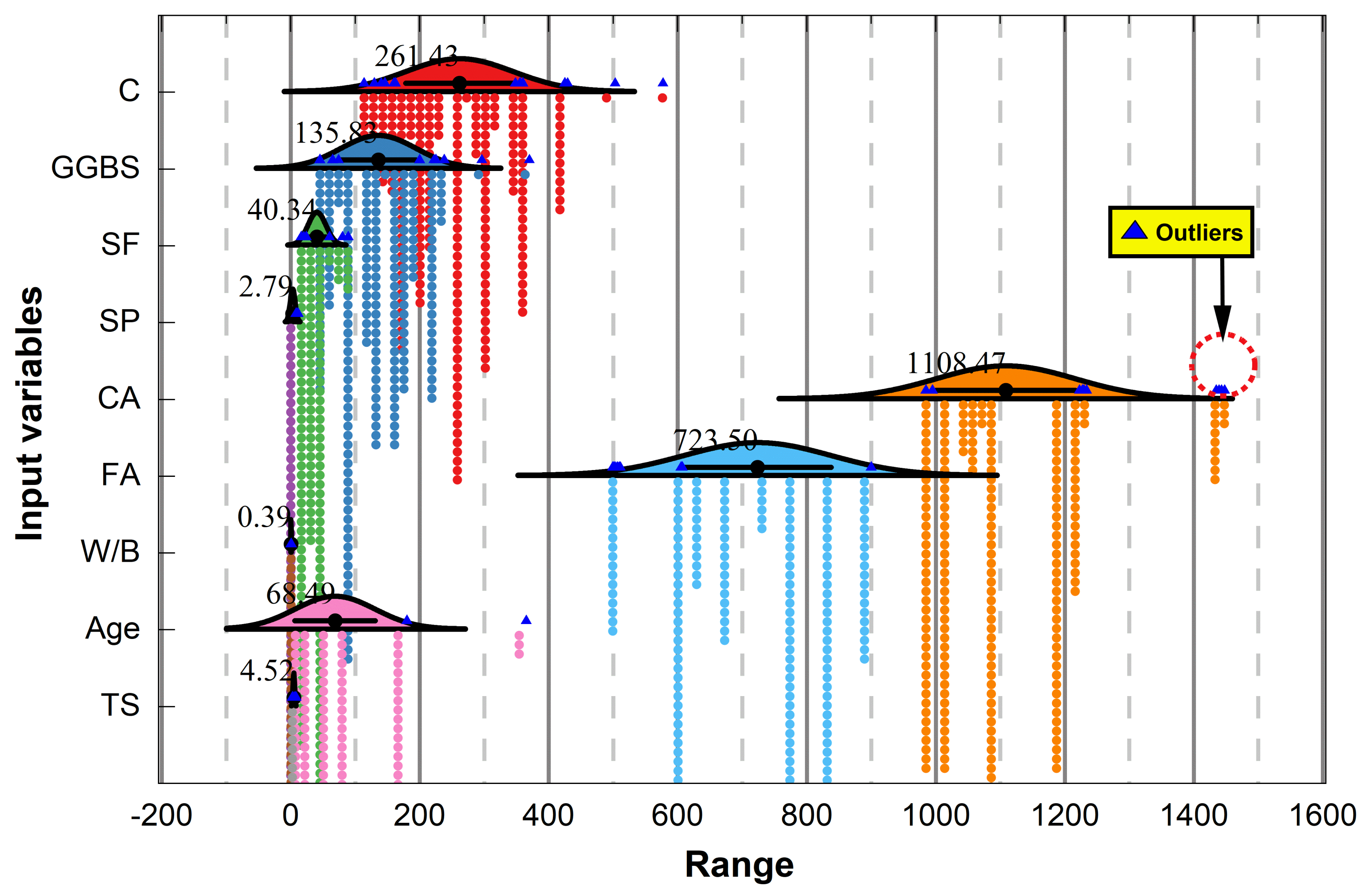
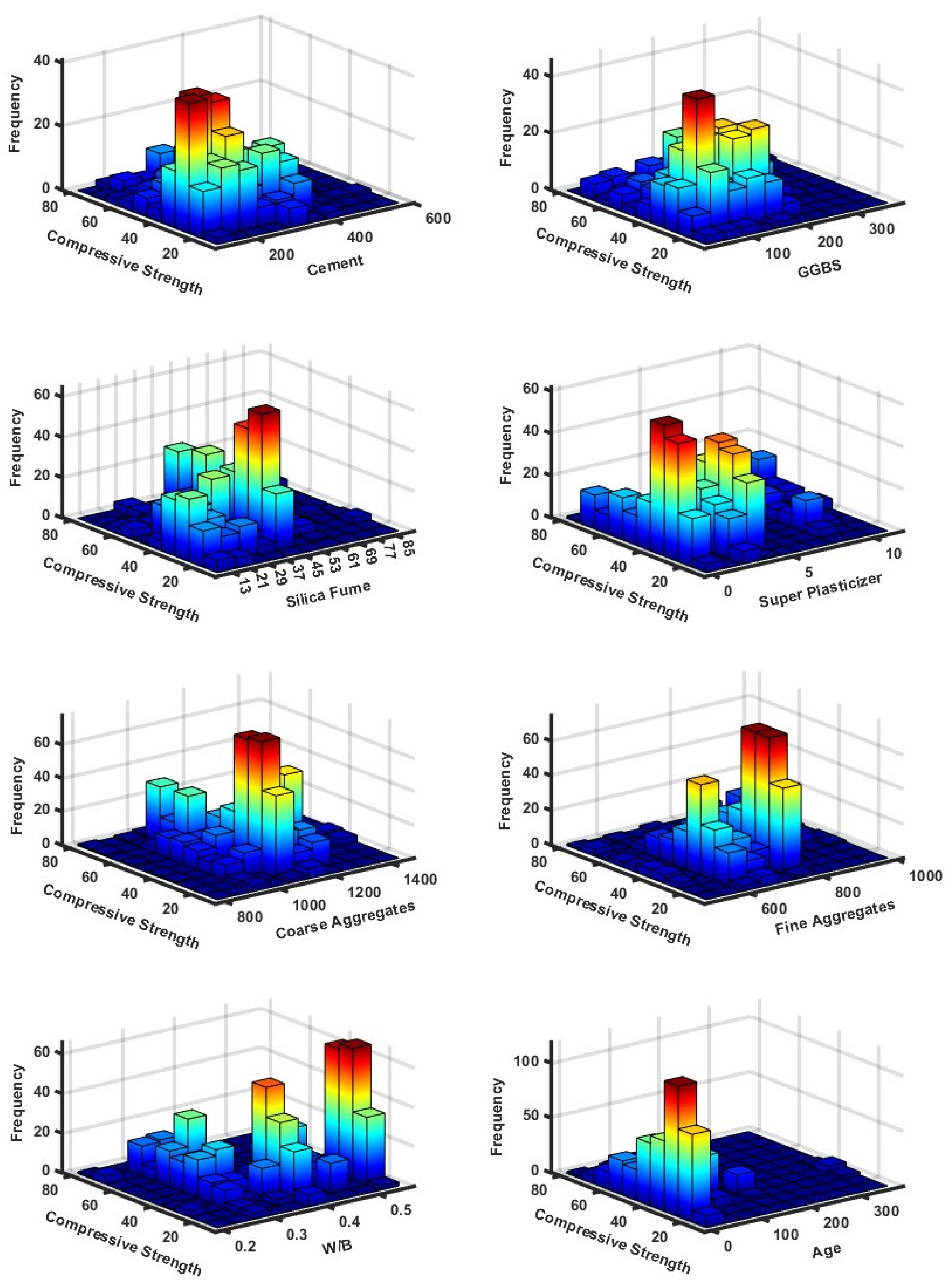
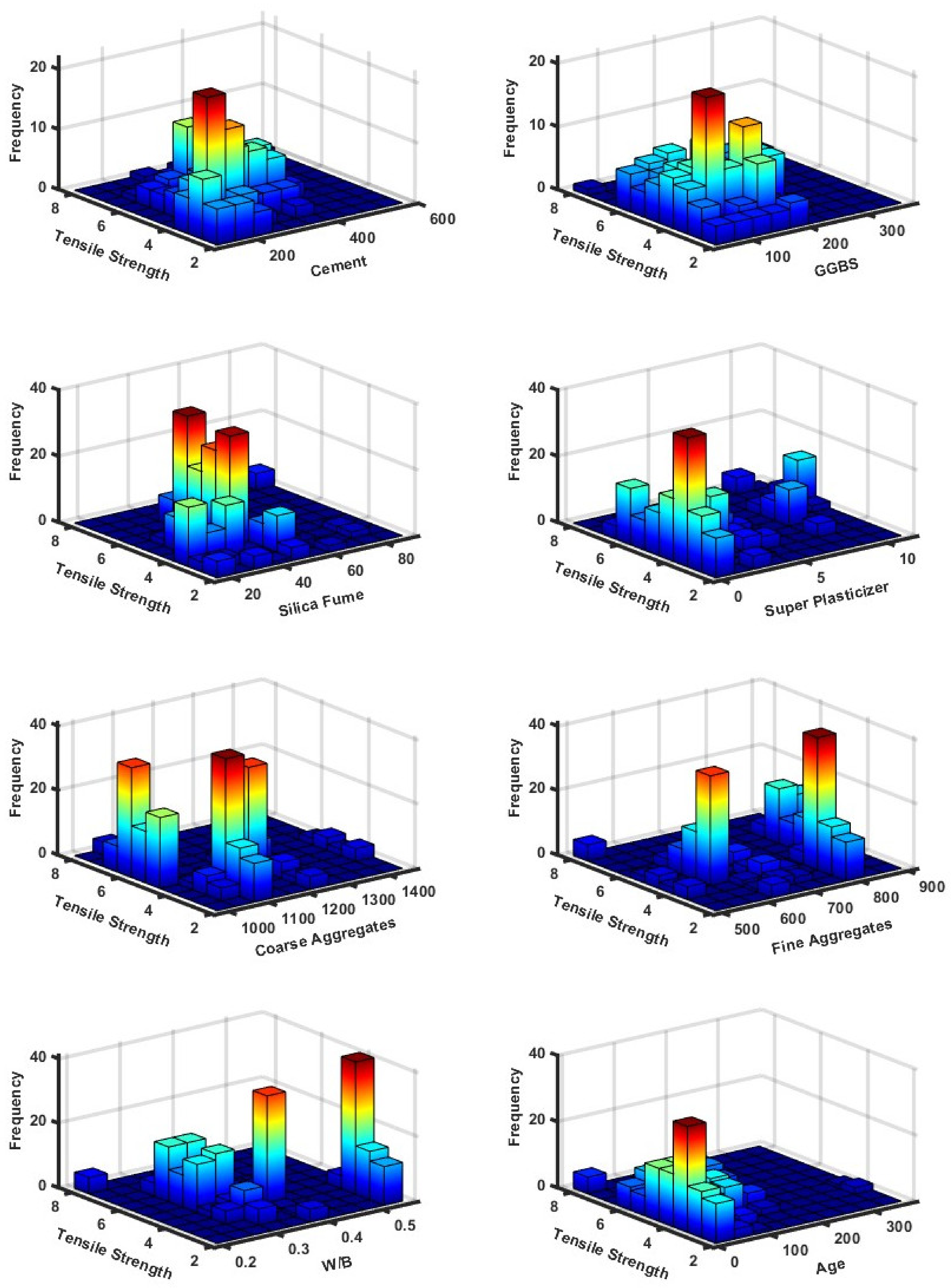
2.1. Data Collection

An extensive database of SCM-based concrete was compiled from articles published in international journals [39,40,41,42,43,44,45,46,47,48,49,50,51,52,53,54,55,56,57,58,59,60,61,62]. The collected database was mainly obtained from concrete mixes incorporated with a combination of SCMs (SF and GGBS). While developing the database, care was taken to select the data points that provided comprehensive details regarding the mix design and sizes of the specimens used. The total dataset consisted of 648 data points for CS and 245 data points for TS. The database comprised two types of concrete samples, i.e., cylinders and cubes. The reported database for CS contains 248 data points obtained from cubic specimens with a size of 150 mm and 400 data points obtained from standard-size cylindrical samples (150 mm in diameter and 300 mm in height). However, according to previous experimental investigations, the length-to-diameter ratio (L/D) affects the strength properties of concrete [63]. Therefore, for the sake of homogeneity, all of the data points were normalized in standard cylindrical form. A normalization factor of 0.8 was used for the cubes of 150 mm in size [64]. Similarly, the collected database for TS contains 245 data points obtained from standard-size cylindrical specimens. In this study, eight major input parameters, including the water-to-binder ratio (W/B), ground granulated blast furnace slag (GGBS) content, cement content (C), silica fume (SF) content, superplasticizer (SP), specimen age (A), and coarse aggregate (CA) and fine aggregate (FA) proportions, were considered to develop the database, while CS and TS were used as output parameters. It is known that the distribution of the input data of any model has a significant impact on its performance [65]. Before developing the models, it is important to ensure that the data are randomly distributed without biasness, and outliers should be detected. This study used the raincloud visualization technique with a normal distribution curve to determine potential outliers in the database, as shown in Figure 3 and Figure 4 for CS and TS, respectively. It can be noted that only a few data points deviated from the normal trend. Several statistical techniques could be used to eliminate the effect of outliers, such as data trimming, imputation, and data transformation [66]. The selection of the most appropriate outlier detection technique depends on the type of data. The imputation technique can be considered the most effective outlier detection method when the data slightly deviate from the normal trend [67]. Therefore, this study also employs an imputation technique in which the outliers are replaced with mean values. After the outlier analysis, the distribution of input parameters and their relationship with the performance indicators (CS and TS) are calculated, as shown in Figure 5 and Figure 6, respectively. It is evident that the input data are distributed randomly without any biasness.

For analysis, the whole database was split into three categories, i.e., training, validation, and testing subsets. The training database was used for the general evolution of the model, while the validation and testing databases were utilized to assess the model’s predictive validity. When partitioning a dataset into categories, it is crucial to make sure that the data distribution is uniform in the training and validation phases. This objective was accomplished through the random arrangement of the training (learning), validation, and testing (evaluation) datasets, ensuring that the variables being used exhibited a satisfactory level of consistency with regard to statistical properties, including the mean, median, and standard deviation, as well as the range of data. The present study employed a training dataset comprising 70% of the total data for both CS and TS (454 and 171 data points), while the remaining 30% of the total data points (194 and 74) were allocated to validate the models. Before running the models, numerous tests were performed to evaluate whether the consistency of the database was valid.

The statistical analyses of input parameters used for CS and TS models are given in

Table 1. Statistical description of the CS parameters.

Parameters		Minimum	Mean	Range	Median	Kurtosis	Mode	SD	Skewness	Maximum
Inputs	Units
C	kg/m3	113.4	254.0	463.6	243.0	−0.3	270.0	87.9	0.5	577.0
GGBS	kg/m3	21.5	126.2	348.5	129.6	−0.1	64.8	57.6	0.5	370.0
SF	kg/m3	9.0	36.1	80.0	38.7	0.9	45.0	15.0	0.5	89.0
SP	kg/m3	0.0	3.1	11.3	3.8	0.6	0.0	3.1	1.0	11.3
CA	kg/m3	793.0	1090.8	655.0	1093.0	4.0	1093.0	91.7	1.2	1448.0
FA	kg/m3	499.0	724.9	493.0	768.0	−0.5	785.0	98.5	−0.2	992.0
W/B		0.2	0.4	0.4	0.4	−1.2	0.6	0.1	0.2	0.6
Age	Days	1.0	50.8	364.0	28.0	9.8	28.0	63.0	2.8	365.0
Output
CS	MPa	11.2	39.2	69.6	35.2	−0.2	34.4	14.3	0.7	80.8

and

Table 2. Statistical description of the TS parameters.

Parameters		Minimum	Mean	Range	Median	Kurtosis	Mode	SD	Skewness	Maximum
Inputs	Units
C	kg/m3	113.4	261.4	463.6	270.0	0.0	270.0	83.6	0.4	577.0
GGBS	kg/m3	45.0	135.8	325.0	135.0	0.0	45.0	58.4	0.4	370.0
SF	kg/m3	16.2	40.3	72.8	45.0	2.4	45.0	13.9	0.6	89.0
SP	kg/m3	0.0	2.8	11.3	0.0	−0.1	0.0	3.8	1.1	11.3
CA	kg/m3	985.0	1108.5	463.0	1093.0	2.0	1093.0	108.1	1.3	1448.0
FA	kg/m3	499.0	723.5	401.0	785.0	−1.1	785.0	114.3	−0.3	900.0
W/B		0.2	0.4	0.4	0.4	−1.3	0.6	0.1	0.5	0.6
Age	Days	7.0	68.5	358.0	56.0	5.1	28.0	62.2	1.9	365.0
Output
TS	MPa	2.1	4.5	6.1	4.3	−0.1	3.7	1.2	0.5	8.3

, respectively. These provide details about the standard deviation, mode, kurtosis, median, skewness, range, smallest, and highest values of the datasets being used for both CS and TS models. A minimal standard deviation value demonstrates that most values are concentrated in a very narrow range around the mean value in the normal distribution curve. On the other hand, a higher standard deviation shows that the numbers are dispersed more widely. The skewness of a variable is the degree to which the distribution of its probabilities deviates from symmetry with respect to the mean [68]. According to Brown and Greene [69], the acceptable kurtosis value is within the range of −10 to +10, and this value indicates the type of probability distribution. The abovementioned statistical measures show that the data are distributed over a wider range, making the models more generalized. Moreover, the efficacy of the model can be enhanced by the distribution of input variables across a wide range. It is essential to carefully examine the mutual dependency of specific parameters utilized in model construction to avoid complexity in the analysis of the model’s results. The issue of correlation among particular variables is commonly known as multi-collinearity. To avoid this concern, it is recommended that the correlation coefficient between the two variables should be lower than 0.8 [70].

Table 3. Correlation coefficient metrics for the CS parameters.

	C	GGBS	SF	SP	CA	FA	W/B	Age	CS
C	1
GGBS	−0.2172	1
SF	0.0304	0.1853	1
SP	−0.0681	0.0145	0.2537	1
CA	−0.0004	−0.0160	−0.1282	−0.0553	1
FA	−0.4142	−0.1128	0.0059	0.3206	−0.5484	1
W/B	−0.5972	−0.2312	−0.2535	−0.2416	0.1206	0.3244	1
Age	−0.1608	−0.0225	0.0425	0.0707	−0.0420	0.1705	0.1828	1
CS	0.2388	0.2360	0.2262	0.2561	−0.3149	0.2068	−0.5637	0.2442	1

and

Table 4. Correlation coefficient metrics for the TS parameters.

	C	GGBS	SF	SP	CA	FA	W/B	Age	TS
C	1
GGBS	−0.2450	1
SF	0.3150	0.1287	1
SP	0.1128	0.1204	0.2327	1
CA	−0.0548	0.1256	−0.3269	−0.0927	1
FA	−0.3015	−0.2016	−0.0832	0.2561	−0.6536	1
W/B	−0.6520	−0.2686	−0.3952	−0.4985	0.0654	0.2200	1
Age	0.0304	−0.0619	0.0519	0.1025	−0.1778	0.1123	−0.0198	1
TS	0.5449	0.1457	0.4139	0.5142	−0.3211	0.0702	−0.7511	0.3124	1

indicate that all variables utilized in the model exhibit a weak correlation, as indicated by both the negative and positive correlation values.

2.2. Overview of Soft Computing Techniques

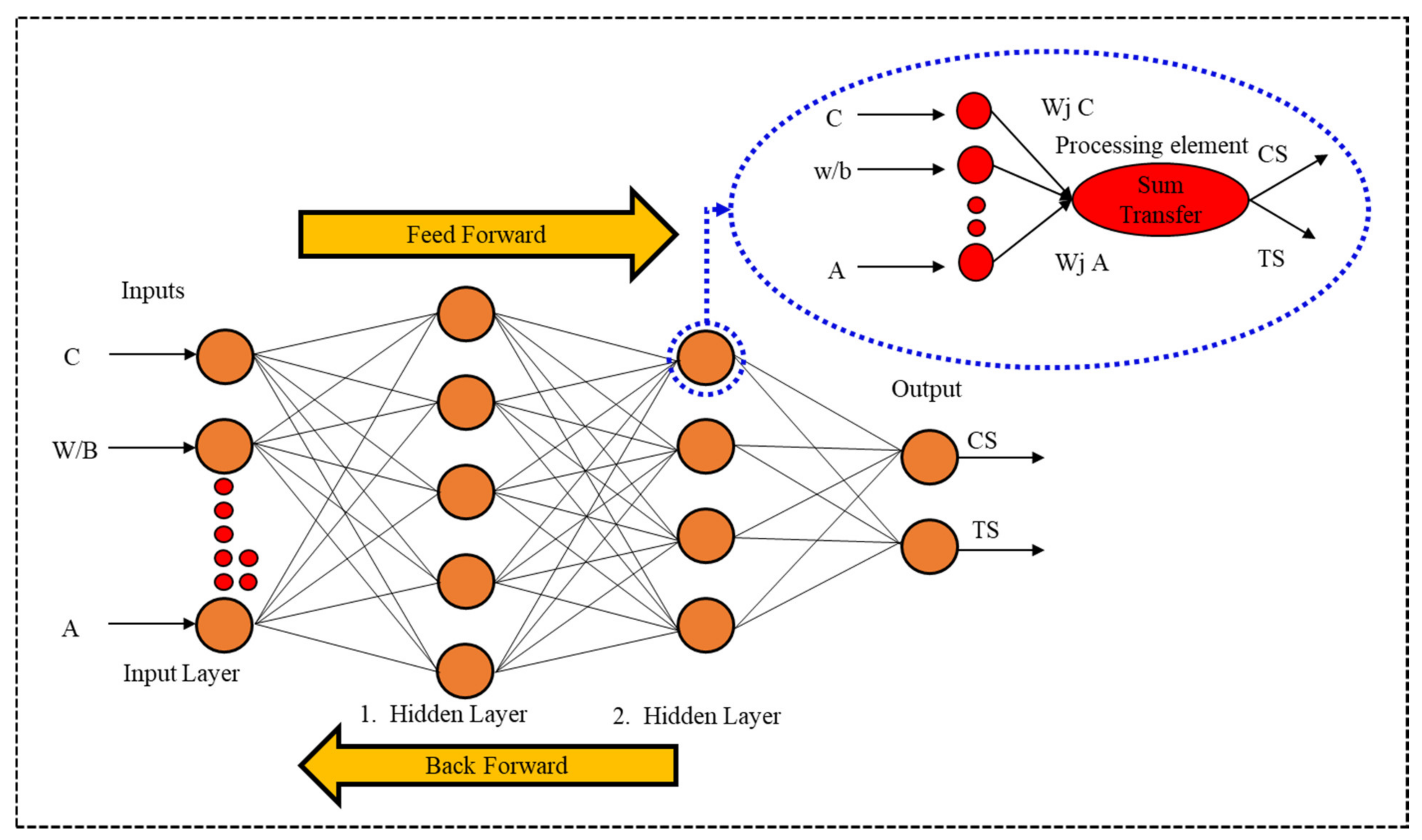
2.2.1. Artificial Neural Networks

Artificial Neural Networks (ANNs), initially introduced by McCulloch et al. [71], are computational models utilized for the efficient prediction and categorization of non-linear regression problems. Neural networks comprise fundamental computational elements known as neurons, which are grouped into layers. Every single neuron in a particular layer is linked to all of the neurons in the adjacent layer. The computational structure is structured hierarchically, with at least three layers comprising its composition: the input layer (input neurons), one or more computational layers (hidden layers), and the output layer, as demonstrated in Figure 7. The input layer is accountable for acquiring variables for the training and evaluation of the model. Likewise, the computational layer is accountable for linking the input and output layers to help with the processing of data, which are subsequently transmitted to the output layer to generate the model’s outcomes [72]. This study employs the process of forward propagation, which is accomplished through a sequential pathway in which the preceding neuron receives and interprets data before transmitting the data to the succeeding neurons. Simultaneously, every input is subjected to the influence of weight (Wj w/b, Wj C, Wj GGBS, Wj SF, Wj SP, Wj A, Wj CA, Wj FA), which denotes the varying degrees of the significance of the input data in relation to the output. A threshold value, denoted by j, is added by each node to the sum of weighted signal inputs.

Subsequently, a non-linear conversion function is applied to the integrated input (Ij) that transforms a value from one unit of measurement to another. The activation functions (AFs) play a crucial role in ANNs and have a notable impact on the efficacy of the models by introducing non-linearity to the networks. Therefore, selecting an appropriate AF is a critical consideration [73]. Several commonly utilized AFs for improving the efficacy of ANN models have been identified in the literature [74,75]. The activation conversion functions that are frequently employed in artificial neural networks (ANNs) include logistic sigmoid, linear, and hyperbolic tangent sigmoid functions [76]. The present study employed a linear transfer function (PURELIN) and a BPNN transfer function (TRANSIG). These functions result in an increased statistical performance and number of neurons in the training phase, while decreasing the performance accuracy in the testing and confirmation phases [77]. The logistic function, which is represented by Equation (1), was employed as an AF in this study. The ANN method is mathematically represented by Equations (1)–(3).

$${\mathrm{z}}_{\mathrm{h}}\left(\mathrm{x}\right)=\frac{1}{1+{\mathrm{e}}^{-\mathrm{x}}}$$

(1)

$${\mathrm{I}}_{\mathrm{j}}=\left\{\left({\mathrm{w}}_{\mathrm{j} \mathrm{C}}\ast \mathrm{C}+{\mathrm{w}}_{\mathrm{j} \frac{\mathrm{w}}{\mathrm{b}}}\ast \frac{\mathrm{w}}{\mathrm{b}}+\dots {\mathrm{w}}_{\mathrm{j} \mathrm{A}}\ast \mathrm{A}\right)\right\}+{ \mathsf{\theta }}_{\mathrm{j}} \mathrm{Summation}$$

(2)

$${\mathrm{CS}}_{\mathrm{j}}{ \mathrm{or} \mathrm{TS}}_{\mathrm{j}}=\mathrm{x}\left({\mathrm{I}}_{\mathrm{j}}\right) \mathrm{Transfer}$$

(3)

The training process of an ANN starts with the propagation of data from the input neurons, while the weights are established according to predetermined rules to produce outputs with minimal error. Following that, the model that has undergone training is subjected to scrutiny and validation through a distinct subset of data designated for testing purposes. Further details regarding the ANN modeling methodology can be found in [78].

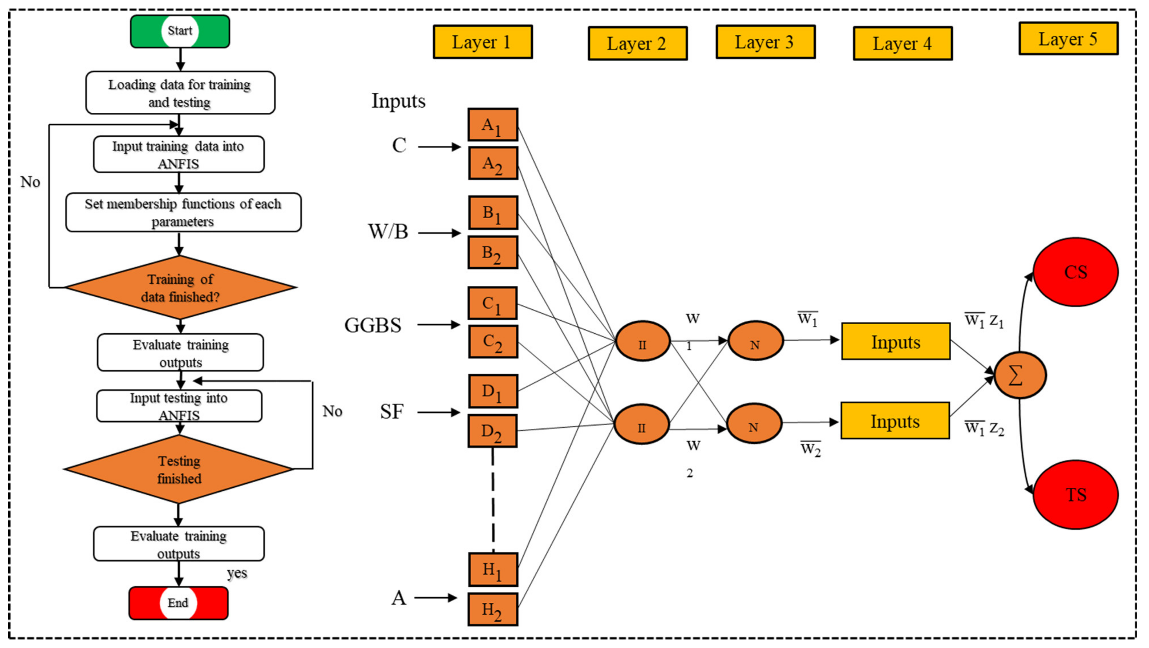
2.2.2. Adaptive Neuro-Fuzzy Inference System (ANFIS)

The ANFIS is an ML model that integrates the features of both fuzzy logic and neural networks. It exhibits superior predictive capabilities and represents a more viable option for computing complex non-linear problems with enhanced accuracy [79]. An ANFIS learns from a training set to construct a fuzzy inference system that can be fine-tuned and optimized through a learning algorithm, similar to the training process of neural networks.

The ANFIS uses a collection of fuzzy if–then regulations to estimate the input–output correlation. The aforementioned regulations are commonly derived from specialized expertise or acquired through a process of learning. In the present study, the fuzzy logic toolbox in the MATLAB R2022a environment was used for the development of ANFIS models. The fuzzy logic toolbox provides a range of functions and tools for the creation of ANFIS models. This toolbox also facilitates the process of training and optimizing the ANFIS model by utilizing the provided data and parameters. The ANFIS comprises multiple layers, wherein the parameters of each layer undergo modifications through the learning process. The initial stage of a fuzzy system involves the acquisition of input variables by the input layer. These variables are subsequently subjected to a fuzzification process in the fuzzification layer, wherein they are converted into fuzzy sets by utilizing membership functions (MFs). Fuzzy if–then rules are utilized in the rule layer to combine the fuzzified inputs. The normalization layer combines the normalized outputs generated by the rule layer, thereby ensuring consistency across the rules. Ultimately, the defuzzification layer transforms the normalized outputs into precise numerical values. During the training process, the fuzzy rules and MF parameters are adapted using a learning algorithm to minimize the differences between the anticipated and actual outputs. This approach aims to optimize the performance of the model. Figure 8 illustrates the ANFIS structure for multiple input variables, wherein the fixed and adaptive nodes are represented by circles and squares, respectively. The ANFIS architecture can be represented by the first order of the Sugeno model, which employs two sets of if–then rules.

Rule 1 applies if C and W/B are A₁ and B₂, respectively.

Then, Equation (4) indicates that

$${\mathrm{z}}_1={\mathrm{p}}_1\left(\mathrm{C}\right)+{\mathrm{q}}_1\left(\frac{\mathrm{w}}{\mathrm{b}}\right)+{\mathrm{r}}_1$$

(4)

Rule 2 applies if C and w/b are A₂ and B₂, respectively.

Then, Equation (5) says that

$${\mathrm{z}}_2={\mathrm{p}}_2\left(\mathrm{C}\right)+{\mathrm{q}}_2\left(\frac{\mathrm{w}}{\mathrm{b}}\right)+{\mathrm{r}}_2$$

(5)

Here,

• A_n and B_n = fuzzy logic sets;
• P_n, q_n, and r_n = shape factors (estimated in the training phase);
• z₁ and z₂ = outputs (CS and TS).

The ANFIS model is composed of five distinct layers, as noted by Golafshani et al. [80]. A comprehensive explanation of the functions of these layers is provided herein.

First Layer: This layer is also known as the fuzzification layer, in which each input variable is fuzzified or converted into a fuzzy set using membership functions.

Equations (6) and (7) represent the basic fuzzy rule and the model parameters, respectively.

$${\mathrm{O}}_{\mathrm{i}}^1={\mathsf{\mu }}_{\mathrm{Ai}}\left(\mathrm{C}\right),\hspace{1em}\hspace{1em} \mathrm{i}=1, 2$$

(6)

$${\mathrm{O}}_{\mathrm{i}}^1={\mathsf{\mu }}_{\mathrm{Bi}-2}\left(\mathrm{w}/\mathrm{b}\right),\hspace{1em}\hspace{1em} \mathrm{i}=3, 4$$

(7)

Here, u is the significance (weight) calculated by linking the fuzzy association function, and both A_i (C) and B_i−2 work together to distinguish one method of applying a fuzzy MF from another. The bell-shaped and gaussian MFs are represented in Equations (8) and (9).

$${\mathsf{\mu }}_{\mathrm{Ai}}\left(\mathrm{C}\right)={\mathrm{e}}^{-\frac{{\left(\mathrm{C}-{\mathrm{c}}_{\mathrm{i}}\right)}^2}{2{{\mathrm{a}}_{\mathrm{i}}}^2}}$$

(8)

$${\mathsf{\mu }}_{\mathrm{Ai}}\left(\mathrm{C}\right)=\frac{1}{1+{\left\{\left(\frac{\mathrm{C}-{\mathrm{c}}_{\mathrm{i}}}{{\mathrm{a}}_{\mathrm{i}}}\right)\right\}}^{{\mathrm{b}}_{\mathrm{i}}}}$$

(9)

Second Layer: The resulting response of this layer relates to the firing capacity of the pre-specified regulations applied to a given input series. The points in the second layer are fixed and execute basic multiplication operations. The resulting output boundaries are presented in Equation (10).

$${\mathrm{O}}_{\mathrm{i}}^2={\mathrm{w}}_{\mathrm{i}}={\mathsf{\mu }}_{\mathrm{Ai}}\left(\mathrm{C}\right)·{ \mathsf{\mu }}_{\mathrm{Bi}}\left(\frac{\mathrm{w}}{\mathrm{b}}\right),\hspace{1em} \mathrm{i}=1, 2$$

(10)

Third Layer: In this layer, the outputs obtained from the second layer are normalized to ensure that the overall output is within a specified range. This step is important for consistency and comparability across different rules. Layer outputs are illustrated in Equation (11).

$${\mathrm{O}}_{\mathrm{i}}^3=\overline{{\mathrm{w}}_{\mathrm{i}}}=\frac{{\mathrm{w}}_{\mathrm{i}}}{{\mathrm{w}}_1+{\mathrm{w}}_2}\hspace{1em} \mathrm{i}=1, 2$$

(11)

Fourth Layer: In the fourth layer, the nodes exhibit adaptability, and their outcomes are represented as the result of standardized firing strength in conjunction with a first-order polynomial while considering the first-order Sugeno model. Consequently, the resulting output is expressed as Equation (12):

$${\mathrm{O}}_{\mathrm{i}}^3=\overline{{\mathrm{w}}_{\mathrm{i}}}{\mathrm{z}}_{\mathrm{i}}=\overline{{\mathrm{w}}_{\mathrm{i}}}\left\{\left({\mathrm{p}}_{\mathrm{i}}\left(\mathrm{C}\right)+{\mathrm{q}}_{\mathrm{i}}\left(\mathrm{w}/\mathrm{b}\right)+{\mathrm{r}}_{\mathrm{i}}\right)\right\}$$

(12)

Fifth Layer: In the fifth layer, only one permanent node is denoted by the symbol Ʃ. This node is responsible for performing the sum of the weighted consequences of the rules that previously resulted from the previous layer. Consequently, the findings of the model can be obtained by utilizing Equation (13).

$${\mathrm{O}}^5={\sum }_{\mathrm{i}=1}^2\overline{{\mathrm{w}}_{\mathrm{i}}}{\mathrm{z}}_{\mathrm{i}}=\frac{{\sum }_{\mathrm{i}=1}^2\overline{{\mathrm{w}}_{\mathrm{i}}}{\mathrm{z}}_{\mathrm{i}}}{{\mathrm{w}}_1+{\mathrm{w}}_2}$$

(13)

Notably, within the ANFIS framework, only the first and fourth layers exhibit the ability to adapt. The premise parameters, denoted as {a_i, b_i, c_i}, are linked to the input association functions within the first layer of the system. Similarly, the three consequent parameters {p_i, q_i, r_i} are associated with first-order polynomials and are located in the fourth layer, as reported by Islam et al. [81].

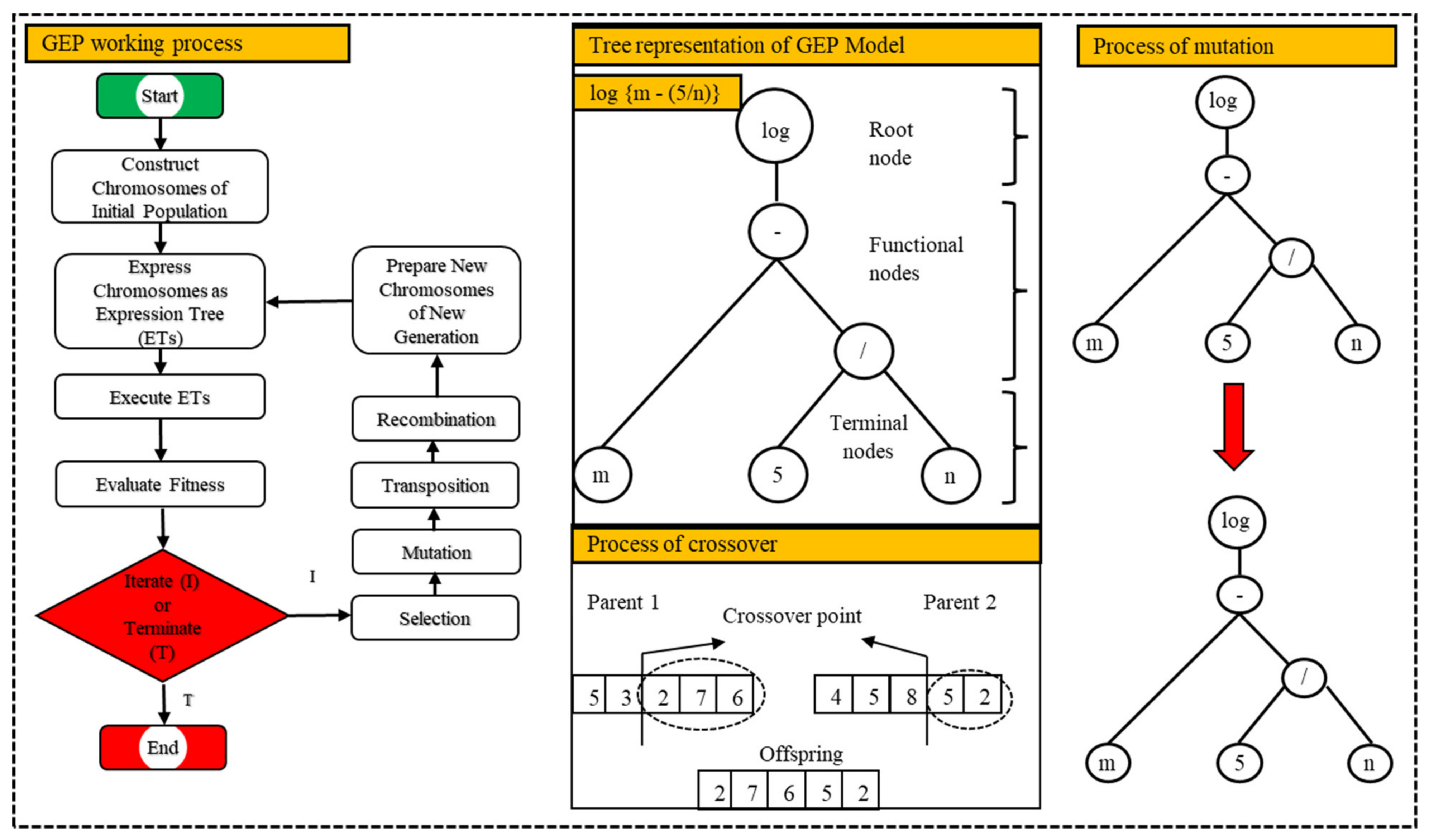
2.2.3. Gene Expression Programming (GEP)

GEP, introduced by Ferrira [82], is a modification of genetic programming (GP) and is premised on the evolutionary population hypothesis. It encompasses simple, fixed-length linear structures like chromosomes, and more complex, non-linear structures like parse trees. The essential parameters that must be specified in GEP are identical to those used in GP, such as the function set, set of terminals, fitness trial, governing parameters, and terminal conditions. Figure 9 shows a graphical description of the GEP working procedure. Chromosomes of fixed length are first generated at random for each individual gene. Static-length linear strings are then represented as non-linear structures of various sizes and form termed expression trees (ETs), indicating chromosomes of branched structures [83]. It is important to mention that in GEP, genotypes (genetic constitution) and phenotypes are separated so that the program can benefit from all of evolution’s merits [82]. Then, each individual’s fitness is assessed by expressing the chromosomes as ETs. For use in the reproduction phase, the best-fit individuals are chosen. The iterations are repeated with new individuals in search of the optimal solution. Several genetic operations like crossover, mutations, and reproduction are executed for the transformation of populations. Figure 9 shows the ET representations of the GEP model and the crossover and mutation processes. The notable modification in GEP is that the genome (haploid set of chromosomes) is passed down to the succeeding generation, and the whole structure does not need to be replicated and transformed because all modifications occur in a perfectly linear framework. Another important characteristic to note is that every individual is composed of a single chromosome containing several genes, which are then separated into head and tail segments [83]. Additionally, genetic algorithms are used to change chromosomes during the reproductive stage [84]. Finally, GEP models can modify the parameter arrangement based on how well it fits with the results of the experiments.

2.3. Model Structures

Before developing a model, the first step is creating a general function. The input parameters that have the most significant effect on the properties of concrete were selected in this function, and parameters having a negligible influence on the properties of concrete were neglected. As a result, the following variables were found to be functions of the mechanical characteristics of concrete incorporated with SF and GGBS:

$$\mathrm{CS} \mathrm{and} \mathrm{TS} \left(\mathrm{MPa}\right)=\mathrm{f}\left(\mathrm{C},\mathrm{GGBS},\mathrm{SF},\mathrm{SP},\mathrm{CA},\mathrm{FA},\frac{\mathrm{W}}{\mathrm{B}},\mathrm{A}\right)$$

(14)

The ANN models were developed by using the Levenberg–Marquardt method. The data were portioned randomly, and a total of 10 hidden neurons were used. The feed-forward back-propagation network type was employed for the iteration process. It is crucial to note that, in this study, the trial-and-error method was adapted to achieve optimal performance concerning the desired number of hidden layers [28].

Table 5. Parametric settings for training the ANN models.

Parameter Type	Value/Type
Data Distribution	CS	TS
Total dataset	682	245
Calibration (training) (70%)	454	171
Testing (15%)	97	37
Validation (15%)	97	37
General settings
Hidden neurons	10
Network type	Feed-forward back-propagation
Output layer transfer function	PURELIN
Training method	Levenberg–Marquardt
Computational layer transfer function	TANSIG
Epochs	41
Data division	Random
Rate of learning	0.01
Non-linear parameters	18

presents the statistical parameters used for the modeling process using the ANN approach in the present study.

The ANFIS exhibits constraint when accommodating a single output compared to an ANN. Hence, the outputs were subjected to independent treatment, with identical input variables being considered for both the ANN and ANFIS models. Similar datasets of training, testing, and validation were used for ANFIS modeling to observe the optimized outcomes. Initially, the hybrid optimization method, specifically the least-square and back-propagation method, was employed to generate the fuzzy inference system (FIS) using subtractive clustering, also known as “sub-clustering”. Subsequently, the FIS was trained utilizing the trim function, as documented by Jalal et al. [85]. It is important to emphasize that this approach was used due to the extensive database. Moreover, Venkatesh and Bind [86] suggested using the grid portioning technique in cases where the total amount of inputs is six or fewer. In this study, trial-and-error methods were adapted, the ANFIS model was trained, and optimal parameter values were determined using an initial number of epochs as 40. The term “epoch” refers to the number of iterations or passes over the training set that the program was allowed to run. Each epoch represents a complete iteration through the training data.

Table 6. Parametric settings for training the ANFIS models.

Parameter Type	Value/Type
Data Distribution	CS	TS
Total dataset	648	245
Calibration (training) (70%)	454	171
Testing (15%)	97	37
Validation (15%)	97	37
General settings
Number of nodes	10	10
Number of fuzzy rules	7	8
Number of non-linear parameters	50	77
Epochs	40	40
Number of linear parameters	66	120
Number of MFs	18	89
Error goal in training	0	0
Fuzzy structure	Sugeno
Output function	Linear
Optimization technique	Hybrid method
MF type	trimf
FIS type	Sub-clustering

presents a comprehensive list of the different setting parameters used to train the ANFIS models.

In the process of developing the GEP models for the anticipation of the CS and TS of concrete containing SF and GGBS, GeneXproTools 5.0, a highly adaptable GEP data modeling program, was used. This is a user-friendly and effective data mining tool created specifically for categorization, time-series analysis, basic functional regression, and logical synthesis. A well-structured Microsoft Excel (v2010) dataset with eight input parameters and established outputs was uploaded to begin the simulation process.

The generalization capability and robustness of the generated model greatly depend on its fitting parameters. Initially, numeric constants and genetic operators were chosen based on the literature, and 20 trial-and-error-based models were run for each output (CS and TS) to determine the best settings. Different fitting parameter combinations were used by varying the gene number, head size, number of genetic factors (chromosomes), and linking functions [22]. The operating time of each model was determined according to the number of genetic factors. The basic genetic operators and numeric constants utilized for both the CS and TS predictive models are explained in

Table 7. Genetic operators and numeric constants used in the GEP models for CS and TS.

Genetic Operators
RIS transposition rate	0.00541
Permutation	0.00546
Two-point recombination rate	0.00273
Leaf mutation	0.00546
Gene recombination rate	0.00274
Conservative mutation	0.00364
Rate of gene transposition	0.00272
Mutation	0.00138
Rate of mutation	0.00134
Fixed-root mutation	0.00182
Rate of inversion	0.00535
IS transposition rate	0.00531
Numerical Constants
Data type	Floating number
Method	Random selection
Lower bound	−10
Fine-tuning	0.0026
Constant per gene	10
Upper bound	10

. The fitness parameters employed in each of the 20 GEP models for CS are listed in

Table 8. Descriptive summary of the parametric settings of the GEP models used for CS.

Models	No. of Chromosomes	Variable Used	Head Size	Constant per Genes	Number of Genes	Linking Function	Ftn Set	Duration (Minutes)
CS1	30	7	8	10	3	Addition	(÷, ×, +, −)	20
CS2	50	7	10	10	4			23
CS3	80	9	12	10	5			25
CS4	100	7	14	10	6			30
CS5	150	7	16	10	7			40
CS6	30	7	8	10	3	Division	(÷, ×, +, −)	23
CS7	50	9	10	10	4			26
CS8	80	9	12	10	5			29
CS9	100	8	14	10	6			35
CS10	150	7	16	10	7			45
CS11	30	9	8	10	3	Multiplication	(÷, ×, +, −)	18
CS12	50	8	10	10	4			22
CS13	80	9	12	10	5			24
CS14	100	8	14	10	6			27
CS15	150	8	16	10	7			35
CS16	30	7	8	10	3	Multiplication	(÷, ×, +, −, Pow, √)	30
CS17	50	9	10	10	4			34
CS18	80	8	12	10	5			38
CS19	100	9	14	10	6			42
CS20	150	8	16	10	7			50

, and for the TS models, these parameters are listed in

Table 9. Descriptive summary of the parametric settings of the GEP models used for TS.

Models	No. of Chromosome	Variable Used	Head Size	Constant per Genes	Number of Genes	Linking Function	Function Set	Duration (Minutes)
TS1	30	7	8	10	3	Addition	(÷, ×, +, −)	22
TS2	50	8	10	10	4			24
TS3	80	9	12	10	5			26
TS4	100	9	14	10	6			32
TS5	150	9	16	10	7			40
TS6	30	8	8	10	3	Division	(÷, ×, +, −)	24
TS7	50	8	10	10	4			26
TS8	80	7	12	10	5			28
TS9	100	8	14	10	6			33
TS10	150	7	16	10	7			45
TS11	30	9	8	10	3	Multiplication	(÷, ×, +, −)	20
TS12	50	9	10	10	4			22
TS13	80	9	12	10	5			26
TS14	100	8	14	10	6			27
TS15	150	8	16	10	7			37
TS16	30	7	8	10	3	Multiplication	(÷, ×, +, −, Pow, √)	31
TS17	50	7	10	10	4			37
TS18	80	8	12	10	5			38
TS19	100	9	14	10	6			44
TS20	150	9	16	10	7			54

.

2.4. Model Validation

Performance validation is essential to assess the reliability and generalization capability of ML-based models. In this study, statistical metrics and experimental validation criteria were used to assess the efficacy of the proposed models.

2.4.1. Statistical Validation

Initially, the performance of the developed models was evaluated by using statistical error correlations such as the mean absolute error (MAE), relative root-mean-squared error (RRMSE), root mean square error (RMSE), correlation coefficient (R), and root-squared error (RSE). Typically, a model with a higher R² value and lower RMSE, MAE, and RSE values indicates better results. Equations (15)–(20) present the mathematical formulations of these statistical measures.

$$\mathrm{RMSE}=\sqrt{\frac{{\sum }_{\mathrm{i}=1}^{\mathrm{n}}{\left({\mathrm{a}}_{\mathrm{i}}-{\mathrm{m}}_{\mathrm{i}}\right)}^2}{\mathrm{n}}}$$

(15)

$$\mathrm{MAE}=\frac{{\sum }_{\mathrm{i}=1}^{\mathrm{n}}\left|{\mathrm{a}}_{\mathrm{i}}-{\mathrm{m}}_{\mathrm{i}}\right|}{\mathrm{n}}$$

(16)

$$\mathrm{R}=\frac{{\sum }_{\mathrm{i}=1}^{\mathrm{n}}{\left({\mathrm{a}}_{\mathrm{i}}-{\overline{\mathrm{a}}}_{\mathrm{i}}\right)}^2{\left({\mathrm{m}}_{\mathrm{i}}-{\overline{\mathrm{a}}}_{\mathrm{i}}\right)}^2}{\sqrt{{\sum }_{\mathrm{i}=1}^{\mathrm{n}}{\left({\mathrm{a}}_{\mathrm{i}}-{\overline{\mathrm{a}}}_{\mathrm{i}}\right)}^2{\sum }_{\mathrm{i}=1}^{\mathrm{n}}{\left({\mathrm{m}}_{\mathrm{i}}-{\overline{\mathrm{a}}}_{\mathrm{i}}\right)}^2}}$$

(17)

$$\mathrm{RSE}=\frac{{{\displaystyle \sum }}_{\mathrm{i}=1}^{\mathrm{n}}{\left({\mathrm{m}}_{\mathrm{i}}-{\mathrm{a}}_{\mathrm{i}}\right)}^2}{{{\displaystyle \sum }}_{\mathrm{i}=1}^{\mathrm{n}}{\left(\overline{\mathrm{a}}-{\mathrm{a}}_{\mathrm{i}}\right)}^2}$$

(18)

$$\mathrm{RRMSE}=\frac{1}{\left|\overline{\mathrm{a}}\right|}\sqrt{\frac{{{\displaystyle \sum }}_{\mathrm{i}=1}^{\mathrm{n}}{\left({\mathrm{a}}_{\mathrm{i}}-{\mathrm{m}}_{\mathrm{i}}\right)}^2}{\mathrm{n}}}$$

(19)

$$\mathsf{\rho }=\frac{\mathrm{RRMSE}}{\mathrm{R}}$$

(20)

Here, m_i and a_i represent the model and experimental (actual) output values, while ${\overline{\mathrm{a}}}_{\mathrm{i}}$ and ${\overline{\mathrm{a}}}_{\mathrm{i}}$ represent the mean values of the model and experimental outputs, respectively, and n is the total size of the population (database). For an effective and stable correlation between the actual and anticipated values, it has been suggested that it is better to have an R value larger than 0.8 [87]. However, this value was excluded due to its negligence towards the multiplication and division of outcomes to a constant [87]. Therefore, R² was also employed due to its unbiased evaluation and comparatively higher efficiency. The maximum variation among the input parameters is captured when R² values are equal to 1 [88]. There is another statistical correlation commonly used for performance measures, i.e., RMSE. This metric is most prominent because large errors are addressed more efficiently than small errors, and an error value near zero indicates the best model [89]. However, it does not always guarantee the accuracy of identifying the lowest error in prediction. Due to this, the MAE was also estimated, which is very beneficial when dealing with continuous and smooth data [90]. In essence, better and improved models are indicated by lower error statistical metrics (MAE, RSE, and RMSE) and greater R and R² values.

However, a major issue related to AI approaches is overfitting, which results in higher errors in the testing dataset. Hence, minimization of the objective function (OBF) is performed to select the most suitable prediction model, as demonstrated in Equation (8) [65]. The OBF is calculated to assess the trained model’s effectiveness, including error function and changes in the correlation coefficient. The overfitting problem can be fixed by lowering the OBF value.

$$\mathrm{OBF}=\left(\frac{{\mathrm{n}}_{\mathrm{T}}-{\mathrm{n}}_{\mathrm{V}}}{\mathrm{n}}\right){\mathsf{\rho }}_{\mathrm{i} \mathrm{T}}+2\left(\frac{{\mathrm{n}}_{\mathrm{V}}}{\mathrm{n}}\right){\mathsf{\rho }}_{\mathrm{i} \mathrm{V}}$$

(21)

V and T subscripts denote validation and training data points, respectively, and n refers to the total size of the population. A model having an OBF value closer to zero represents the most appropriate model since it comprises the impact of both the RRMSE and R values.

2.4.2. Experimental Validation

Materials

In the present study, OPC Grade53, SF, and GGBS were utilized as cementitious materials in the mixture. The chemical compositions and physical characteristics of these materials are shown in

Table 10. Properties of cementitious materials [91,92].

Component	OPC	GGBS	SF
Chemical Composition (% Mass)
K2O	–	0.69	0.56
CaO	62.73	33.06	0.22
Fe2O3	3.95	0.34	0.5
SO3	3.14	2.67	0.12
SiO2	20.78	35.84	97.5
Na2O	0.78	1.08	0.25
Al2O3	4.82	12.43	0.2
MgO	1.57	12.08	0.56
Physical Properties
Specific gravity	3.15	3.05	2.22
Specific surface area (m2/kg)	421	550	2300
Loss on ignition	2.08	2.08	2.08

. The mineralogical compositions of these cementitious materials can have notable impacts on the properties of concrete, such as its strength, durability, and workability. SF, for instance, is known to enhance the strength and durability of concrete due to its pozzolanic reaction and filler effect. On the other hand, GGBS contributes to improved workability and strength due to filler effects. However, in this study, OPC cement was used for the whole experimental part. Similarly, throughout the experimental investigation, the mineralogical compositions of SF and GGBS remained the same in order to evaluate the specific effects of SF and GGBS on concrete properties when other factors are held constant. River sand and granite with a maximum size of 4.75 mm and 19 mm were used as fine aggregates (FAs) and coarse aggregates (CAs) in the mixtures. The properties of the CAs and FAs were thoroughly examined. The fineness moduli of the FAs and CAs were measured as 2.2 and 5.3, respectively. Likewise, the water absorption and specific gravity were determined as 2.1% and 2.57, and 4% and 3.41, for the FAs and CAs, respectively. In addition, the superplasticizer type S-3 was used to maintain the workability of the concrete samples.

Mix Design and Specimen Preparation

A total of 54 concrete samples, with varying proportions of SF and GGBS, were prepared. The details of the mix designs for external validation are presented in

Table 11. Mix designs used for external validation.

Code	SCMs	Cement	SP	SF	Water	GGBS	CA	FA
		(kg/m3)	(kg/m3)	(kg/m3)	(kg/m3)	(kg/m3)	(kg/m3)	(kg/m3)
CM	CM	415	10	0	156	0	1050	730
M1	SF5+GGBS10	353	10	20	156	41	1050	730
M2	SF10+GGBS20	291	10	41	156	83	1050	730
M3	SF10+GGBS30	249	10	41	156	125	1050	730
M4	SF15+GGBS30	228	10	62	156	125	1050	730
M5	SF20+GGBS40	166	10	83	156	166	1050	730

. In total, six different mixes were designed. CM represents the control mix, while M1 to M5 represent mixes with different percentages of SF and GGBS replacing the cement. The percentage of SF in these mixes varied from 5 to 20, while the percentage of GGBS varied from 10 to 40. For example, M1 represents a mix containing 5 percent SF and 10 percent GGBS as a replacement. As discussed earlier, the main aim of this study is to evaluate the impact of SF and GGBS in concrete; therefore, the W/B ratio, mineralogical compositions of cementitious materials, and other ingredients used in the mixes were kept consistent. The concrete specimens were tested for workability using ASTM C143. Likewise, the CS of the samples was evaluated using the ASTM C39 at the ages of 28, 56, and 90 days.

3. Results and Discussion

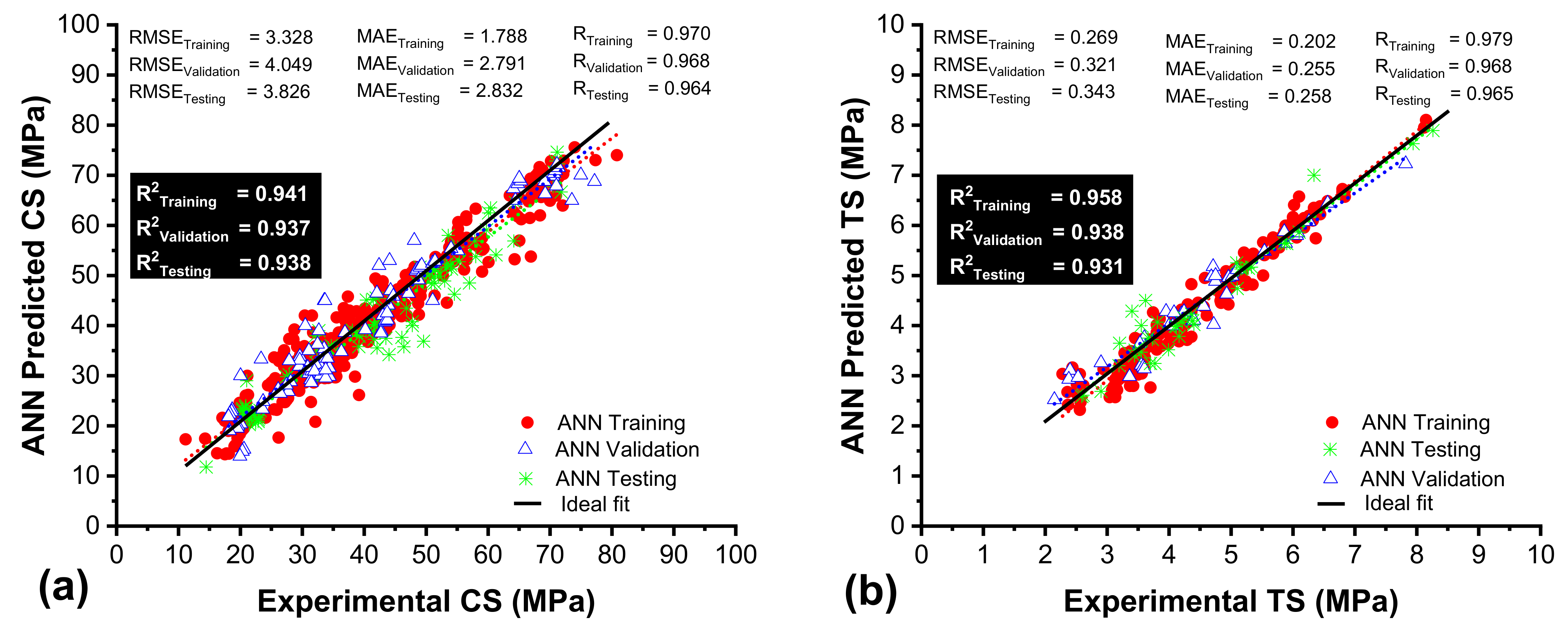
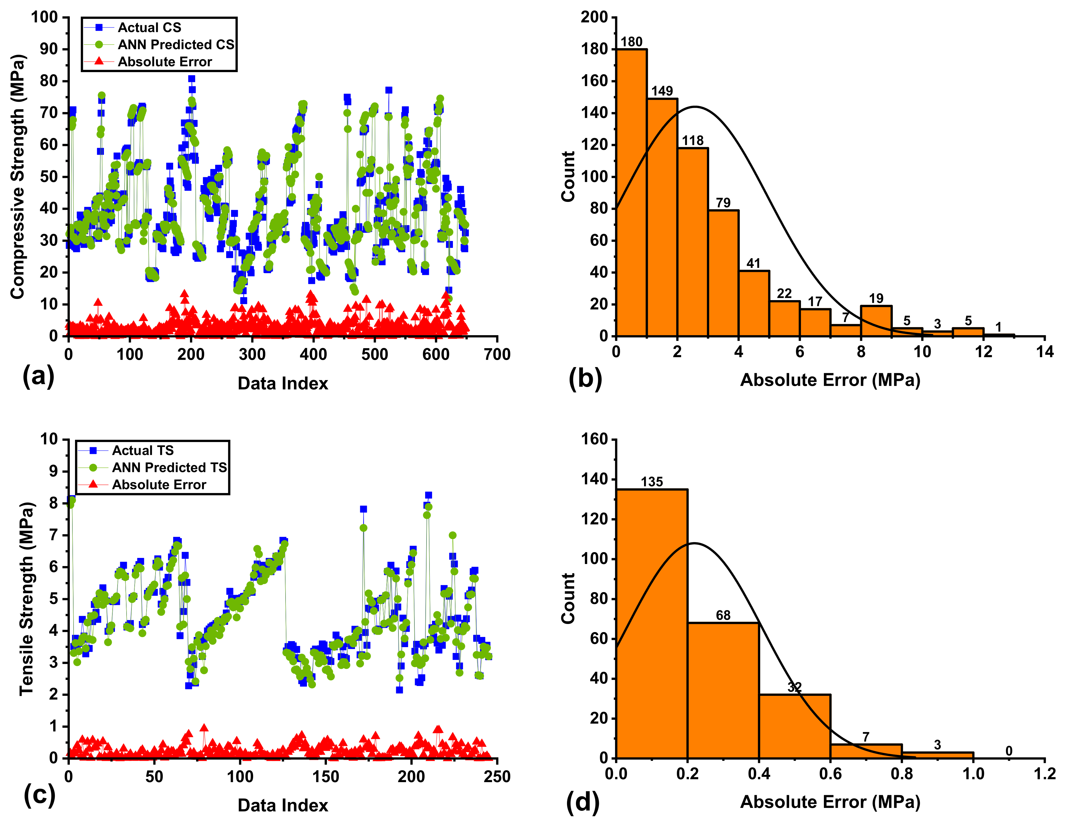
3.1. Performance Assessment of ANN Models

The statistical characteristics and performance index of the training, validation, and testing sets for optimum models of CS and TS based on the ANN models are shown in Figure 10. It is obvious that the R² values for training, validation, and testing for the CS-ANN models are greater than 90% (R²_training = 0.941, R²_validation = 0.937, R²_testing = 0.938). Similarly, for the TS-ANN models, the R² values are 0.958, 0.938, and 0.931 for the training, validation, and evaluation stages, respectively. It is important to mention that the greater difference between the training and validation values is due to the fact that ANN models work on the black-box principle. It can be seen that the error values (RMSE, MAE, RSE, RRMSE) for each set of both CS and TS models are minimal, approaching zero, indicating the higher accuracy of the optimum models. The RMSE values are equal to 3.328 MPa, 4.049 MPa, and 3.826 MPa for the training, validation, and testing phases, respectively, for CS-ANN, and 0.269 MPa, 0.321 MPa and 0.343 MPa for the TS-ANN models. Consequently, the MAE values are equal to 1.788 MPa, 2.791 MPa, and 2.832 MPa for the training, validation, and testing phases of CS-ANN. For the TS-ANN models, these values are 0.202 MPa, 0.255 MPa, and 0.034 MPa, respectively. From these findings, it can be noted that in all three stages for both the CS-ANN and TS-ANN models, the MAE values are lower than RMSE values, indicating a better efficacy of the models. In addition, the PI and OF values for all of the established models in all three stages are close to zero. To further assess the model’s accuracy, the greatest error percentage in the models between the actual and estimated outcomes is depicted in Figure 11a–d. It is evident that the experimental and estimated outcomes are comparable with each other, with maximum errors less than 13 MPa and 0.93 MPa and with means of 2.56 MPa and 0.23 MPa in the CS-ANN and TS-ANN models, respectively. Figure 11b,d illustrates the error histograms for the CS-ANN and TS-ANN models. These figures demonstrate that greater than 81.17% of the projected results lie within the range of 0 to 4 MPa for the employed data in the case of the CS-ANN model. Meanwhile, greater than 90% of the anticipated TS values fall within the error range of 0 MPa to 6 MPa. It is clear from Figure 11 that the error values are closer to zero, which is evidence of the better performance of ANN-based models.

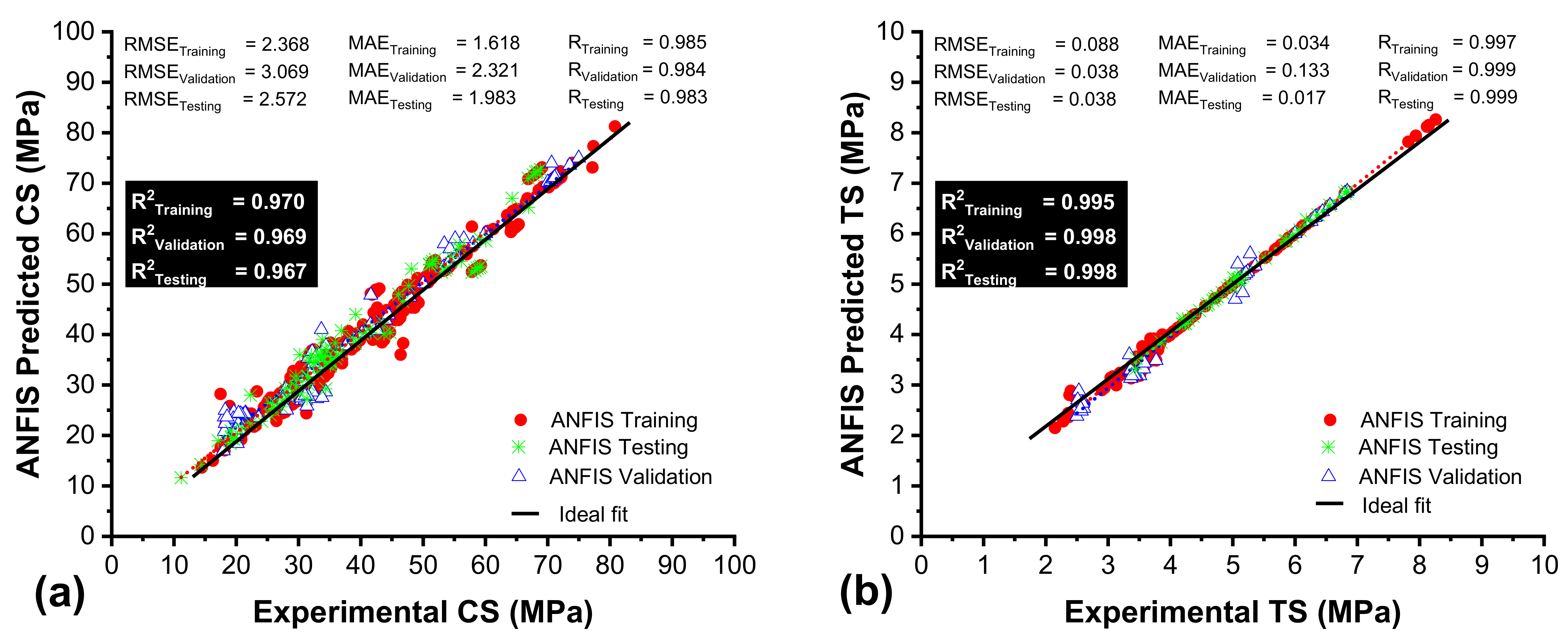
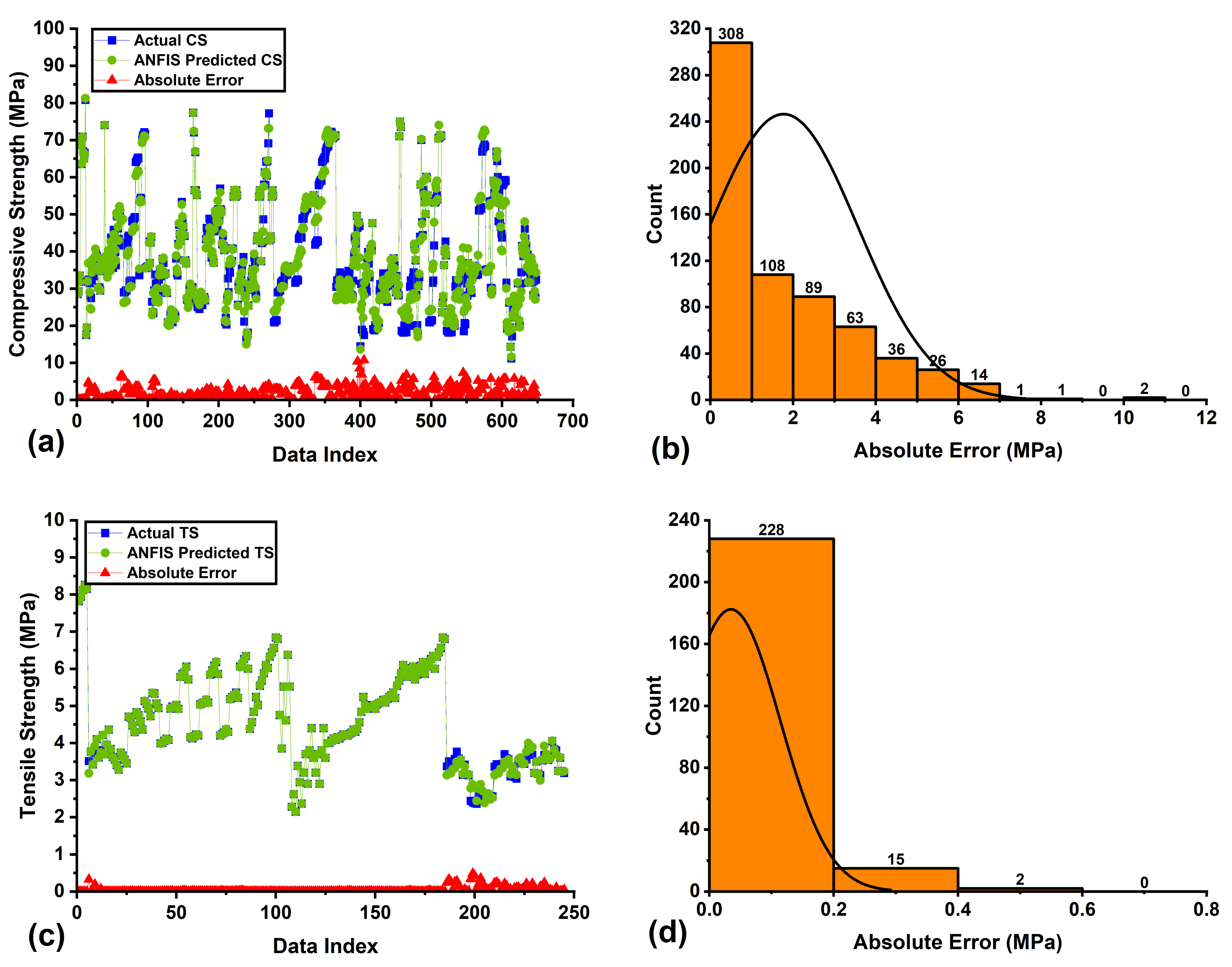
3.2. Performance Assessment of ANFIS Models

In order to enhance efficiency, similar datasets generated by the ANN models were used as input for the ANFIS models. However, a difference was observed between the predictive outcomes of both techniques. This difference can be attributed to the use of additional fuzzy logic in the ANFIS models. It is obvious from Figure 12 that the R² values are 0.97, 0.969, and 0.967 for all three stages, i.e., training, validation, and evaluation (testing), respectively, for the CS-ANFIS models, and 0.995, 0.998, and 0.998 for the TS-ANFIS models. These higher R² values reveal the strong predictive performance of ANFIS-based models. Like ANN-based models, the RMSE and MAE values for the CS-ANFIS and TS-ANFIS models are close to zero, and the MAE values are lower than the RMSE values. Moreover, the ANFIS models show 33% and 30% lower RMSE and MAE values than the ANN models for CS and approximately 85% and 93% lower for TS. Additionally, the RRMSE, OF, and RSE values are close to zero for both the CS-ANFIS and TS-ANFIS models. To determine the predictive performance of ANFIS-based models, the absolute error plots between the ANFIS-anticipated and experimental values are presented in Figure 13a–d for the CS-ANFIS and TS-ANFIS models, respectively. The error values show that the ANFIS-predicted values accurately reflect the experimental values for the CS and TS models. It can be seen that the ANFIS models exhibit 40% and 86% lower absolute error values for CS and TS, respectively. The highest and lowest absolute error values for the CS-ANFIS model are equal to 10.73 MPa and 0.009 MPa, while for the TS-ANFIS model, these values are equal to 0.48 MPa and 0.0003 Mpa, respectively. Similarly, the average absolute error values for these models are 1.68 Mpa and 0.032 Mpa, respectively. Figure 13b,d presents the error histograms, which show that 87% of the error values lie between 0 Mpa and 4 Mpa for the CS-ANFIS model. Likewise, 98% of the absolute error values lie in the 0 Mpa to 0.4 Mpa range for TS-ANFIS. From these findings, it can be inferred that ANFIS-based models exhibit comparatively superior predictions compared to ANN-based models.

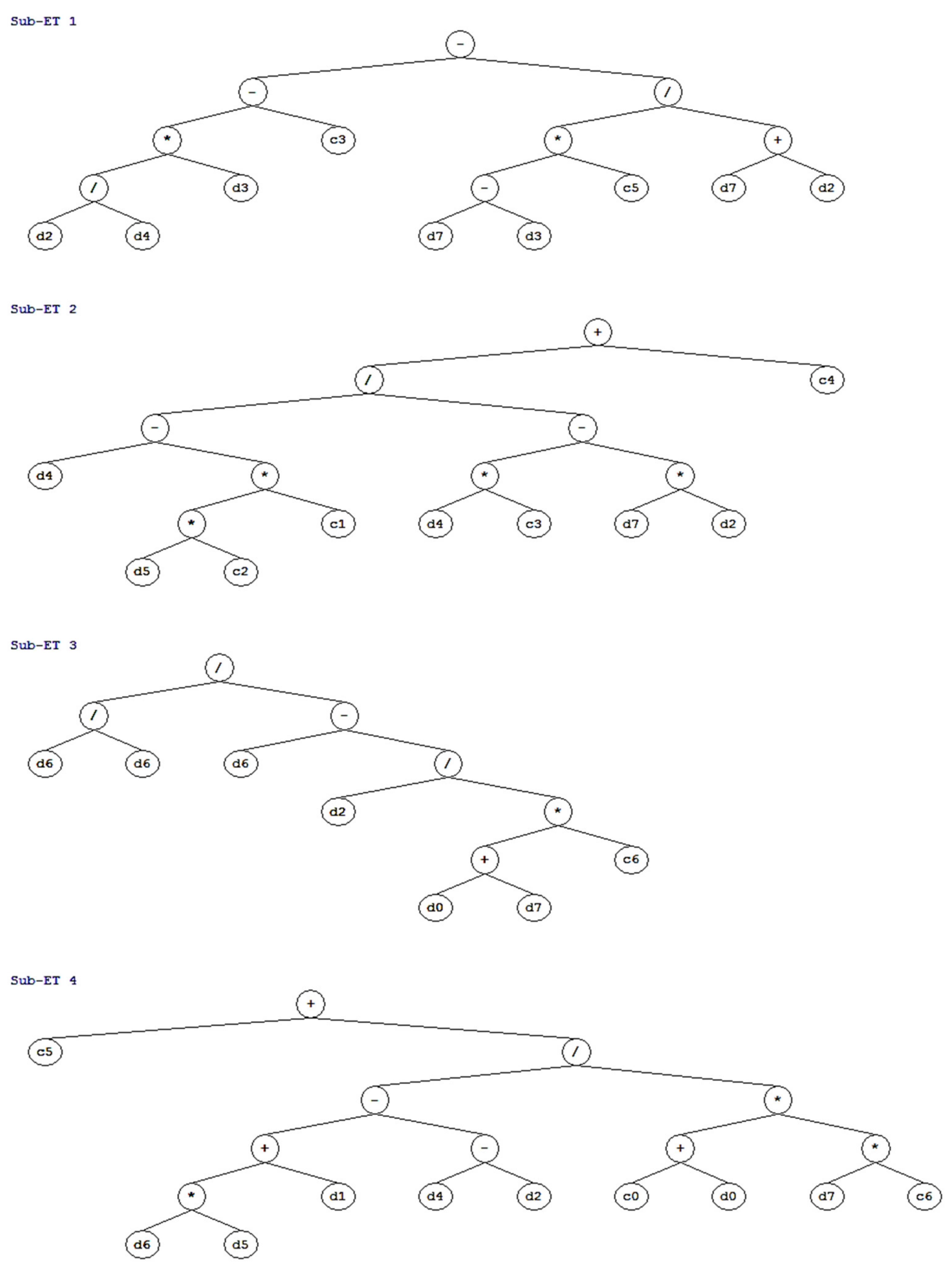
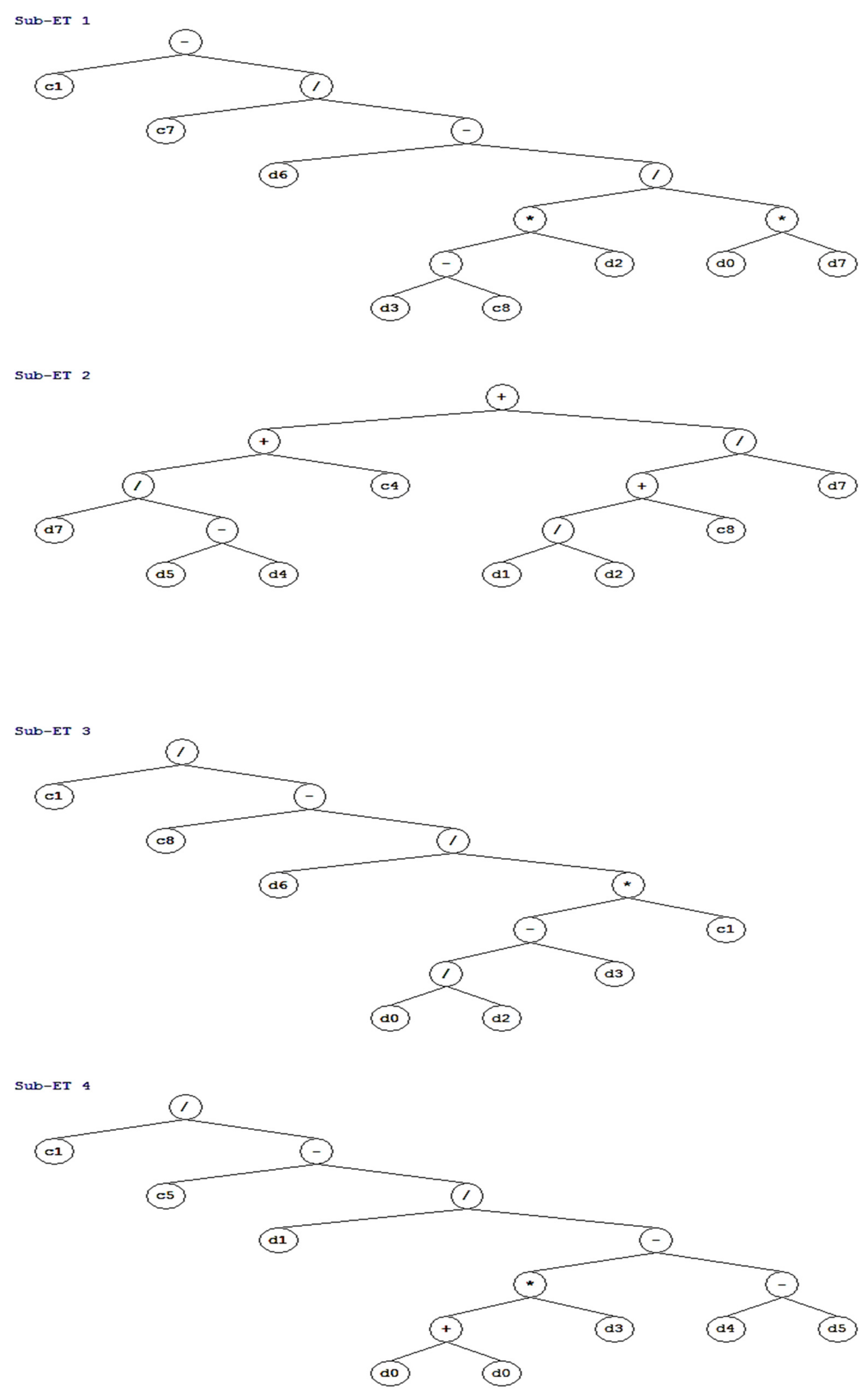
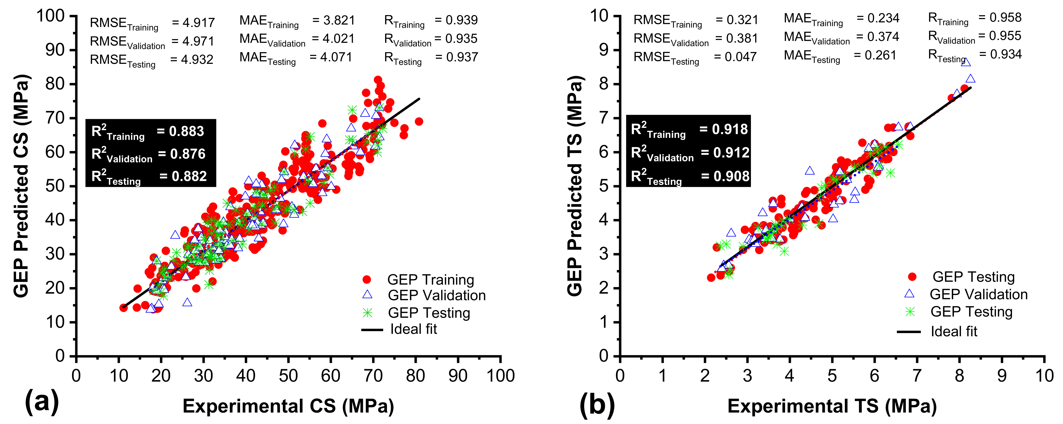
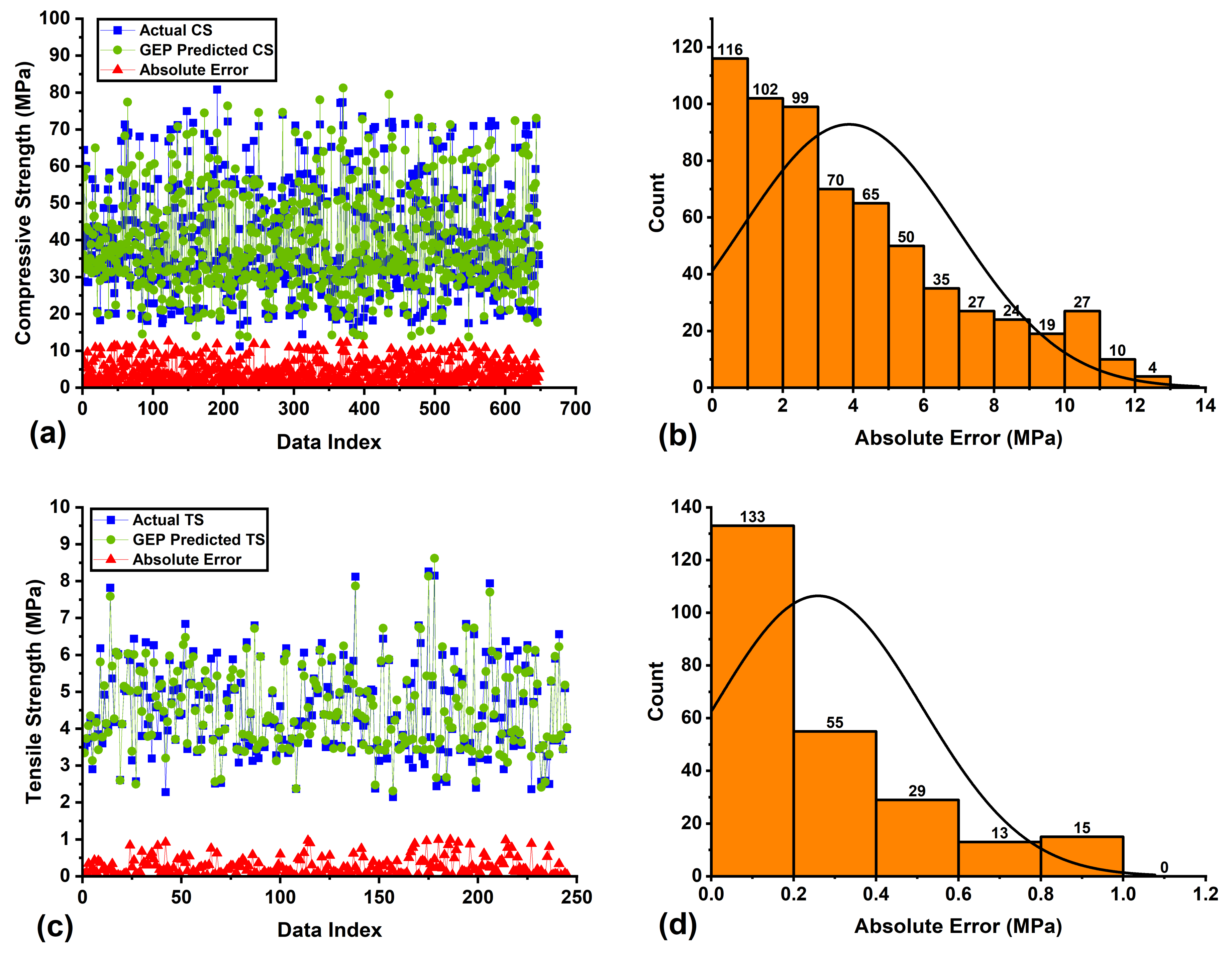
3.3. GEP Model Development and Performance Assessment

Unlike the other models, GEP also provides predictive equations for the outputs. So, before discussing the performance of GEP models, the development of predictive equations for the CS and TS of concrete is described in detail. The efficacy of the GEP-based developed models is significantly influenced by their fitting parameters. Therefore, it is crucial to find the best parametric settings to achieve an appropriate balance between complexity and simplicity, avoid overfitting, and enhance the model’s generalization capability. The process of identifying the most suitable parameter values for a model that exhibits strong performance on new data generally involves an iterative procedure. In the present study, a trial-and-error approach was employed. During the experimentation phase of GEP, various combinations of parameters were tested by varying the genetic factor (chromosomes), the linking function, the head size, and the number of genes to identify the best parametric settings for both the CS and TS models, as presented in Table 8 and Table 9, respectively. The GEP system was designed to run indefinitely due to the significance of maintaining stable values for correlations and fitness functions. The models were evaluated based on several statistical error measures, such as R², RMSE, and MAE values. The statistical measures for the training and evaluation phases of the GEP models for CS are displayed in

Table 12. Summary of the GEP models for CS.

Models	Training Dataset						Testing (Validation) Dataset
	R2	RMSE	MAE	RRSE	R	ρ	R2	RMSE	MAE	RRSE	R	ρ
CS1	0.861	5.047	4.070	0.374	0.928	0.107	0.839	5.277	4.071	0.402	0.916	0.110
CS2	0.860	5.079	4.069	0.375	0.927	0.108	0.852	5.031	4.098	0.387	0.923	0.111
CS3	0.863	4.960	4.069	0.370	0.929	0.107	0.857	4.997	4.065	0.379	0.926	0.110
CS4	0.871	4.934	4.063	0.357	0.933	0.102	0.861	4.957	4.060	0.366	0.928	0.106
CS5	0.870	4.959	4.061	0.362	0.933	0.104	0.881	4.967	4.087	0.345	0.939	0.108
CS6	0.767	7.691	5.085	0.483	0.876	0.166	0.784	6.738	5.030	0.465	0.885	0.169
CS7	0.798	6.871	5.075	0.463	0.893	0.177	0.805	6.401	5.074	0.457	0.897	0.180
CS8	0.798	6.871	5.075	0.463	0.893	0.123	0.805	6.401	5.064	0.468	0.897	0.127
CS9	0.857	5.046	4.066	0.346	0.926	0.095	0.857	5.035	4.071	0.385	0.925	0.099
CS10	0.866	5.002	4.068	0.366	0.930	0.094	0.869	4.988	4.063	0.366	0.932	0.098
CS11	0.876	4.998	3.98	0.376	0.936	0.085	0.875	4.935	4.062	0.366	0.936	0.088
CS12	0.883	4.917	3.821	0.341	0.940	0.064	0.876	4.972	4.021	0.356	0.936	0.067
CS13	0.882	4.922	3.881	0.344	0.939	0.069	0.872	4.985	4.065	0.359	0.934	0.072
CS14	0.881	4.949	3.897	0.345	0.939	0.069	0.881	4.997	4.058	0.346	0.938	0.072
CS15	0.860	5.759	4.071	0.462	0.927	0.099	0.861	4.967	4.071	0.400	0.928	0.102
CS16	0.778	6.691	5.082	0.483	0.882	0.156	0.787	6.634	5.083	0.467	0.887	0.159
CS17	0.808	5.875	4.945	0.463	0.899	0.167	0.805	6.401	4.865	0.447	0.897	0.170
CS18	0.818	5.781	4.936	0.433	0.905	0.125	0.805	6.401	4.826	0.436	0.897	0.128
CS19	0.860	5.079	4.069	0.375	0.927	0.103	0.852	4.931	4.869	0.387	0.923	0.107
CS20	0.861	5.035	4.068	0.373	0.928	0.102	0.846	5.073	4.888	0.393	0.920	0.106

, while these measures for the TS models are shown in

Table 13. Summary of the GEP models for TS.

Models	Training Dataset						Testing (Validation) Dataset
	R2	RMSE	MAE	RRSE	R	ρ	R2	RMSE	MAE	RRSE	R	ρ
TS1	0.896	0.365	0.265	0.312	0.947	0.058	0.871	9.277	0.385	0.353	0.933	0.059
TS2	0.895	0.379	0.275	0.313	0.946	0.058	0.884	8.931	0.395	0.340	0.940	0.060
TS3	0.899	0.396	0.245	0.309	0.948	0.058	0.889	8.747	0.395	0.333	0.943	0.059
TS4	0.907	0.353	0.242	0.298	0.952	0.055	0.892	7.597	0.392	0.322	0.945	0.057
TS5	0.906	0.376	0.242	0.302	0.952	0.056	0.913	7.967	0.382	0.303	0.956	0.058
TS6	0.803	0.469	0.367	0.403	0.896	0.089	0.816	10.738	0.387	0.409	0.903	0.091
TS7	0.834	0.427	0.341	0.387	0.913	0.095	0.836	10.401	0.381	0.401	0.914	0.097
TS8	0.834	0.411	0.342	0.387	0.913	0.067	0.836	10.401	0.384	0.411	0.914	0.068
TS9	0.892	0.388	0.276	0.289	0.945	0.052	0.888	8.346	0.387	0.339	0.942	0.053
TS10	0.902	0.367	0.245	0.306	0.949	0.051	0.901	8.430	0.382	0.321	0.949	0.053
TS11	0.912	0.345	0.239	0.315	0.955	0.046	0.907	8.257	0.379	0.284	0.952	0.047
TS12	0.919	0.321	0.234	0.285	0.959	0.035	0.908	7.972	0.374	0.312	0.953	0.036
TS13	0.918	0.322	0.238	0.287	0.958	0.037	0.904	8.283	0.378	0.315	0.951	0.039
TS14	0.917	0.349	0.237	0.288	0.958	0.037	0.912	7.997	0.377	0.304	0.955	0.039
TS15	0.896	0.359	0.255	0.386	0.946	0.054	0.893	8.967	0.385	0.351	0.945	0.055
TS16	0.814	0.491	0.366	0.403	0.902	0.084	0.818	10.634	0.386	0.410	0.905	0.086
TS17	0.844	0.487	0.356	0.387	0.919	0.090	0.836	10.401	0.396	0.392	0.914	0.092
TS18	0.854	0.478	0.345	0.362	0.924	0.067	0.836	10.401	0.391	0.383	0.914	0.069
TS19	0.895	0.379	0.245	0.313	0.946	0.056	0.884	8.931	0.385	0.340	0.940	0.058
TS20	0.897	0.387	0.247	0.312	0.947	0.055	0.878	9.073	0.387	0.345	0.937	0.057

. The results demonstrate that increasing the parametric values (head size, genetic factors, linking functions, and gene size) while using different linking functions (+, −, /, ×) enhanced model performance, as reflected by lower RMSE and MAE values and higher R² values. Moreover, the running time and the complication of the models may be increased by the increase in these parametric values, thereby making it difficult to comprehend the dynamics of the model. Following the statistical assessments conducted on the suggested GEP models, the best GEP models (CS12 and TS12) were chosen to predict the CS and TS of concrete incorporated with SF and GGBS, respectively.

The output of the optimum GEP models used for predicting CS and TS are shown in the form of expression trees (ETs), as displayed in Figure 14 and Figure 15. The ETs for CS and TS include four fundamental mathematical operations, namely +, /, −, and x, as illustrated in Table 8. These ETs were interpreted to establish the empirical correlations. The empirical expressions for the CS models are developed by considering multiplication as a linking function. The head size and the number of genes are considered as 10 and 4, respectively. The simplified equations in Equations (22)–(26) are recommended for predicting the CS of concrete containing SF and GGBS. The indicators used in the ETs are presented in

Table 14. ET indicators.

Parameter	Unit	Indicator in the Expression Tree	Description
C	kg/m3	d0	Cement content
GGBS	kg/m3	d1	Amount of GGBS
SF	kg/m3	d2	Amount of silica fume
SP	kg/m3	d3	Superplasticizer
CA	kg/m3	d4	Coarse aggregates (granite)
FA	kg/m3	d5	Fine aggregates
W/B	-	d6	Water-to-cement ratio
Age	Days	d7	Age of specimens at the time of testing

.

$$\mathrm{CS} \left(\mathrm{MPa}\right)=\mathrm{A}\times \mathrm{B}\times \mathrm{C}\times \mathrm{D}$$

(22)

$$\mathrm{A}=\frac{2.15\left(\mathrm{d}7-\mathrm{d}3\right)}{\mathrm{d}7+\mathrm{d}2}+\frac{\mathrm{d}2}{\mathrm{d}4}\mathrm{d}3+2.62$$

(23)

$$\mathrm{B}=\left[\mathrm{d}4-\frac{14·\mathrm{d}5}{-4.38·\mathrm{d}4-\mathrm{d}7·\mathrm{d}2}\right]+9.03$$

(24)

$$\mathrm{C}=\frac{4·\mathrm{d}6\left(\mathrm{d}0+\mathrm{d}7\right)}{4·\mathrm{d}6\left(\mathrm{d}0+\mathrm{d}7\right)-\mathrm{d}2}$$

(25)

$$\mathrm{D}=0.3939+\frac{\left(\mathrm{d}5·\mathrm{d}6+\mathrm{d}1\right)-\left(\mathrm{d}4-\mathrm{d}2\right)}{\mathrm{d}7\left(5.31·\mathrm{d}0-69.56\right)}$$

(26)

The formula for the TS of concrete incorporated with SF and GGBS is created by considering the same parameters as those considered for the CS. Parametric settings for the optimum proposed model (TS12) are illustrated in Table 9. The empirical Equations (27)–(31) are proposed to predict TS.

$$\mathrm{TS}=\mathrm{E}\times \mathrm{F}\times \mathrm{G}\times \mathrm{H}$$

(27)

$$\mathrm{E}=-1.5-\frac{1.11.\mathrm{d}0·\mathrm{d}7}{\mathrm{d}6·\mathrm{d}0·\mathrm{d}7-\mathrm{d}2·\left(\mathrm{d}3-4.67\right)}$$

(28)

$$\mathrm{F}=\frac{\mathrm{d}7}{\mathrm{d}5-\mathrm{d}4}+\frac{\mathrm{d}1+9.66·\mathrm{d}2}{\mathrm{d}7·\mathrm{d}2}-8.32$$

(29)

$$\mathrm{G}=\frac{-2.47}{-7.2-\frac{\mathrm{d}6}{\left(\frac{\mathrm{d}0}{\mathrm{d}2}-\mathrm{d}3\right)\left(-7.2\right)}}$$

(30)

$$\mathrm{H}=\frac{-4.98·\mathrm{d}0·\mathrm{d}3+2.49\left(\mathrm{d}4-\mathrm{d}5\right)}{-14.32·\mathrm{d}0.\mathrm{d}3+7.16\left(\mathrm{d}4-\mathrm{d}5\right)-\mathrm{d}1}$$

(31)

In addition, statistical analyses of the GEP-based model outcomes are shown in Figure 16a,b. It can be noticed that the MAE and RMSE values obtained from the CS-GEP and TS-GEP models are comparatively greater than those obtained from the ANN and ANFIS models. The CS-GEP models show 22% and 47% higher values of RMSE in the testing phase compared to the ANN and ANFIS values, respectively. For TS-GEP, these values are 15% and 20% higher, respectively. Similarly, the R² values for the evaluation phase are 0.88 and 0.90, respectively, for the CS-GEP and TS-GEP models, which are 7% and 3% lower than the ANN models, whereas these values are 9% and 10% lower than the ANFIS models. Other statistical error values, including the RSE and RRMSE calculated for the GEP models, are comparable to ANN and ANFIS-based models for CS and TS. The results of the error analysis of the GEP-based predictive models for CS and TS are shown in Figure 17a–d. It can be noted that the absolute error values between the GEP-anticipated and actual values are slightly higher for CS and lower for TS, in contrast to those of the ANN and ANFIS models. Moreover, as shown in Figure 17b,d, 60% of the error values of CS-GEP fall in the range of 0–4 MPa. Similarly, 77% of the error values of TS-GEP fall in the range of 0–0.4 MPa, which is relatively less than the ANN and ANFIS models. The possible reason for the discrepancy in the relative efficacy of the ANN, ANFIS, and GEP models for CS and TS could be attributed to the variability in the corresponding experimental datasets. The GEP-based empirical algorithm has demonstrated superior predictive performance compared to the ANN and ANFIS when applied to larger datasets.

The GEP-based developed models for CS and TS were further evaluated by using the correlation p-values, which represent the likelihood of significance. The statistical analysis was conducted using the SPSS v23 software, which is commonly employed in practical applications. A significance threshold of 5% was used in the computation, as reported by Güllü and Fedakar [93]. The p-value indicates the degree of confirmation against the null hypothesis, in which a lower p-value corresponds to a greater degree of confirmation. The p-values obtained for the GEP models for CS and TS are close to zero, indicating a significant degree of correlation between the observed and projected values.

3.4. Experimental Validation

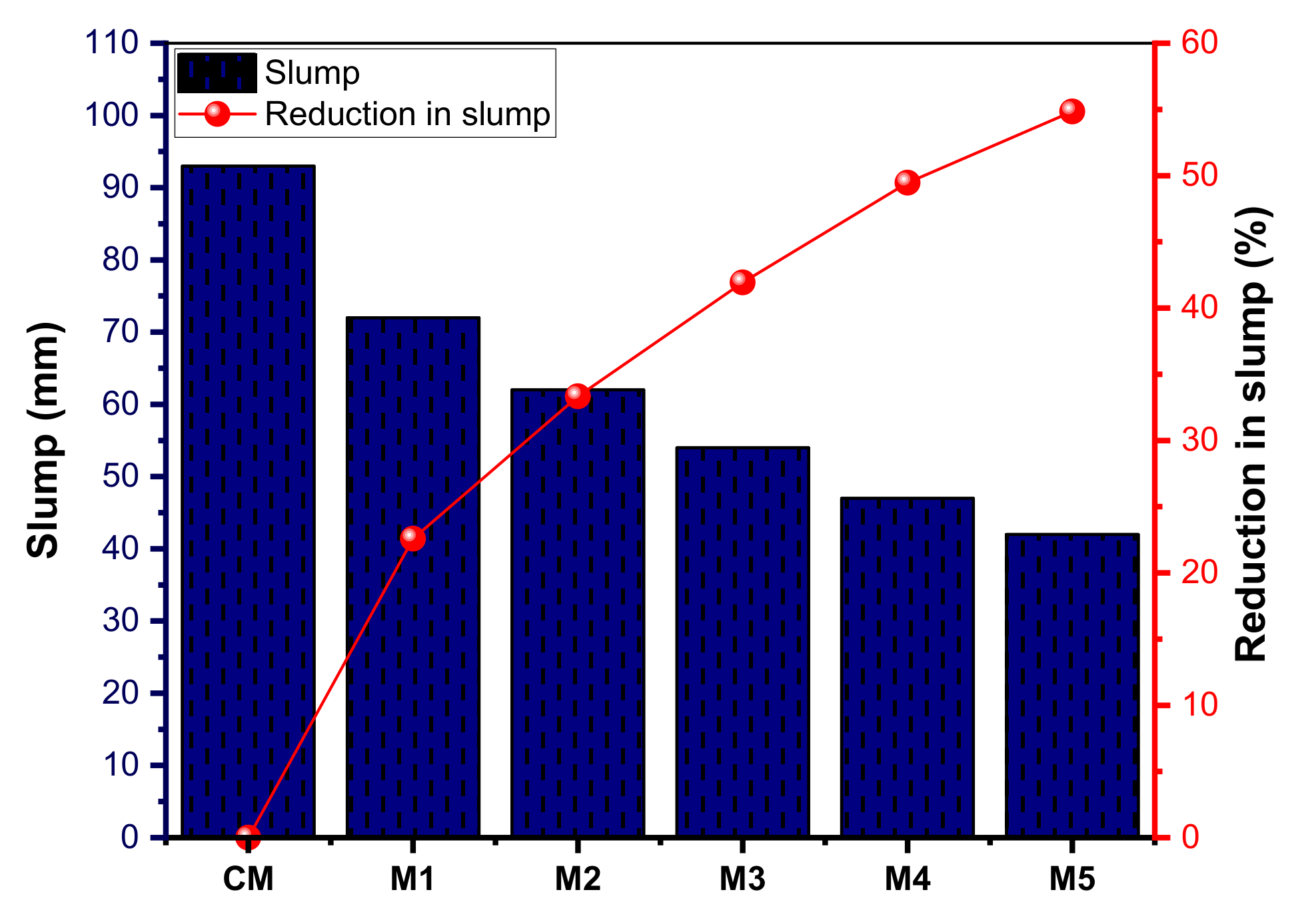
3.4.1. Workability

Figure 18 displays the slump readings for all six tested combinations. The minimum slump reading of 42 mm was noted in a mixture containing 20% SF and 40% GGBS, which is 55% less than the control mix. It is clear that slump readings decrease with an increase in the cement replacement level with SCMs (SF and GGBS) in the concrete. This is due to the fact that SF and GGBS have greater specific surface area and more cohesion, which requires extra water to maintain workability compared to normal concrete [54].

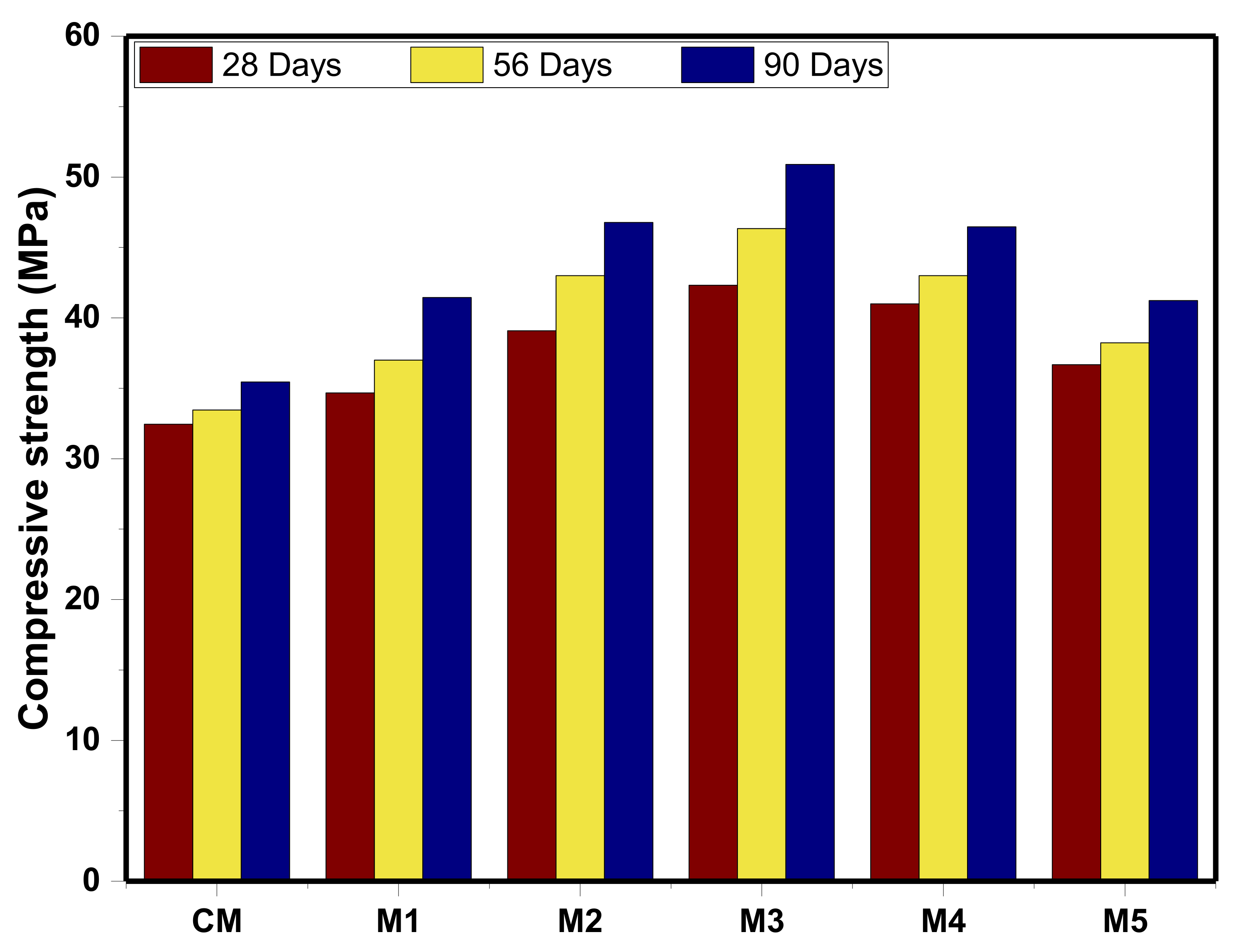
3.4.2. Compressive Strength

The CS was determined using the compression testing machine, following the guidelines of the ASTM C39. The results of the laboratory-derived CS are shown in Figure 19. It can be noted that CS increased with the increase in the age of testing, irrespective of the specific binder mixture employed for the development of the samples. The increment in CS at later ages with the addition of SF and GGBS is more pronounced than in CM. This is because of the pozzolanic reactions and nucleation effects associated with SF that reduce the calcium hydrate (CH) content and enhance the densification of the samples. Further, the enhanced CS at later ages can also be attributed to the fine grain sizes and filler effects due to the inclusion of SF and GGBS [94]. The concrete mix containing SCMs (10% SF and 30% GGBS) demonstrated the highest CS of 50.4 MPa at the age of 90 days. The optimum replacement of SCMs resulted in 21% enhanced CS as compared to CM. Meanwhile, the addition of SCMs exceeding 40% (M5 mix) led to a decrease in CS by 11%. This is due to the fact that excessive substitution of cement with supplementary cementitious materials (SCMs) could reduce the presence of reactive substances needed for hydration, resulting in weaker connections and weakened durability in the hardened concrete [54]. It is important to mention that ACI-recommended conversion factors were used to convert the CS values into TS values [95].

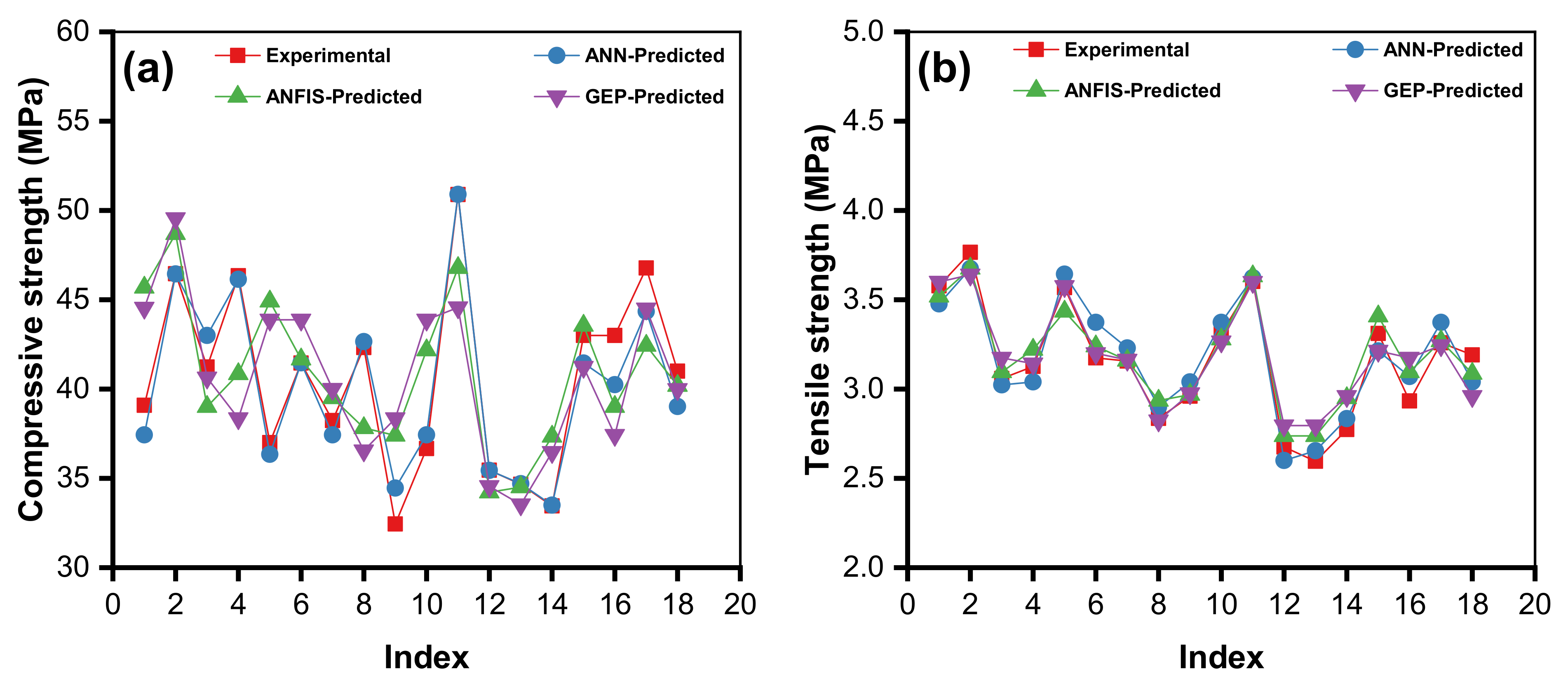
3.4.3. Comparison of Experimental Results with Proposed Models

After thorough evaluations of the models using various mathematical approaches, a separate dataset was constructed using experimental testing to evaluate the effectiveness and applicability of the produced ML models. The separate dataset allows a thorough evaluation of the model’s ability to make predictions without relying on the initial data used for training. A statistical summary of the constructed dataset using experimental findings is presented in

Table 15. Statistical summary of the developed database for external validation.

Parameters	Cement	Water	SF	GGBS	CA	FA	Age	CS	TS
	(kg/m3)	(kg/m3)	(kg/m3)	(kg/m3)	(kg/m3)	(kg/m3)	(Days)	(MPa)	(MPa)
Mean	283.67	156	41.17	90	1050	730	59.56	40.53	3.16
Median	270	156	104	1050	730	56	41.12	3.17
SD	84.28	0	57.56	0	0	25	5.1	0.33
Range	249	0	166	0	0	62	18.45	1.17
Minimum	166	156	0	1050	730	28	32.44	2.6
Maximum	415	156	166	1050	730	90	50.89	3.77

. This cross-validation approach is crucial for confirming the models’ ability to generalize to unfamiliar data, which is a vital part of their practical applications. It is important to mention that the same parametric settings were used in the development of the models so that hyperparameter optimization can also be verified.

A comparison between the findings of the external experimental validation and ML models is depicted in Figure 20a,b for the CS and TS models, respectively. It can be seen that the findings are highly comparable, with an R² of more than 0.88 in all developed models, as shown in Figure 21a,b for CS and TS, respectively. Furthermore, the error percentage between the experimental and estimated values falls in the acceptable range of less than 10%, as shown in

Table 16. Percentage error comparison between the model-predicted and experimental values.

CS Experimental Values	Error % in ML Models			TS Experimental Values	Error % in ML Models
	ANN	ANFIS	GEP		ANN	ANFIS	GEP
39.09	4.24	1.67	4.12	3.58	2.82	1.64	0.63
46.46	0.03	4.33	2.61	3.77	2.41	2.40	3.34
41.23	4.29	2.03	6.30	3.06	1.16	1.21	3.80
46.34	0.42	4.50	1.88	3.13	2.78	3.02	0.48
37.00	1.78	3.08	5.31	3.57	2.10	3.75	0.22
41.45	0.04	1.06	6.42	3.17	6.25	2.06	0.79
38.23	2.09	3.66	2.44	3.16	2.31	0.10	0.20
42.32	0.78	6.70	3.13	2.84	2.26	3.50	0.44
32.44	6.20	1.08	3.66	2.96	2.71	0.29	0.54
36.67	2.07	1.91	2.04	3.31	1.88	0.96	1.39
50.89	0.03	0.03	4.73	3.60	0.60	0.83	0.09
35.45	0.02	2.32	3.32	2.68	2.84	2.32	4.48
34.67	0.11	6.38	3.38	2.60	2.27	5.51	7.74
33.45	0.15	7.71	5.19	2.77	2.19	6.37	6.73
43.00	3.60	1.28	4.11	3.31	2.96	2.93	2.95
43.00	6.42	6.37	2.05	2.93	4.65	5.51	8.22
46.78	5.20	0.26	5.15	3.26	3.52	0.30	0.42
41.00	4.82	3.04	3.53	3.19	4.74	3.30	7.26

. Minor differences can be noted between the outcomes of the actual and validation models, which can be due to the lower number of databases used for validation. The optimum replacement in the experimental validation is found to be 10% SF and 30% GGBS, which is well aligned with the literature. The consistency of the results demonstrates the efficacy of the models in accurately identifying and anticipating the fundamental patterns of mechanical characteristics of concrete incorporated with SF and GGBS. The strong alignment between the model predictions and the findings obtained in the laboratory highlights the reliability of the ML models that have been constructed, thus evoking confidence in their dependability for real-world use.

3.5. Statistical Evaluation and Comparative Analysis of Models

The comparative analysis based on statistical parameters of the proposed models employing the ANNs, ANFIS, and GEP is presented in

Table 17. Summary of statistical calculations.

Proposed Models		Subset Type	R2	RMSE	MAE	RRMSE	RSE	R	ρ	OF
CS	ANN	Trn-set	0.9419	3.3284	1.788	0.0851	0.0583	0.9705	0.0436	0.0427
		Vald-set	0.9377	4.0493	2.791	0.1008	0.0647	0.9683	0.0512
		Test-set	0.938	3.8269	2.832	0.0925	0.0657	0.9685	0.0472
	ANFIS	Trn-set	0.9702	2.3688	1.681	0.0731	0.0298	0.985	0.031	0.0311
		Vald-set	0.9698	3.0691	2.321	0.0859	0.0583	0.9848	0.0436
		Test-set	0.9678	2.5721	1.983	0.0659	0.0339	0.9838	0.03325
	GEP	Trn-set	0.8831	4.9174	3.821	0.1251	0.1161	0.9392	0.0642	0.0621
		Vald-set	0.8763	4.9716	4.021	0.1263	0.1243	0.9353	0.0841
		Test-set	0.8821	4.9321	4.071	0.1255	0.1191	0.9371	0.0737
TS	ANN	Trn-set	0.9585	0.2699	0.202	0.0592	0.2675	0.979	0.0299	0.0299
		Vald-set	0.9384	0.3211	0.255	0.0723	0.0671	0.9681	0.0366
		Test-set	0.9311	0.3433	0.258	0.0761	0.0692	0.9654	0.0392
	ANFIS	Trn-set	0.9951	0.0886	0.034	0.0198	0.0167	0.9975	0.0099	0.0099
		Vald-set	0.9981	0.0381	0.133	0.0077	0.0021	0.9991	0.0039
		Test-set	0.998	0.0383	0.017	0.0076	0.002	0.9992	0.0038
	GEP	Trn-set	0.9188	0.3213	0.234	0.0712	0.0812	0.9585	0.0362	0.035
		Vald-set	0.9123	0.3812	0.374	0.0782	0.0891	0.9551	0.0426
		Test-set	0.9081	0.4043	0.261	0.0861	0.0972	0.9342	0.0533

Note: Trn: training, Vald: validation, Test: testing.

. The proposed models efficiently predicted the CS and TS of concrete containing SCMs by considering the impact of all specified input parameters, as is obvious from the significantly reduced errors (RMSE, MAE, and RSE). The R² values for the CS neural models using ANN and ANFIS methods are around 95% and 99%, respectively, for all three datasets (training, validation, and testing), while they are just below 90% for the GEP models. Likewise, the other statistical errors, such as RMSE and MAE for the CS models, are lowest for the ANFIS, followed by the ANNs. The mean R value for all three proposed models is higher than 90%. The higher R values indicate a strong connection between the input parameters, which results in higher prediction accuracy [80]. Similarly, the ANFIS models exhibit higher R² values in all three datasets for TS. All of the proposed models for TS showed R² values greater than 90% in the following order: R²_ANFIS 0.99 > R²_ANN 0.95 > R²_GEP 0.91. The superior results indicated by the ANFIS models can be attributed to the integration of the neural networks’ training capability and the fuzzy logic’s reasoning ability. The predictive capabilities of the established models are also compared based on statistical performance measures such as PI and OF, as depicted in Figure 22a–d. The values of these measures being nearer to zero indicate the better precision of the models. In the established models for CS, the ANFIS models show the lowest PI, equal to 0.031, 0.043, and 0.033 in the training, validation, and testing phases, respectively; for CS-ANN, these values are 0.043, 0.051, and 0.047, respectively. Similarly, the PI values in the case of CS using GEP are 0.064, 0.084, and 0.073 for the training, testing, and validation phases, respectively. Additionally, for the TS models, the PI is lower than 1% for all three testing conditions. According to the criteria discussed by [85], the PI value should be less than 20% for accurate prediction. Hence, all of the developed models satisfy the given criteria and can be considered good for the anticipation of the CS and TS of concrete incorporated with SF and GGBS. However, in the ANN models, significant variation was observed between PI values of the training and testing conditions. As discussed in a recent study by Jalal et al. [85], this variation can be attributed to the local minima problem that is commonly associated with ANN models. According to Zhang et al. [88], the optimizing process may cease at a locally optimized state rather than a global termination state, leading to inaccurate predictions. The concept of local optimization involves the closure of the search process for a particular problem when the ideal solution is discovered, even before the optimum one. However, in ANFIS models, the aforementioned issue can be addressed by the training capacity of the ANN and the fuzzification of logical reasoning in the fuzzy toolbox. Furthermore, it can be noted that the OF values obtained from the ANN, ANFIS, and GEP models for CS are 0.042, 0.031, and 0.062, respectively, and for the TS models, these values are 0.029, 0.009, and 0.035, respectively. The OF values for all cases are close to zero, revealing the validity of the proposed models while controlling the overfitting.

The summary of statistical measures indicates that in all predictive models, namely the ANN, ANFIS, and GEP models, the projected values are very close to actual values for both the CS and TS. Considering the R and R² values, the upward sequence is ANFIS > ANN > GEP. Meanwhile, the ANFIS models for both CS and TS exhibit the lowest values for error measures (RMSE, RSE, MAE, RRMSE) followed by the ANN and GEP models. However, the GEP models show superior performance compared to the ANFIS and ANN models with respect to the closeness of the RMSE, MAE, RSE, and R² values between the training, validation, and testing sets for both CS and TS. In addition, GEP represents an evolutionary technique that gives a simple empirical formula for forecasting the CS and TS (refer to Equations (25) and (26)). This approach significantly diminishes the overall duration needed to estimate the CS and TS compared with conventional testing procedures (i.e., experimental investigations), and the evaluation process can be completed at a significantly faster rate. Therefore, the application of the presented equations gives a viable and quick method for the estimation of the CS and TS of concrete incorporated with SF and GGBS.

3.6. Validation of GEP-Based Equations

The best-proposed model (GEP) was further validated by using several statistical tests, as shown in

Table 18. GEP model external validation.

S. No.	Equation	Condition	Model
			CS	TS
1	$\mathrm{R}$	$\mathrm{R}>0.8$	0.991	0.993
2	$\mathrm{k}={{\displaystyle \sum }}_{\mathrm{i}=1}^{\mathrm{n}}\frac{({\mathrm{a}}_{\mathrm{i}}\times {\mathrm{m}}_{\mathrm{i}})}{{{\mathrm{a}}_{\mathrm{i}}}^2}$	$0.85<\mathrm{k}<1.15$	0.971	0.973
3	${\mathrm{k}}^{\prime }={{\displaystyle \sum }}_{\mathrm{i}=1}^{\mathrm{n}}\frac{({\mathrm{a}}_{\mathrm{i}}\times {\mathrm{m}}_{\mathrm{i}})}{{{\mathrm{m}}_{\mathrm{i}}}^2}$	$0.85<{\mathrm{k}}^{\prime }<1.15$	1.002	1.001
4	${{\mathrm{R}}_0}^2=1-\frac{{{\displaystyle \sum }}_{\mathrm{i}=1}^{\mathrm{n}}{\left({\mathrm{m}}_{\mathrm{i}}-{{\mathrm{a}}_{\mathrm{i}}}^0\right)}^2}{{{\displaystyle \sum }}_{\mathrm{i}=1}^{\mathrm{n}}{\left({\mathrm{m}}_{\mathrm{i}}-{{\mathrm{m}}_{\mathrm{i}}}^0\right)}^2}$, ${{\mathrm{a}}_{\mathrm{i}}}^0=\mathrm{k}\times {\mathrm{m}}_{\mathrm{i}}$	${{\mathrm{R}}_0}^2\cong 1$	0.969	0.970
5	${{{\mathrm{R}}^{\prime }}_0}^2=1-\frac{{{\displaystyle \sum }}_{\mathrm{i}=1}^{\mathrm{n}}{\left({\mathrm{a}}_{\mathrm{i}}-{{\mathrm{m}}_{\mathrm{i}}}^0\right)}^2}{{{\displaystyle \sum }}_{\mathrm{i}=1}^{\mathrm{n}}{\left({\mathrm{a}}_{\mathrm{i}}-{{\mathrm{a}}_{\mathrm{i}}}^0\right)}^2}$, ${{\mathrm{m}}_{\mathrm{i}}}^0={\mathrm{k}}^{\prime }\times {\mathrm{a}}_{\mathrm{i}}$	${{{\mathrm{R}}^{\prime }}_0}^2\cong 1$	0.990	0.991
6	$\mathrm{m}=\frac{\left({\mathrm{R}}^2-{{\mathrm{R}}_0}^2\right)}{{\mathrm{R}}^2}$	$\mathrm{m}<1$	0.0541	0.055
7	$\mathrm{n}=\frac{\left({\mathrm{R}}^2-{{{\mathrm{R}}^{\prime }}_0}^2\right)}{{\mathrm{R}}^2}$	$\mathrm{n}<1$	0.005	0.005

. Golbraikh et al. [96] recommended that to achieve higher efficiency in the model, the gradient of one of the regression lines (k or k′) crossing through the origin (center) must pass close to unity. The gradient of the regression lines for the CS model is 0.971, while for TS, it is 0.973. In addition, performance indicators (i.e., m and n) of less than 0.1 are considered reliable. This signifies a strong correlation and more accuracy. It can be seen that both CS and TS models exhibit m and n values less than the recommended range. Moreover, several researchers have recommended that the squared coefficient (R₀²) between actual and estimated values should also be close to 1 [97]. It is evident from the findings that the suggested models satisfy the external verification requirements, demonstrating the models’ excellent validity, prediction power, and independence from simple correlations between the inputs and outputs.

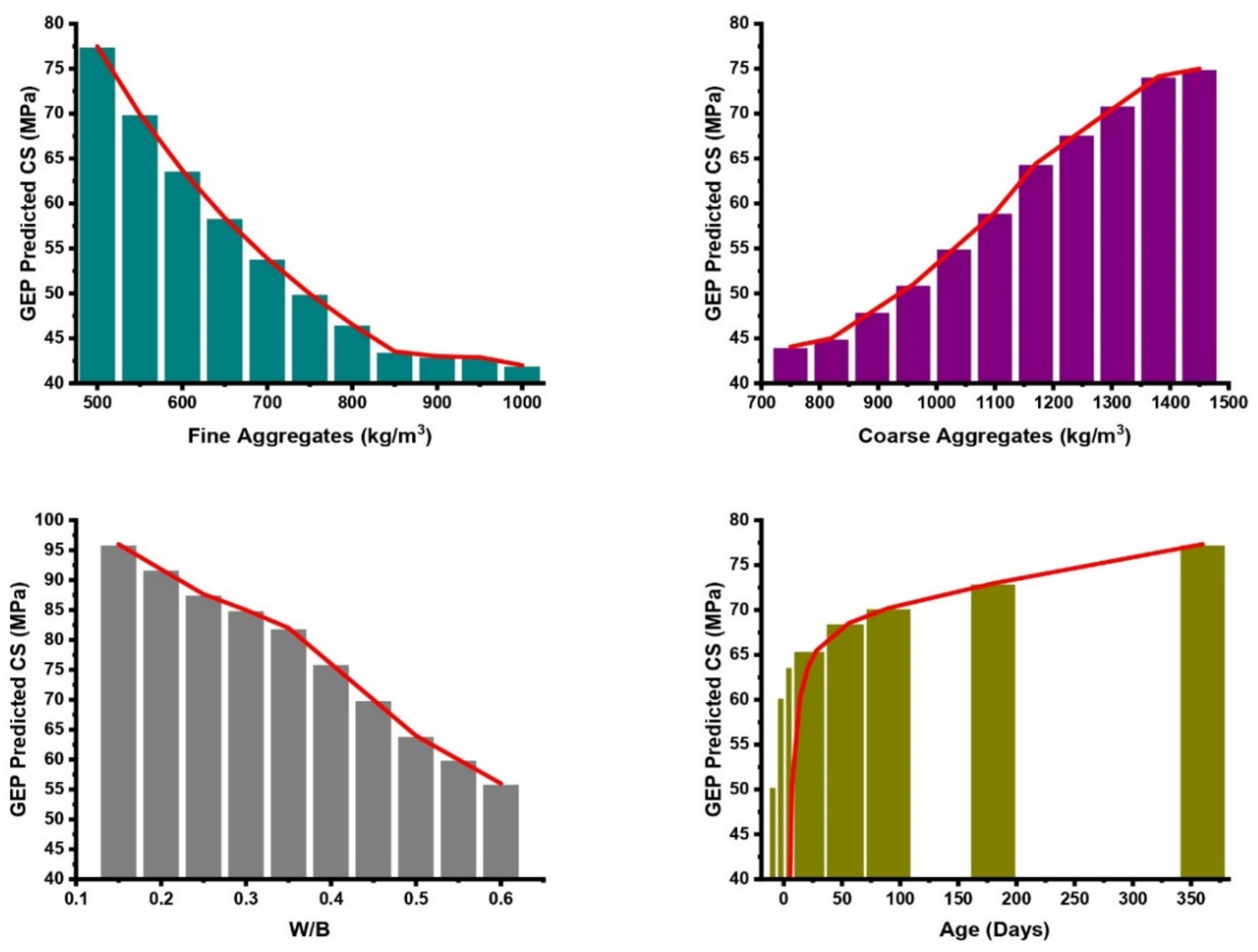
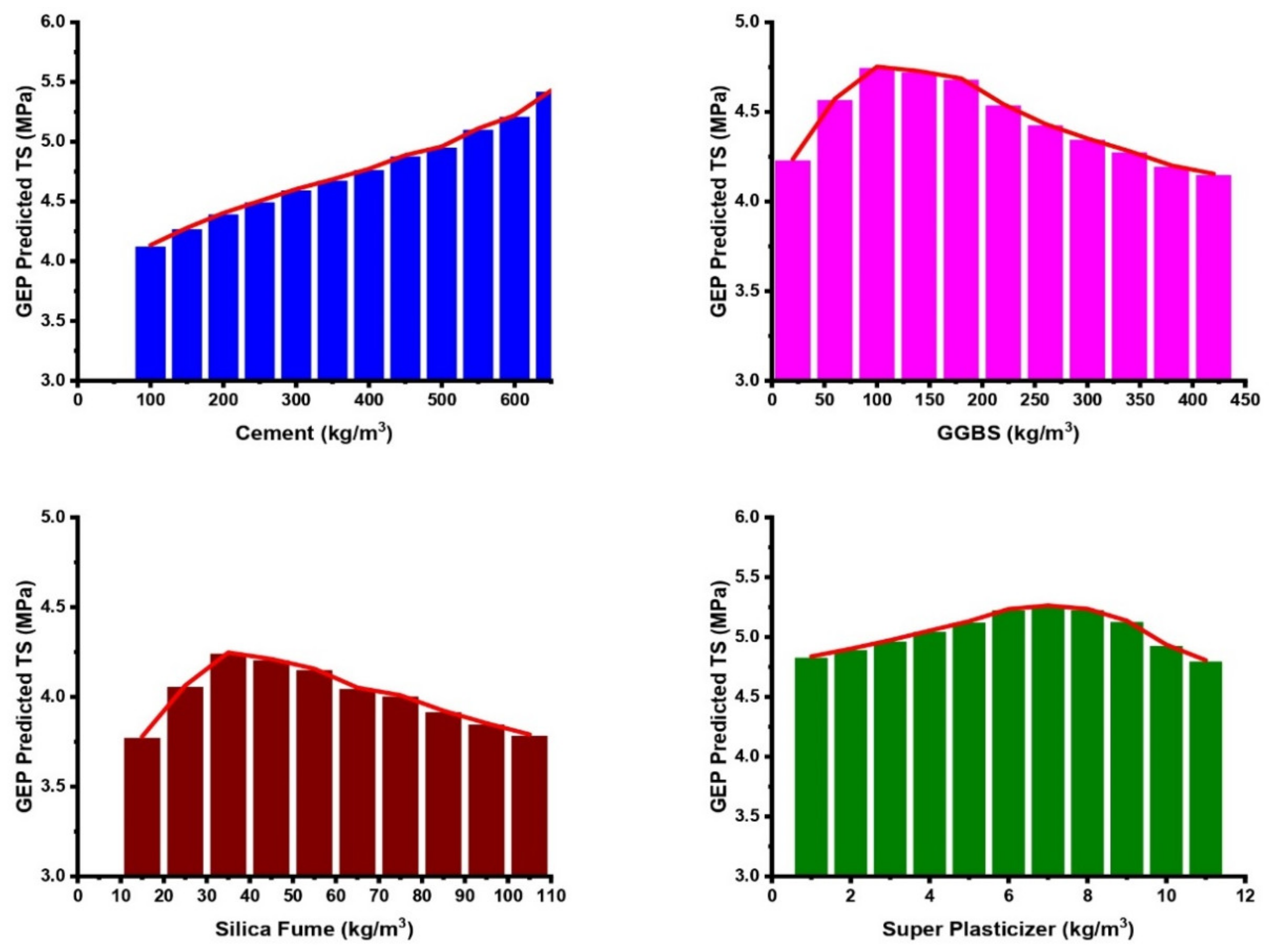
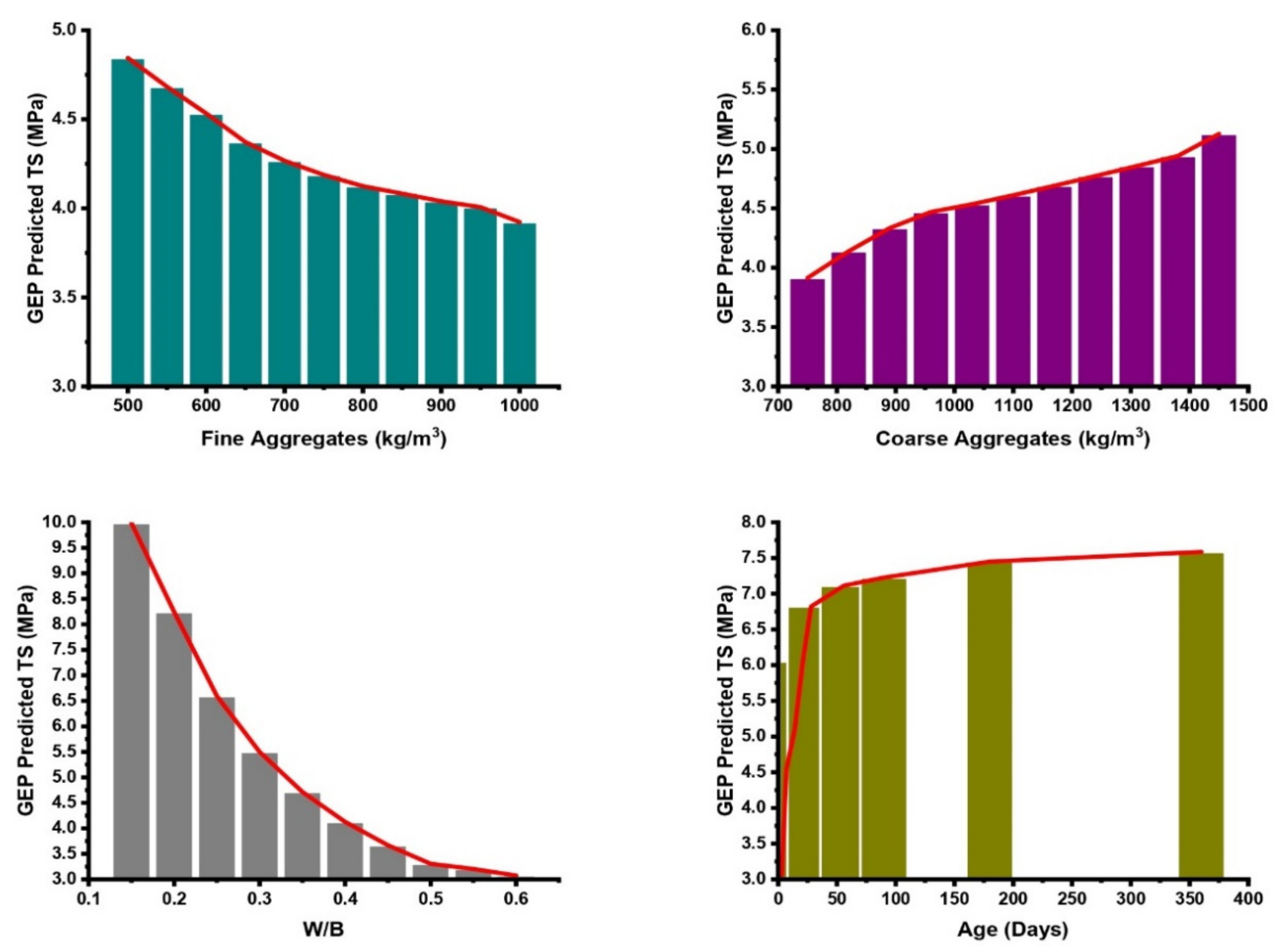
3.7. Sensitivity and Parametric Analyses

In the case of modeling based on machine learning, multiple parametric evaluations must be performed to ensure that models are reliable and work efficiently across various data combinations. Firstly, a sensitivity analysis (SA) was executed to determine the relative influence of various input parameters on the properties of concrete incorporated with SF and GGBS using Equations (32) and (33).

$${\mathrm{M}}_{\mathrm{i}}={\mathrm{f}}_{\max }\left({\mathrm{m}}_{\mathrm{i}}\right)-{\mathrm{f}}_{\min }\left({\mathrm{m}}_{\mathrm{i}}\right)$$

(32)

$$\mathrm{SA}=\frac{{\mathrm{M}}_{\mathrm{i}}}{{\sum }_{\mathrm{n}}^{\mathrm{j}=1}{\mathrm{M}}_{\mathrm{j}}}$$

(33)

Here, f_max(m_i) and f_min(m_i) represent the maximum and minimum anticipated output based on the ith input variable; other inputs are fixed at average values. Figure 23a,b display the SA findings for CS and TS, respectively. It can be seen that W/B, age, and cement have the highest impact, whereas SP has the lowest impact on the CS and TS of concrete containing binary SCMs (SF and GGBS). The effect of other input parameters on the CS and TS is relatively small and quite similar from a structural materials perspective [19,98].

Furthermore, numerous research studies have suggested parametric analyses for evaluating the efficiency of the most impactful input parameters in predicting outcomes. In our parametric analysis, each individual input variable was changed by using definite increments, while the remaining variables were fixed at their mean values. The resulting changes in the output were then observed and recorded. Figure 24 and Figure 25 show the results obtained from parametric analyses of the proposed CS and TS models. It is clear that the CS and TS increased with a reduction in the W/B ratio, and vice versa. Similar results were found in the experimental investigation carried out by Bhaskar et al. [57]. They compared the mechanical characteristics of concrete incorporated with SF and GGBS by using varying W/B ratios and discovered that the concrete exhibited higher strength properties with a W/B ratio of 0.35 as opposed to W/B ratios of 0.45 and 0.55. GGBS and SF trends show that the CS and TS of the concrete increase up to the optimum values with percentages of around 30% and 12% GGBS and SF replacement, respectively, and then decrease, which is in line with the available literature [56]. In several experimental studies, authors have investigated 30% and 10% GGBS and SF as optimum replacement proportions in concrete. For instance, Bhaskar et al. [55] conducted an experimental study to determine the optimum replacement of SF and GGBS in concrete. They used various combinations of SF and GGBS (by using a constant W/B of 0.45) and found cement replacement with 30% GGBS and 10% SF to be the optimum dosage for the CS and TS of concrete. SP has very little influence on concrete strength, which is also observed in experimental studies [99]. The effect of coarse and fine aggregates greatly depends on their shape, size, and type; however, an increase in the coarse-to-fine aggregate ratio increases the CS and TS of concrete, which is evident from experimental studies [100]. Finally, the CS and TS of the concrete increased with its age, which is in line with the available literature [101]. For example, Suda and Rao reported that the CS and TS of ternary blended concrete incorporated with SF and GGBS increased with age [55]. Based on the parametric analysis, it can be concluded that the recommended models are appropriate and consistent when predicting CS and TS.

4. Conclusions

This study used three machine learning algorithms, namely ANN, ANFIS, and GEP algorithms, to develop a mathematical formulation for accurate predictions of the CS and TS of concrete containing binary SCMs (SF and GGBS). An extensive database considering the eight most influential input parameters was used for developing the models. The predictive accuracy of the recommended models was evaluated by using several statistical measures, performance indices, and external experimental validation criteria. In addition to that, sensitivity and parametric analyses were performed to determine the coherence of the best-proposed model with the published literature. Based on these analyses, the following key findings and recommendations can be drawn.

(a)

The statistical analysis indicated that in all developed models (ANN, ANFIS, and GEP), the projected values are very near to actual values for both the CS and TS models.

(b)

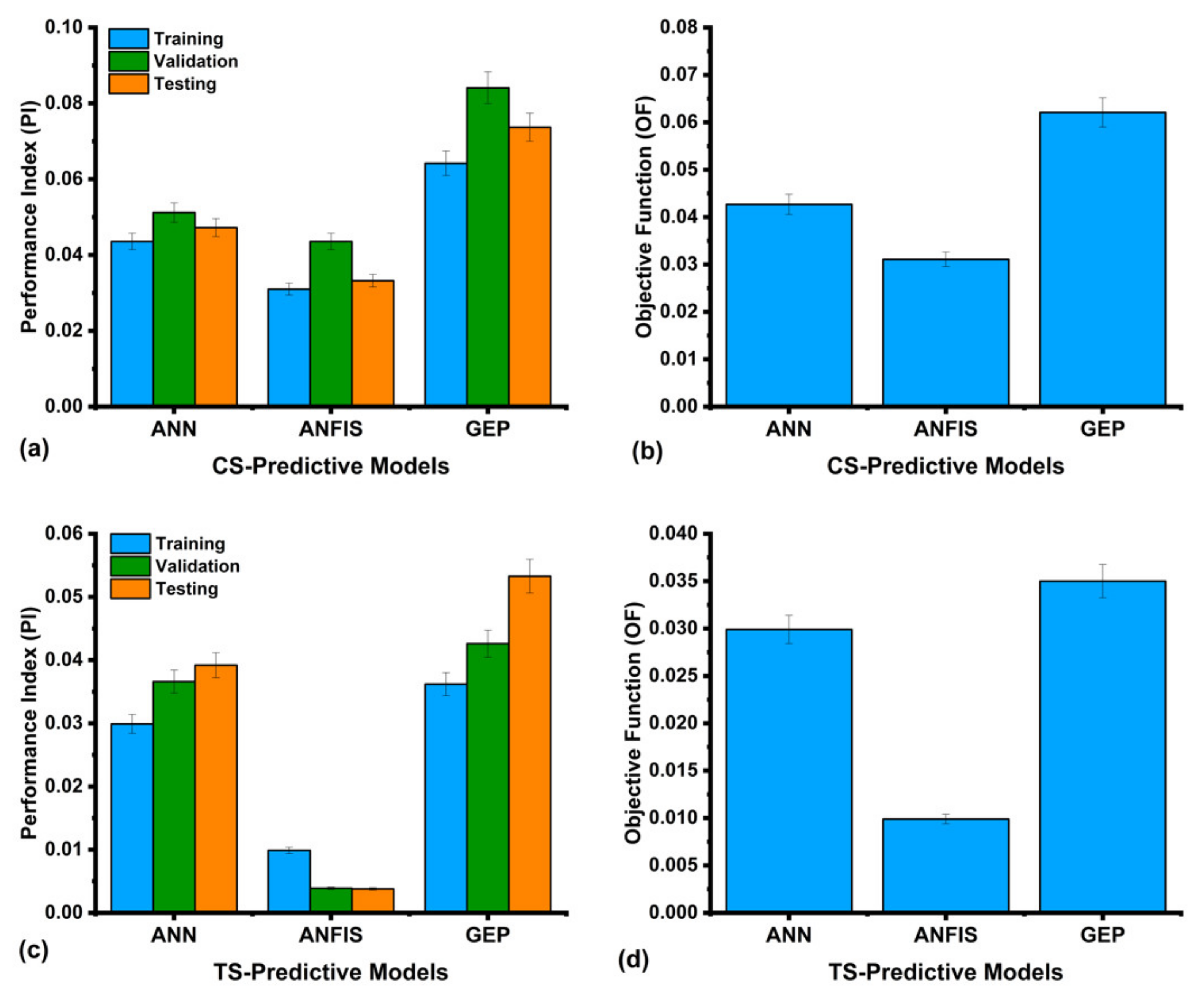
The performance index of the ANN, ANFIS, and GEP models created for CS and TS is less than 0.15, indicating that these models are classified as excellent. Furthermore, it can be noted that the OF values obtained from the ANN, ANFIS, and GEP models for CS are 0.042, 0.031, and 0.062, respectively, and for the TS models, these values are 0.029, 0.009, and 0.035, respectively. The OF values for all cases are close to zero, demonstrating the validity of the proposed models while controlling the overfitting.

(c)

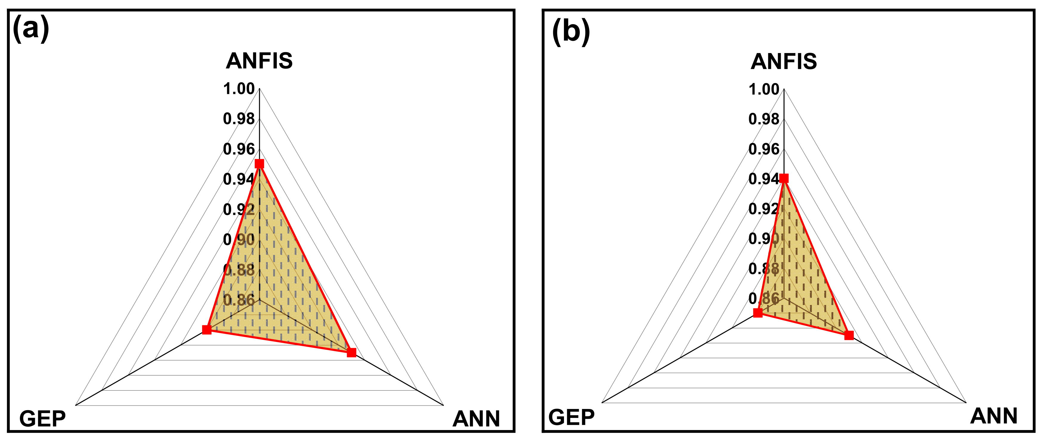
The comparative analysis showed that ANFIS models exhibit higher predictive performance compared to ANN and GEP models. The mean R² values of all three testing conditions (training, testing, and validation) for the CS models are 0.988 (ANFIS), 0.944 (ANN), and 0.887 (GEP), whereas these are 0.998 (ANFIS), 0.954 (ANN), and 0.903 (GEP) for the TS models.

(d)

Based on the MAE values, the ANFIS models showed enhanced performance by 29% and 48%, as compared to the CS models of ANN and GEP, respectively, whereas the ANFIS models for TS showed better predictive performance by 35% and 49% compared to the ANN and GEP models. However, the GEP models showed superior performance compared to the ANFIS and ANNs with respect to the closeness of the statistical measure values between the training, validation, and testing sets for both the CS and TS models.

(e)

GEP is an evolutionary technique that also gives a simple empirical formula for forecasting the CS and TS. This approach significantly diminishes the overall time needed to estimate CS and TS compared with conventional testing procedures, i.e., the evaluation process can be completed at a significantly faster rate. Therefore, the application of the presented equations gives a viable and quick method for the estimation of the CS and TS of concrete containing SF and GGBS.

(f)

External validation based on experimental investigations showed strong evidence for the applicability of the proposed models, with an R² of 0.88 and error percentages of less than 10%.

(g)

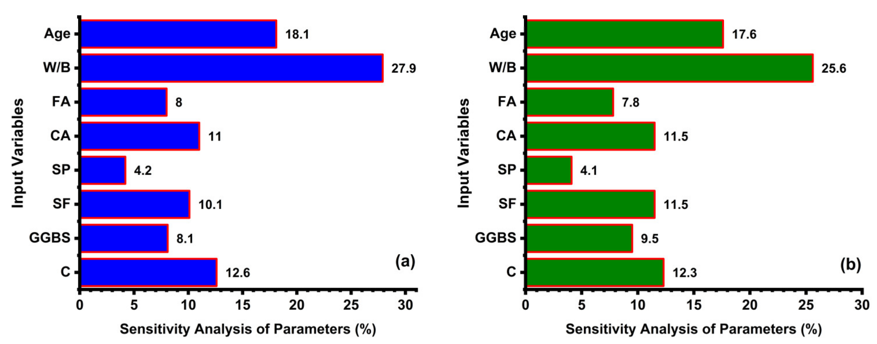
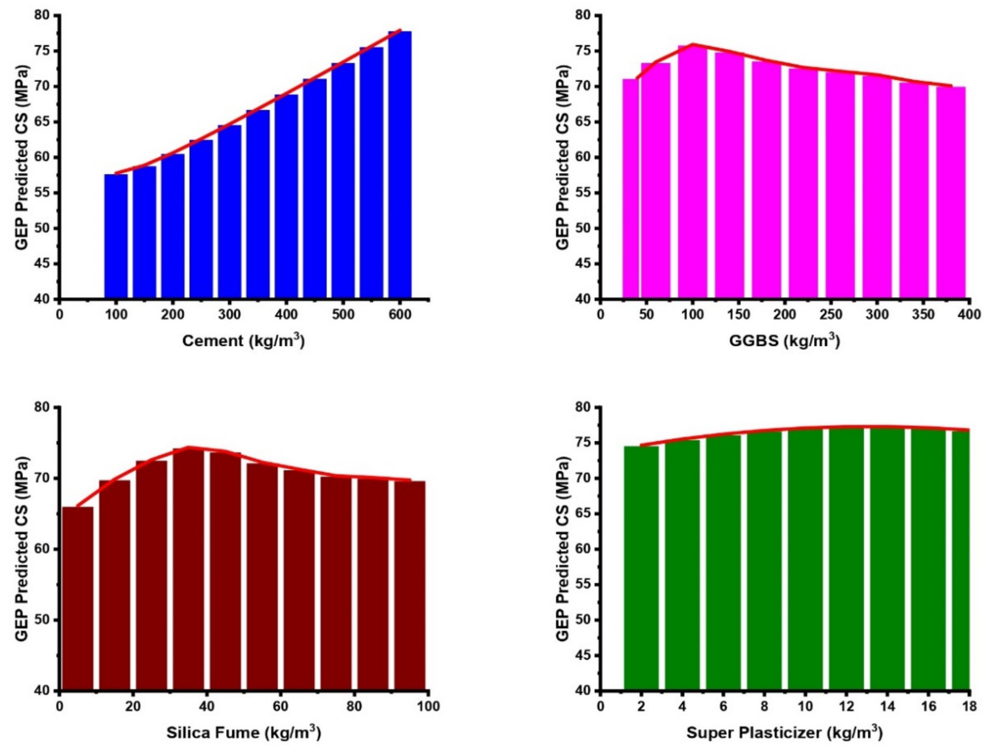
The sensitivity analysis revealed the significance of the input variables to be in the following increasing trend: W/B (27.9%) > age (18.1%) > C (12.6%) > CA (11%) > SF (10.1%) > GGBS (8.1%) > FA (8%) > SP (4.2%) for the CS models, whereas this was W/B (25.6%) > age (17.6%) > C (12.3%) > CA (11.5%) > SF (11.5%) > GGBS (9.5%) > FA (7.8%) > SP (4.1%) in the case of the TS models. These findings are highly comparable with the actual database. The parametric study showed that all of the input variables consistently follow the trend mentioned in the experimental database.

(h)

The developed models successfully fulfilled various criteria that were considered for their external validation.

Finally, it can be deduced that soft computing techniques can provide an efficient basis to promote the utilization of industrial waste in civil engineering applications. The GEP models that have been suggested here have the potential to serve as a standard for forecasting the CS and TS of concrete containing GGBS and SF. Additionally, they may be employed during the initial stages of designing concrete mixes. This can play a key role in sustainable development, as green concrete reduces energy usage, greenhouse gas emissions, disposal, and building costs by using leftover industrial wastes. The findings of this study emphasize the significance of AI techniques as robust and efficient tools for addressing complex challenges in the field of cement-based composites. However, the applicability of the suggested GEP formulations for CS and TS is constrained solely to the range of the input parameters in their corresponding databases. Under this limitation, it is possible to make further adjustments to the existing forecasting models by incorporating an increased number of data points. In addition, the outcomes of this study should be validated by using the increased database for external validation and also by comparing with other machine learning algorithms such as MLPNN, MEP, MLR, DT, SVM, and ensemble methods.

References

1. Arrigoni, A.; Panesar, D.K.; Duhamel, M.; Opher, T.; Saxe, S.; Posen, I.D.; MacLean, H.L. Life cycle greenhouse gas emissions of concrete containing supplementary cementitious materials: Cut-off vs. substitution. J. Clean. Prod. 2020, 263, 121465. [Google Scholar] [CrossRef]
2. Iftikhar, B.; Alih, S.C.; Vafaei, M.; Ali, M.; Javed, M.F.; Asif, U.; Ismail, M.; Umer, M.; Gamil, Y.; Amran, M. Experimental study on the eco-friendly plastic-sand paver blocks by utilising plastic waste and basalt fibers. Heliyon 2023, 9, e17107. [Google Scholar] [CrossRef] [PubMed]
3. IEA: Cement Technology Roadmap 2009–Carbon Emissions Reductions up to 2050. Available online: https://scholar.google.com/scholar_lookup?title=Cement%20Technology%20Roadmap%202009%3A%20Carbon%20Emissions%20Reductions%20up%20to%202050&publication_year=2009&author=IEA (accessed on 17 December 2023).
4. U.S. National Minerals Information Center. Mineral commodity summaries 2020. In Mineral Commodity Summaries; U.S. National Minerals Information Center: Reston, VA, USA, 2020. [Google Scholar] [CrossRef]
5. Global Cement CO2 Emissions 1960–2022 | Statista. Available online: https://www.statista.com/statistics/1299532/carbon-dioxide-emissions-worldwide-cement-manufacturing/ (accessed on 21 March 2024).
6. Cement Production Global 2023 | Statista. Available online: https://www.statista.com/statistics/1087115/global-cement-production-volume/ (accessed on 21 March 2024).
7. Cheng, D.; Reiner, D.M.; Yang, F.; Cui, C.; Meng, J.; Shan, Y.; Liu, Y.; Tao, S.; Guan, D. Projecting future carbon emissions from cement production in developing countries. Nat. Commun. 2023, 14, 8213. [Google Scholar] [CrossRef] [PubMed]
8. Hanifa, M.; Agarwal, R.; Sharma, U.; Thapliyal, P.; Singh, L. A review on CO2 capture and sequestration in the construction industry: Emerging approaches and commercialised technologies. J. CO2 Util. 2023, 67, 102292. [Google Scholar] [CrossRef]
9. Sivakrishna, A.; Adesina, A.; Awoyera, P.O.; Kumar, K.R. “Green concrete: A review of recent developments. Mater. Today Proc. 2019, 27, 54–58. [Google Scholar] [CrossRef]
10. Chen, C.; Xu, R.; Tong, D.; Qin, X.; Cheng, J.; Liu, J.; Zheng, B.; Yan, L.; Zhang, Q. A striking growth of CO2 emissions from the global cement industry driven by new facilities in emerging countries A striking growth of CO2 emissions from the global cement industry driven by new facilities in emerging countries. Environ. Res. Lett. 2022, 17, 044007. [Google Scholar] [CrossRef]
11. Kaish, A.B.M.A.; Odimegwu, T.C.; Zakaria, I.; Abood, M.M. Effects of different industrial waste materials as partial replacement of fine aggregate on strength and microstructure properties of concrete. J. Build. Eng. 2020, 35, 102092. [Google Scholar] [CrossRef]
12. Bheel, N.; Ibrahim, M.H.W.; Adesina, A.; Kennedy, C.; Shar, I.A. Mechanical performance of concrete incorporating wheat straw ash as partial replacement of cement. J. Build. Pathol. Rehabil. 2020, 6, 4. [Google Scholar] [CrossRef]
13. A Elahi, M.; Shearer, C.R.; Reza, A.N.R.; Saha, A.K.; Khan, N.N.; Hossain, M.; Sarker, P.K. Improving the sulfate attack resistance of concrete by using supplementary cementitious materials (SCMs): A review. Constr. Build. Mater. 2021, 281, 122628. [Google Scholar] [CrossRef]
14. Jhatial, A.A.; Nováková, I.; Gjerløw, E. A Review on Emerging Cementitious Materials, Reactivity Evaluation and Treatment Methods. Buildings 2023, 13, 526. [Google Scholar] [CrossRef]
15. Snellings, R.; Suraneni, P.; Skibsted, J. Future and emerging supplementary cementitious materials. Cem. Concr. Res. 2023, 171, 107199. [Google Scholar] [CrossRef]
16. Ahmad, W.; Ahmad, A.; Ostrowski, K.A.; Aslam, F.; Joyklad, P.; Zajdel, P. Sustainable approach of using sugarcane bagasse ash in cement-based composites: A systematic review. Case Stud. Constr. Mater. 2021, 15, e00698. [Google Scholar] [CrossRef]
17. Paris, J.M.; Roessler, J.G.; Ferraro, C.C.; Deford, H.D.; Townsend, T.G. A review of waste products utilized as supplements to Portland cement in concrete. J. Clean. Prod. 2016, 121, 1–18. [Google Scholar] [CrossRef]
18. Piatak, N.M.; Parsons, M.B.; Seal, R.R. Characteristics and environmental aspects of slag: A review. Appl. Geochem. 2015, 57, 236–266. [Google Scholar] [CrossRef]
19. Gupta, S.; Chaudhary, S. State of the art review on supplementary cementitious materials in India—II: Characteristics of SCMs, effect on concrete and environmental impact. J. Clean. Prod. 2022, 357, 131945. [Google Scholar] [CrossRef]
20. Akhtar, M.N.; Jameel, M.; Ibrahim, Z.; Bunnori, N.M. Incorporation of recycled aggregates and silica fume in concrete: An environmental savior-a systematic review. J. Mater. Res. Technol. 2022, 20, 4525–4544. [Google Scholar] [CrossRef]
21. Özbay, E.; Erdemir, M.; Durmuş, H.I. Utilization and efficiency of ground granulated blast furnace slag on concrete properties—A review. Constr. Build. Mater. 2016, 105, 423–434. [Google Scholar] [CrossRef]
22. Gholampour, A.; Gandomi, A.H.; Ozbakkaloglu, T. New formulations for mechanical properties of recycled aggregate concrete using gene expression programming. Constr. Build. Mater. 2017, 130, 122–145. [Google Scholar] [CrossRef]
23. Nafees, A.; Javed, M.F.; Khan, S.; Nazir, K.; Farooq, F.; Aslam, F.; Musarat, M.A.; Vatin, N.I. Predictive Modeling of Mechanical Properties of Silica Fume-Based Green Concrete Using Artificial Intelligence Approaches: MLPNN, ANFIS, and GEP. Materials 2021, 14, 7531. [Google Scholar] [CrossRef]
24. Sun, J.; Zhang, J.; Gu, Y.; Huang, Y.; Sun, Y.; Ma, G. Prediction of permeability and unconfined compressive strength of pervious concrete using evolved support vector regression. Constr. Build. Mater. 2019, 207, 440–449. [Google Scholar] [CrossRef]
25. Farooq, F.; Czarnecki, S.; Niewiadomski, P.; Aslam, F.; Alabduljabbar, H.; Ostrowski, K.A.; Śliwa-Wieczorek, K.; Nowobilski, T.; Malazdrewicz, S. A Comparative Study for the Prediction of the Compressive Strength of Self-Compacting Concrete Modified with Fly Ash. Materials 2021, 14, 4934. [Google Scholar] [CrossRef] [PubMed]
26. Moein, M.M.; Saradar, A.; Rahmati, K.; Mousavinejad, S.H.G.; Bristow, J.; Aramali, V.; Karakouzian, M. Predictive models for concrete properties using machine learning and deep learning approaches: A review. J. Build. Eng. 2023, 63, 105444. [Google Scholar] [CrossRef]
27. Iqbal, M.F.; Javed, M.F.; Rauf, M.; Azim, I.; Ashraf, M.; Yang, J.; Liu, Q.-F. Sustainable utilization of foundry waste: Forecasting mechanical properties of foundry sand based concrete using multi-expression programming. Sci. Total Environ. 2021, 780, 146524. [Google Scholar] [CrossRef]
28. Shahmansouri, A.A.; Yazdani, M.; Ghanbari, S.; Bengar, H.A.; Jafari, A.; Ghatte, H.F. Artificial neural network model to predict the compressive strength of eco-friendly geopolymer concrete incorporating silica fume and natural zeolite. J. Clean. Prod. 2021, 279, 123697. [Google Scholar] [CrossRef]
29. Amlashi, A.T.; Abdollahi, S.M.; Goodarzi, S.; Ghanizadeh, A.R. Soft computing based formulations for slump, compressive strength, and elastic modulus of bentonite plastic concrete. J. Clean. Prod. 2019, 230, 1197–1216. [Google Scholar] [CrossRef]
30. Mahesh, R.R.; Sathyan, D. Modelling the hardened properties of steel fiber reinforced concrete using ANN. Mater. Today Proc. 2022, 49, 2081–2089. [Google Scholar] [CrossRef]
31. Topçu, I.B.; Saridemir, M. Prediction of mechanical properties of recycled aggregate concretes containing silica fume using artificial neural networks and fuzzy logic. Comput. Mater. Sci. 2008, 42, 74–82. [Google Scholar] [CrossRef]
32. Van Dao, D.; Ly, H.B.; Trinh, S.H.; Le, T.T.; Pham, B.T. Artificial Intelligence Approaches for Prediction of Compressive Strength of Geopolymer Concrete. Materials 2019, 12, 983. [Google Scholar] [CrossRef] [PubMed]
33. Sadowski, Ł.; Piechówka-Mielnik, M.; Widziszowski, T.; Gardynik, A.; Mackiewicz, S. Hybrid ultrasonic-neural prediction of the compressive strength of environmentally friendly concrete screeds with high volume of waste quartz mineral dust. J. Clean. Prod. 2019, 212, 727–740. [Google Scholar] [CrossRef]
34. Sebaaly, H.; Varma, S.; Maina, J.W. Optimizing asphalt mix design process using artificial neural network and genetic algorithm. Constr. Build. Mater. 2018, 168, 660–670. [Google Scholar] [CrossRef]
35. Mohammadzadeh: Prediction of Compression Index of Fine-Grained Soils Using a Gene Expression Programming Model. Available online: https://scholar.google.com/scholar_lookup?title=Prediction%20of%20compression%20index%20of%20fine-grained%20soils%20using%20a%20gene%20expression%20programming%20model&author=S.%20Mohammadzadeh&publication_year=2019 (accessed on 12 June 2023).
36. Gandomi, A.H.; Alavi, A.H. Multi-stage genetic programming: A new strategy to nonlinear system modeling. Inf. Sci. 2011, 181, 5227–5239. [Google Scholar] [CrossRef]
37. Awoyera, P.O.; Kirgiz, M.S.; Viloria, A.; Ovallos-Gazabon, D. Estimating strength properties of geopolymer self-compacting concrete using machine learning techniques. J. Mater. Res. Technol. 2020, 9, 9016–9028. [Google Scholar] [CrossRef]
38. Shahmansouri, A.A.; Bengar, H.A.; Ghanbari, S. Compressive strength prediction of eco-efficient GGBS-based geopolymer concrete using GEP method. J. Build. Eng. 2020, 31, 101326. [Google Scholar] [CrossRef]
39. Park, S.; Wu, S.; Liu, Z.; Pyo, S. The role of supplementary cementitious materials (Scms) in ultra high performance concrete (uhpc): A review. Materials 2021, 14, 1472. [Google Scholar] [CrossRef] [PubMed]
40. Balakrishna, Y.; Lavanya, V.; Naresh, A.; Reddy, S.B. Triple Blending of Cement Concrete with Micro Silica and Ground Granulated Blast Furnace Slag. 2016. Available online: www.irjet.net (accessed on 18 February 2024).
41. Akram, M.R.; Raza, S. Effect of Micro Silica and GGBS on Compressive Strength and Permeability of Impervious Concrete as a Cement Replacement. Eur. Acad. Res. 2015, 3, 7456–7468. [Google Scholar]
42. Rajagopalan, G.; Komarasamy, C. Influence of Silica Fume on Strength Characteristics of High Strength Concrete Influence of Silica Fume on Strength Characteristics of High Strength Concrete. Int. J. Earth Sci. Eng. 2018, 6, 2. [Google Scholar]
43. Reddy, K.A.; Kode, V.R.; Malasani, P.; Satish, S.; Darapu, K. Influence of Addition of Micro Silica on Strength Properties of Basalt Fiber Reinforced Multi Blended Concrete. Int. J. Eng. Adv. Technol. (IJEAT) 2019, 9, 4463–4467. [Google Scholar] [CrossRef]
44. Vivek, S.S.; Dhinakaran, G. Engineering Science and Technology, an International Journal Fresh and hardened properties of binary blend high strength self compacting concrete. Eng. Sci. Technol. Int. J. 2017, 20, 1173–1179. [Google Scholar] [CrossRef]
45. Rajeshwari, R.; Mandal, S. Prediction of compressive strength of high-volume fly ash concrete using artificial neural network. Lect. Notes Civ. Eng. 2019, 25, 471–483. [Google Scholar] [CrossRef]
46. Suda, V.B.R.; Paul, S.P. Relationship between compressive, split tensile and flexural strengths of ternary blended concrete. Mater. Today Proc. 2022, 65, 1112–1119. [Google Scholar] [CrossRef]
47. Reddy, S.V.B.; Mounika, P.R. Strength and Durability Studies of Ternary Concrete. J. Appl. Eng. 2018, 13, 12161–12177. Available online: https://www.ripublication.com/ijaer18/ijaerv13n15_65.pdf (accessed on 18 February 2024).
48. Siddique, R.; Kaur, D. Properties of concrete containing ground granulated blast furnace slag (GGBFS) at elevated temperatures. J. Adv. Res. 2012, 3, 45–51. [Google Scholar] [CrossRef]
49. Babu, A. Study on the Strength and Durability Properties of Ternary Blended Concrete. Int. J. Eng. Res. Technol. (IJERT) 2016, 3, 155–160. [Google Scholar]
50. Marani, A.; Jamali, A.; Nehdi, M.L. Predicting Ultra-High-Performance Concrete Compressive Strength Using Tabular Generative Adversarial Networks. Materials 2020, 13, 4757. [Google Scholar] [CrossRef] [PubMed]
51. Haroon, W.; Ahmad, N.; Akram, R.R. Developing of Impervious Concrete Using Silica Fume and GGBS as CEMENT Replacement Materials Department of Civil Engineering. Ph.D. Thesis, University of Engineering and Technology, Taxila, Pakistan, 2012. [Google Scholar]
52. Zhang, W.; Ba, H. Effect of ground granulated blast-furnace slag (GGBFS) and silica fume (SF) on chloride migration through concrete subjected to repeated loading. Sci. China Technol. Sci. 2012, 55, 3102–3108. [Google Scholar] [CrossRef]
53. Juenger, M. Supplementary cementitious materials for concrete: Characterization needs. Mater. Res. Soc. Symp. Proc. 2012, 1488, 106–120. [Google Scholar] [CrossRef]
54. Prakash, S.; Kumar, S.; Biswas, R.; Rai, B. Influence of silica fume and ground granulated blast furnace slag on the engineering properties of ultra-high-performance concrete. Innov. Infrastruct. Solut. 2022, 7, 1–18. [Google Scholar] [CrossRef]
55. Suda, V.B.R.; Rao, P.S. Experimental investigation on optimum usage of Micro silica and GGBS for the strength characteristics of concrete. Mater. Today Proc. 2020, 27, 805–811. [Google Scholar] [CrossRef]
56. Reddy, S.V.B.; Rao, P.S. ScienceDirect Experimental studies on compressive strength of ternary blended concretes at different levels of micro silica and ggbs. Mater. Today Proc. 2016, 3, 3752–3760. [Google Scholar] [CrossRef]
57. Suda, V.B.R.; Rao, P. Influence of Mineral admixtures on Compressive strength of Ternary concrete with different Water binder ratios. IOSR J. Mech. Civ. Eng. 2016, 16, 48–56. [Google Scholar] [CrossRef]
58. Biswal, U.S.; Dinakar, P. A mix design procedure for fly ash and ground granulated blast furnace slag based treated recycled aggregate concrete. Clean Eng. Technol. 2021, 5, 100314. [Google Scholar] [CrossRef]
59. Chandini, S.; Mohammed, P.; Nusari, S. Green Concrete—A Low Cost and Sustainable Solution for a Better Environment. Indian J. Econ. Bus. 2020, 19, 261–269. [Google Scholar]
60. Kumar, S.; Joon, P. A Ternary Blended Concrete Mix with Partial Replacement of OPC with GGBS & Micro Silica and Their Effects on Strength-An Experimental Study Post Graduate Student (Structural Design). 2016. Available online: www.iaster.com (accessed on 18 February 2024).
61. Ghassemzadeh, F.; Shekarchi, M.; Sajedi, S.; Khanzadeh, M.; Sadati, S. Effect of silica fume and GGBS on shrinkage in the high performance concrete. In Concrete under Severe Conditions: Environment and Loading; Taylor & Francis: Abingdon, UK, 2010; Volume 2, pp. 1007–1012. [Google Scholar]
62. Duval, R.; Kadri, E.H. Influence of Silica Fume on the Workability and the Compressive Strength of High-Performance Concretes. Cem. Concr. Res. 1998, 28, 533–547. [Google Scholar] [CrossRef]
63. Mardani-Aghabaglou, A.; Bayqra, S.H.; Nobakhtjoo, A. Specimen size and shape effects on strength of concrete in the absence and presence of steel fibers. Rev. Constr. 2021, 20, 128–144. [Google Scholar] [CrossRef]
64. Elwell, D.J.; Fu, G. Compression testing of concrete: Cylinders vs. cube. Spec. Rep. 1995, 119, 21. [Google Scholar]
65. Gandomi, A.H.; Roke, D.A. Assessment of artificial neural network and genetic programming as predictive tools. Adv. Eng. Softw. 2015, 88, 63–72. [Google Scholar] [CrossRef]
66. Atkinson, A.C.; Riani, M.; Cerioli, A. The forward search: Theory and data analysis. J. Korean Stat. Soc. 2010, 39, 117–134. [Google Scholar] [CrossRef]
67. Khan, S.I.; Hoque, A.S.M.L. SICE: An improved missing data imputation technique. J. Big Data 2020, 7, 1–21. [Google Scholar] [CrossRef]
68. Sharma, C.; Ojha, C.S.P. Statistical Parameters of Hydrometeorological Variables: Standard Deviation, SNR, Skewness and Kurtosis. Lect. Notes Civ. Eng. 2020, 39, 59–70. [Google Scholar] [CrossRef]
69. Brown, S.C.; Greene, J.A. The wisdom development scale: Translating the conceptual to the concrete. J. Coll. Stud. Dev. 2006, 47, 1–19. [Google Scholar] [CrossRef]
70. GN Smith—Probability & Statistics in Civil Engineering PDF | PDF | Matrix (Mathematics) | Normal Distribution. Available online: https://www.scribd.com/document/338933868/GN-Smith-Probability-Statistics-in-Civil-Engineering-pdf# (accessed on 31 May 2023).
71. Pitts, W.; McCulloch, W.S. How we know universals the perception of auditory and visual forms. Bull. Math. Biol. 1947, 9, 127–147. [Google Scholar] [CrossRef]
72. Kourgialas, N.N.; Dokou, Z.; Karatzas, G.P. Statistical analysis and ANN modeling for predicting hydrological extremes under climate change scenarios: The example of a small Mediterranean agro-watershed. J. Environ. Manag. 2015, 154, 86–101. [Google Scholar] [CrossRef] [PubMed]
73. Koçak, Y.; Şiray, G.Ü. New activation functions for single layer feedforward neural network. Expert. Syst. Appl. 2020, 164, 113977. [Google Scholar] [CrossRef]
74. Ramachandran, P.; Zoph, B.; Le, Q.V. Searching for activation functions. In Proceedings of the 6th International Conference on Learning Representations, ICLR 2018—Workshop Track Proceedings, Vancouver, BC, Canada, 30 April–3 May 2018. [Google Scholar]
75. Babu, K.V.N.; Edla, D.R. New Algebraic Activation Function for Multi-Layered Feed Forward Neural Networks. IETE J. Res. 2016, 63, 71–79. [Google Scholar] [CrossRef]
76. Das, S.K. Artificial Neural Networks in Geotechnical Engineering: Modeling and Application Issues. Metaheuristics Water Geotech. Transp. Eng. 2013, 45, 231–270. [Google Scholar] [CrossRef]
77. Tahani, M.; Vakili, M.; Khosrojerdi, S. Experimental evaluation and ANN modeling of thermal conductivity of graphene oxide nanoplatelets/deionized water nanofluid. Int. Commun. Heat. Mass. Transf. 2016, 76, 358–365. [Google Scholar] [CrossRef]
78. Khan, S.; Khan, M.A.; Zafar, A.; Javed, M.F.; Aslam, F.; Musarat, M.A.; Vatin, N.I. Predicting the Ultimate Axial Capacity of Uniaxially Loaded CFST Columns Using Multiphysics Artificial Intelligence. Materials 2021, 15, 39. [Google Scholar] [CrossRef] [PubMed]
79. Moayedi, H.; Mosavi, A. A water cycle-based error minimization technique in predicting the bearing capacity of shallow foundation. Eng. Comput. 2021, 38, 3993–4006. [Google Scholar] [CrossRef]
80. Golafshani, E.M.; Behnood, A.; Arashpour, M. Predicting the compressive strength of normal and High-Performance Concretes using ANN and ANFIS hybridized with Grey Wolf Optimizer. Constr. Build. Mater. 2019, 232, 117266. [Google Scholar] [CrossRef]
81. Islam, M.R.; Jaafar, W.Z.W.; Hin, L.S.; Osman, N.; Hossain, A.; Mohd, N.S. Development of an intelligent system based on ANFIS model for predicting soil erosion. Environ. Earth Sci. 2018, 77, 186. [Google Scholar] [CrossRef]
82. Gene Expression Programming: Mathematical Modeling by an Artificial Intelligence—Candida Ferreira—Google Books. Available online: https://books.google.kz/books?hl=en&lr=&id=NkG7BQAAQBAJ&oi=fnd&pg=PR7&ots=Y_orvEYgF2&sig=nbBd7c2pns60WPMczu9EAjAjPQA&redir_esc=y#v=onepage&q&f=false (accessed on 9 October 2022).
83. Saridemir, M. Genetic programming approach for prediction of compressive strength of concretes containing rice husk ash. Constr. Build. Mater. 2010, 24, 1911–1919. [Google Scholar] [CrossRef]
84. A GENE EXPRESSION PROGRAMMING SYSTEM FOR TIME SERIES MODELING. Available online: https://www.researchgate.net/publication/253404813_A_GENE_EXPRESSION_PROGRAMMING_SYSTEM_FOR_TIME_SERIES_MODELING (accessed on 9 October 2022).
85. Jalal, F.E.; Xu, Y.; Iqbal, M.; Javed, M.F.; Jamhiri, B. Predictive modeling of swell-strength of expansive soils using artificial intelligence approaches: ANN, ANFIS and GEP. J. Environ. Manag. 2021, 289, 112420. [Google Scholar] [CrossRef] [PubMed]
86. Venkatesh, K.; Bind, Y.K. ANN and Neuro-Fuzzy Modeling for Shear Strength Characterization of Soils. Proc. Natl. Acad. Sci. India Sect. A—Phys. Sci. 2022, 92, 243–249. [Google Scholar] [CrossRef]
87. Iqbal, M.F.; Liu, Q.-F.; Azim, I.; Zhu, X.; Yang, J.; Javed, M.F.; Rauf, M. Prediction of mechanical properties of green concrete incorporating waste foundry sand based on gene expression programming. J. Hazard. Mater. 2020, 384, 121322. [Google Scholar] [CrossRef] [PubMed]
88. Zhang, W.; Zhang, R.; Wu, C.; Goh, A.T.C.; Lacasse, S.; Liu, Z.; Liu, H. State-of-the-art review of soft computing applications in underground excavations. Geosci. Front. 2020, 11, 1095–1106. [Google Scholar] [CrossRef]
89. Alade, I.O.; Rahman, M.A.A.; Saleh, T.A. Modeling and prediction of the specific heat capacity of Al2 O3/water nanofluids using hybrid genetic algorithm/support vector regression model. Nano-Struct. Nano-Objects 2019, 17, 103–111. [Google Scholar] [CrossRef]
90. Shahin, M.A. Use of evolutionary computing for modelling some complex problems in geotechnical engineering. Geomech. Geoengin. 2014, 10, 109–125. [Google Scholar] [CrossRef]
91. Kareken, G.; Shon, C.-S.; Tukaziban, A.; Kozhageldi, N.; Mardenov, M.; Zhang, D.; Kim, J.R. Geopolymer as a key material to utilize basic oxygen furnace slag (BOFS) as an aggregate. Mater. Today Proc. 2023. [Google Scholar] [CrossRef]
92. Bakhbergen, U.; Shon, C.S.; Zhang, D.; Kim, J.R.; Liu, J. Optimization of mixture parameter for physical and mechanical properties of reactive powder concrete under external sulfate attack using Taguchi method. Constr. Build. Mater. 2022, 352, 129023. [Google Scholar] [CrossRef]
93. Güllü, H.; Fedakar, H.İ. On the prediction of unconfined compressive strength of silty soil stabilized with bottom ash, jute and steel fibers via artificial intelligence. Geomech. Eng. 2017, 12, 441–464. [Google Scholar] [CrossRef]
94. Hakeem, I.Y.; Althoey, F.; Hosen, A. Mechanical and durability performance of ultra-high-performance concrete incorporating SCMs. Constr. Build. Mater. 2022, 359, 129430. [Google Scholar] [CrossRef]
95. ACI Committee 363. ACI PRC-363-10 Report on High-Strength Concrete; American Concrete Institute: Farmington Hills, MI, USA, 2010. [Google Scholar]
96. Golbraikh, A.; Tropsha, A. Beware of q2! J. Mol. Graph. Model. 2002, 20, 269–276. [Google Scholar] [CrossRef] [PubMed]
97. Alavi, A.H.; Ameri, M.; Gandomi, A.H.; Mirzahosseini, M.R. Formulation of flow number of asphalt mixes using a hybrid computational method. Constr. Build. Mater. 2011, 25, 1338–1355. [Google Scholar] [CrossRef]
98. Cyr, M. Influence of supplementary cementitious materials (SCMs) on concrete durability. In Eco-Efficient Concrete; Woodhead Publishing Series in Civil and Structural Engineering: Toulouse, France, 2013; pp. 153–197. [Google Scholar] [CrossRef]
99. Chu, S.H. Effect of paste volume on fresh and hardened properties of concrete. Constr. Build. Mater. 2019, 218, 284–294. [Google Scholar] [CrossRef]
100. Meddah, M.S.; Zitouni, S.; Belâabes, S. Effect of content and particle size distribution of coarse aggregate on the compressive strength of concrete. Constr. Build. Mater. 2010, 24, 505–512. [Google Scholar] [CrossRef]
101. Samad, S.; Shah, A. Role of binary cement including Supplementary Cementitious Material (SCM), in production of environmentally sustainable concrete: A critical review. Int. J. Sustain. Built Environ. 2017, 6, 663–674. [Google Scholar] [CrossRef]
Figure 1. Region-wise annual CO2 from the cement industry [10].
Buildings 14 01091 g001
Figure 2. Flow diagram of the methodology.
Buildings 14 01091 g002
Figure 3. Outlier detection using raincloud plots for the CS database.
Buildings 14 01091 g003
Figure 4. Outlier detection using raincloud plots for the TS database.
Buildings 14 01091 g004
Figure 5. 3D bar charts representing frequency distribution for the CS database. Note: The measuring unit for all input variables is “kg/m3”, except the age, which is measured in days.
Buildings 14 01091 g005
Figure 6. 3D bar charts representing frequency distribution for the TS (MPa) database. Note: The measuring unit for all input variables is “kg/m3”, except the age, which is measured in days.
Buildings 14 01091 g006
Figure 7. Schematic of ANN models with eight input parameters.
Buildings 14 01091 g007
Figure 8. Representation of ANFIS models with the parametric settings considered in this study.
Buildings 14 01091 g008
Figure 9. Representation of the GEP working process, tree structure, crossover process, and mutation process.
Buildings 14 01091 g009
Figure 10. Comparison of experimental and anticipated results using ANN models for (a) CS and (b) TS.
Buildings 14 01091 g010
Figure 11. Absolute error plots for the ANN models: (a) scatter plot for CS, (b) histogram for CS, (c) scatter plot for TS, (d) histogram for TS.
Buildings 14 01091 g011
Figure 12. Comparison of experimental and anticipated results using ANFIS models for (a) CS and (b) TS.
Buildings 14 01091 g012
Figure 13. Absolute error plots for the ANFIS models: (a) scatter plot for CS, (b) histogram for CS, (c) scatter plot for TS, (d) histogram for TS.
Buildings 14 01091 g013
Figure 14. GEP expression tree extracted for CS.
Buildings 14 01091 g014
Figure 15. GEP expression tree extracted for TS.
Buildings 14 01091 g015
Figure 16. Comparison of experimental and anticipated results using GEP for (a) CS and (b) TS.
Buildings 14 01091 g016
Figure 17. Absolute error plots using GEP: (a) scatter plot for CS, (b) histogram for CS, (c) scatter plot for TS, (d) histogram for TS.
Buildings 14 01091 g017
Figure 18. Slump testing results.
Buildings 14 01091 g018
Figure 19. Laboratory-derived CS outcomes.
Buildings 14 01091 g019
Figure 20. Comparison between the experimental and models’ anticipated values for external validation: (a) CS and (b) TS.
Buildings 14 01091 g020
Figure 21. Models’ R2 values based on the experimental dataset: (a) CS and (b) TS.
Buildings 14 01091 g021
Figure 22. The objective function (OF) and performance index (PI) values of the (a,b) CS models and (c,d) TS models.
Buildings 14 01091 g022
Figure 23. Sensitivity analysis outcomes for (a) the CS models and (b) the TS models.
Buildings 14 01091 g023
Figure 24. Parametric analysis of the CS input parameters.
Buildings 14 01091 g024aBuildings 14 01091 g024b
Figure 25. Parametric analysis of the TS input parameters.
Buildings 14 01091 g025aBuildings 14 01091 g025b