Abstract
Large-diameter bored piles can safely transmit loads from structures by skin friction to the surrounding soil strata and end bearing at the bedrock layer, thereby providing a high compressive capacity. High-Strain Dynamic Testing (HSDT) provides a unique alternative technique to traditional Static Load Testing (SLT) for determining the static compressive resistance of the bored piles, considering its quicker performance and significant cost reductions. This article’s main objective is to numerically explore the performance of large-diameter bored piles during the HSDT and to understand their dynamic behavior under an axial compressive impact force. This research is based on testing pile foundations for reinforced concrete mixed-use towers in the coastal zone of New Alamein City, Egypt. The tested pile is a 1.20 m diameter bored pile. Numerical modeling is performed to simulate both the HSDT and the SLT for two piles at the same site. Non-linear axisymmetric finite element modeling is employed to validate both test records and develop some sort of matching between the two tests. As lumped models, the developed numerical models use the signal-matching process, which is conducted by varying and adopting the strength parameters and deformation characteristics of the ground or soil deposit and the soil–pile interface. The predicted load-displacement curves, developed from analyzing dynamic records employing the Modified Unloading Point (MUP) method, are consistent with the field records. The verified non-linear models are utilized to accomplish a comparative parametric analysis to better understand the drop-mass system aspects. The analysis results emphasize the significance of employing adequate impact energy (i.e., dropping height and mass) to move the pile top to a sufficient extent to mobilize its full resistance. However, a longer impact duration, i.e., larger mass, is more effective for achieving a deeper high-strain wave. The impact load should be developed by a larger drop mass with a lower drop height, not a smaller drop mass with a higher drop height. The results also indicate that, for relatively longer piles, the skin friction of the upper layers surrounding the pile shaft is fully mobilized, whereas the skin resistance of the lower layers is not fully mobilized, regarding the stress wave phenomenon effect. Finally, this study’s findings can be employed to develop guidelines and design procedures for the HSDT to be effectively performed on bored piles.
1. Introduction
Piles are capable of effectively providing a high compressive capacity by transmitting the loads of structures to bedrock or soil strata with adequate safety [1]. In general, pile loading tests are performed to derive the pile’s static capacity as an essential aspect of the pile design approach or to ensure post-construction quality control [2,3,4,5,6]. It can be performed using either static or dynamic loading techniques. The most prevalent method for ascertaining the pile ultimate axial static resistance is the Static Load Test (SLT); however, it is time-consuming and could be prohibitively expensive for large-capacity piles [7]. Nevertheless, the pile can be tested dynamically by applying an impulse force to its head, which can allow quicker implementation as well as a cost reduction. There are generally three categories of this type of testing: StatNamic Load Testing, StatRapid Load Testing, and High-Strain Dynamic Load Testing (HSDT) [8].
In the HSDT approach, an axial compressive impulse force (or load) is applied to a pile by dropping a large reaction mass or a hammer. The combined transducers (i.e., acceleration and strain) are attached to the pile top to record the subsequent responses of the strain and acceleration. The HSDT is issued under the fixed designation code D4945 by the American Society for Testing and Materials (ASTM) [9]. In order to carry out the test, this standard provides several procedures. In the testing procedures, the drop mass must be capable of initiating a force that has the ability to cause the pile to adequately settle so as to reach the ultimate pile capacity. In practice, various testing approaches and techniques for interpreting test records are utilized.
The interpretation of the HSDT can be performed either directly or indirectly. The direct method includes analyzing the recorded data of a single blow through simple soil–pile modeling to calculate the pile load-carrying capacity [10]. The Case method [11] utilized by the Pile Driving Analyzer (PDA) is a perfect illustration of the direct approach. On the other hand, signal-matching programs such as TNOWAVE [12], SIMBAT [13], Allnamics, and CAPWAP [14] are used in the indirect method to analyze the recorded data that result from a single or multiple strikes. The CAse Pile Wave Analysis Program (CAPWAP), which is developed according to wave equation theory, is commonly utilized to analyze displacement piles practically [15].
The PDA is utilized with dynamic load testing. It includes a computerized software application for data gathering and interpretation in the field using a simple technique specified via the Case method [16]. This technique is widely implemented along with cast-in-situ pile integrity testing and the HSDT. The PDA is able to assess the pile load-carrying capacity, hammer efficiency, striking stresses, and the integrity of piles. Also, it provides real-time visualization of recorded signals, instantaneous access to additional options, and the computation of results.
The analog acceleration and strain records are transformed by the PDA into velocity and force measurements graphed versus time. The measured velocity signals are transformed into equivalent forces using the impedance Z of the pile (i.e., F = Zv) to provide direct comparison with the recorded force responses on the same plot scale. Utilizing fundamental dynamic modeling, such as the Case method, the pile static capacity is calculated. Alternative editions of the Case method are established but yield disparate pile compressive resistance predictions for the same tested pile [17]. However, this method is regarded as initial field results; thus, additional analysis is needed to accurately estimate the pile static resistance. The interpretation analysis is performed by signal-matching software, i.e., the CAPWAP, to establish a correlation between the dynamic and static resistance results. It conducts the analysis via the elastic wave theory along with signal-matching approaches in order to determine an appropriate solution that incorporates the total soil resistance, static and dynamic soil resistance, soil stiffness, and damping coefficients.
The HSDT is commonly utilized to determine the pile’s compressive static resistance. In this technique, the impact load remains intact for an impact event of around 5 to 20 ms and is implemented by a dropping mass with a weight of at least 1% to 2% of the desired ultimate static resistance of the pile [18]. The test is carried out at the Beginning Of Re-strike (BOR) or the End-Of-Driving (EOD). Due to the relaxation phenomena and soil setup, the first approach is commonly utilized for accuracy [19].
In general, utilizing the CAPWAP technique for the HSDT interpretation analysis represented a good agreement with the field SLT result [17,20,21,22,23]. Nevertheless, the results of the HSDT are completely conservative as a result of the inadequacy of the implemented set per impact, that is, the transferred energy is insufficient to completely mobilize the pile at full resistance. Therefore, the ultimate loads determined from the SLT are significantly greater than those predicted by the HSDT. Even so, the accuracy of the test interpretation data depends mostly on the engineer’s expertise and input variables. Hence, an appropriate process for the data review and software program must be performed to confirm the results prior to giving a final judgment.
Nath [24] and Mabsout and Tassoulas [25] explored the dynamic behavior of piles exposed to axial compressive impact force and accurately modeled the soil conditions utilizing finite element modeling (FEM). Their studies showed that the results derived from the FEM and the wave equation analysis are in good agreement. Feizee [26] performed an axisymmetric non-linear FEM analysis on a pile driven into sand deposits. The input soil parameters are adopted to better match the measured data submitted by the PDA. In the beginning, the recorded and the calculated forces differed at the tested pile tip. Then, the deformation characteristics of the bearing strata around the tip are modified, achieving a good agreement. Furthermore, Fakharian et al. [27] performed a study to compare the results acquired from the CAPWAP under both scenarios, EOD and BOR, as well as the findings obtained from dynamic finite element and finite difference analyses utilizing axisymmetric Plaxis-2D [28] and FLAC-2D [29], respectively. The PDA is utilized to perform dynamic testing on eight concrete-driven piles in clayey soil. The Mohr–Coulomb criterion is defined to model the soil profile. The matching between their research results on the BOR driving condition is good. The derived load-settlement curves of the tested piles utilizing FEM are in good agreement with the SLT as well.
Naveen et al. [30] conducted FEM modeling utilizing Plaxis 2D in order to derive the load-displacement curve for a bored cast-in-situ pile constructed in a residual soil deposit and then match it to the CAPWAP-derived load-settlement curve. The soil composition is formed of two distinct layers of clay and a weak weathered rock layer. The upper layer is simulated utilizing the Mohr–Coulomb failure criterion; in addition, the lower layer is modeled employing the hardening soil model. Two-dimensional axially symmetric non-linear modeling is conducted using triangular elements with 15 nodes. The derived load-settlement curves acquired from the FEM modeling and CAPWAP software are in good agreement. The authors recommended additional research on various characteristics of the HSDT utilized to predict the pile’s ultimate compressive resistance.
Xin Liu et al. [31] present a novel theoretical model that analyzes the dynamic behavior of concrete-filled steel tube (CFST) piles subjected to vertical loads. Axisymmetric elastic continua are used to simulate the soil, inner concrete pile, and outside steel tube, considering both radial and vertical movements. Then, the interface conditions between various materials and certain mathematical methods are provided in order to derive the theoretical solution for the dynamic impedance of CFST piles. The result indicated that as the steel tube thickness and the CFST pile diameter increase, there is a corresponding upward trend in the dynamic stiffness of the pile. Furthermore, the steel tube and concrete column’s modulus contribute to this trend. The authors emphasize that the CFST pile’s radius and the properties of the surrounding soil have the greatest impact on its soil resistance.
In modeling pile load tests, the FEM provides an acceptable solution to a number of complicated conditions; however, a more accurate assessment is necessary for adjusting the various test variables [32]. Moreover, insufficient information is prevailing regarding simulating the dynamic loading test of bored piles and its corresponding calculations. The FEM is employed successfully to simulate pile load testing. Nevertheless, the performance of bored large-diameter piles under the HSDT employing FEM has not received much interest.
The main purposes of the current study are to explore the performance of bored large-diameter piles under the HSDT and to understand their dynamic behavior under the axial compressive impact force employing numerical methods. Numerical models are used to develop appropriate outlines for the execution of adequate HSDT on bored piles and to assess the capability of the HSDT to accurately determine the static resistance of bored piles. For accomplishing these purposes, 2D axially symmetric non-linear models (FEM) are established using Plaxis 2D software (V22.01).
2. Case Study Pile Description
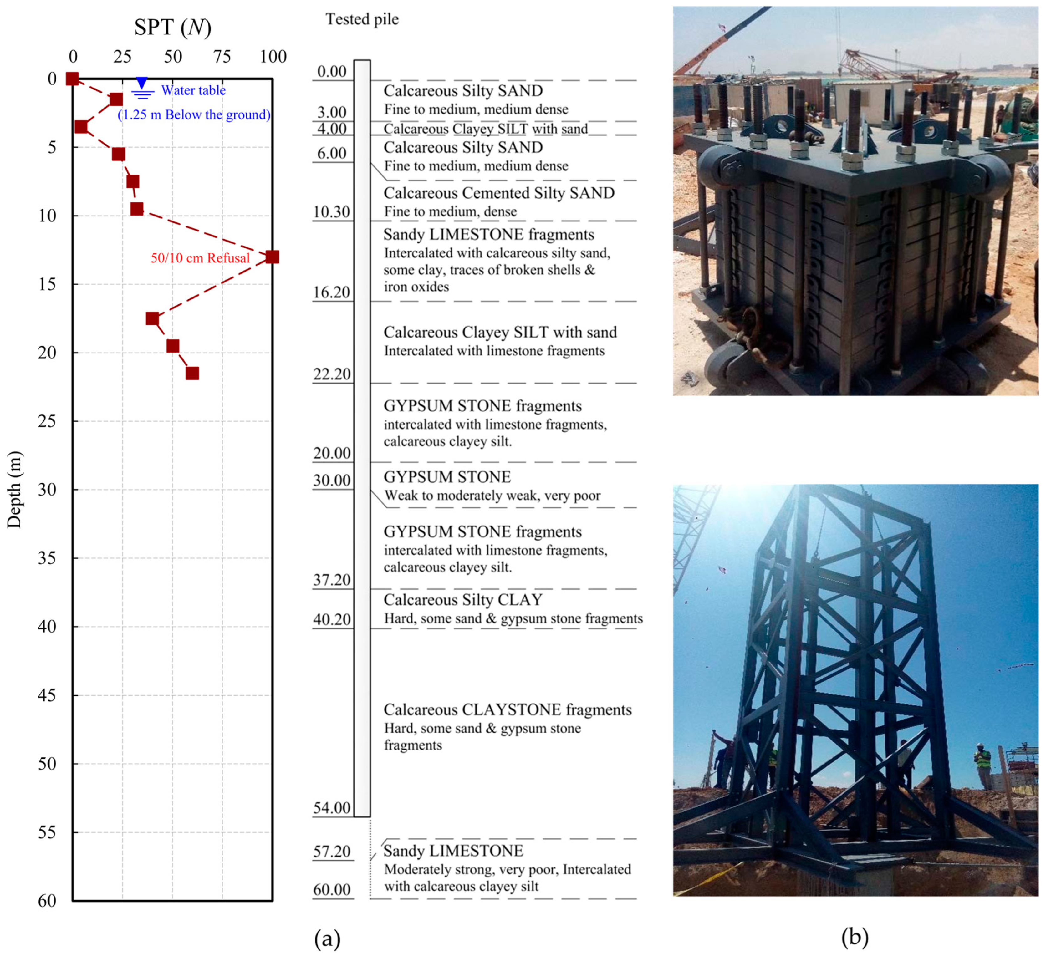
The studied site is located near the shoreline in New Alamein City, North Coast, Matrouh Governorate, Egypt. The proposed project is reinforced concrete mixed-use towers with a height reaching about 150 m, and the studied tower code is LD-04. At the studied site, a total of nine boreholes are drilled to a depth of 60 m. To define the mechanical and physical properties of various soil layers, both disturbed and undisturbed samples are collected, and SPT tests are carried out. Selected unconfined compressive strength tests are conducted on the rock and hard clay samples in order to establish the stress–strain relationship of the tested samples. The unconfined compressive strength and elastic modulus of the studied samples are determined. The provided soil investigation showed that the soil consisted of calcareous silty sand, calcareous clayey silt with sand, sandy limestone fragments, gypsum stone fragments, gypsum stone, calcareous silty clay, calcareous claystone fragments, and sandy limestone layers. The ground water table depth (GWT) is 1.25 m below the ground surface. The SPT N-values and soil profile are shown in Figure 1a according to the borehole (BH.AA04), which is the nearest borehole to the tested bored piles. Furthermore, the bored pile is 54 m long with a diameter of 1.20 m. The HSDT is performed on the bored pile using a free-falling drop-weight system according to ASTM D4945-12 [9], as shown in Figure 1b. Using a PDA-8G, dynamic measurements of the case study are acquired and recorded. The strain transducer attached to the tested pile has a nominal sensitivity of 380 µε/mV/V, the strain range is nominally 3000 µε (functional to 8000 µε), the shock range is nominally 5000 g, and the natural frequency when attached to the pile is greater than 2000 Hz. Furthermore, the accelerometer sensitivity is nominally 1.0 mV/g with a 10 V.D.C. bias voltage input range of 5000 g (limit 10,000 g), and the frequency range is 0.25 to 7000 Hz (resonant frequency: >40 kHz). A signal-matching approach using the CAPWAP software is applied to determine the toe and shaft resistances. The field SLT is conducted according to ASTM D 1143/D 1143M–07 [33] and Egyptian Code of Practice (ECP) for Soil Mechanics and Foundation Design and Construction, 202/4.
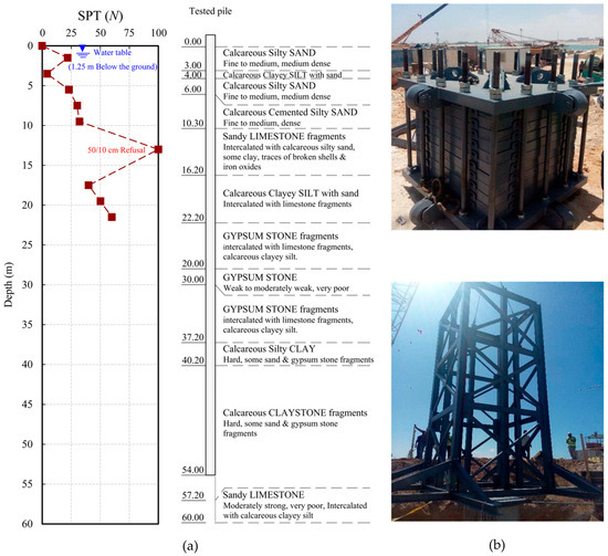
Figure 1.
The studied site. (a) SPT and soil profile at the location of the tested pile. (b) A free-falling drop-weight system is used for HSDT.
3. Analysis Method
The non-linear numerical program Plaxis 2D [28] is employed to conduct sensitive finite element analyses, in which the dynamic behavior of bored piles under dynamic load testing is studied. The numerical models are verified and matched with the case study. The Mohr–Coulomb material model (MC) is defined to model the non-linear soil response of the upper layers. On the other hand, the lower layer at the toe is simulated utilizing the hardening soil model with small-strain stiffness (HS-small). The bored concrete pile is modeled utilizing the linear elastic material model regarding the non-porous drainage type. The verified non-linear models are utilized to accomplish a comparative parametric analysis to understand the drop-mass system aspects that affect the dynamic behavior of bored large-diameter piles during dynamic impact loading.
3.1. Model Geometry and Boundary Conditions
To accurately simulate the response of the soil to static and dynamic impact loading developed by static and dynamic load testing, the model dimensions must be located far enough away from the studied pile to eliminate boundary effects. The recommended model size (L × 2L), according to their studies [27,34,35,36,37], should be used for optimal accuracy and calculating efficiency. Moreover, the model geometry is evaluated by changing the position of the vertical and horizontal boundaries until the calculated responses converge to a constant value at the pile head. Hence, in the horizontal direction, the model geometry is located at the distance L (pile length) from the symmetry axis, and in the vertical direction, it is located at the distance 2L under the ground surface. For SLT modeling, the bottom boundary is constrained. An unconstrained boundary is allocated to the model top, and roller supports should be allocated to the vertical boundaries, thereby restricting horizontal movement. To accurately model the wide-field response of the soil deposit in HSDT modeling, the absorbing boundaries should be adopted to the bottom and side boundaries. To accomplish this, viscous boundaries are assigned that absorb the propagating wave energy generated by the axial compressive impact load, thereby preventing any wave rebound inside the soil strata. In both the x and y directions, viscous dampers are specified at the extreme boundaries by Plaxis 2D.
3.2. Material Model
For both dynamic and static loading simulations, the MC model is defined to characterize the non-linear response of the upper layers. On the other hand, the lower layer at the toe is modeled using the HS-small model. The bored concrete pile is modeled utilizing the linear elastic material model regarding the non-porous drainage type with assigned concrete properties. The unit weight of a bored pile is taken as 24 kN/m3, the modulus of elasticity is set at 29.5 GPa, and the Poisson’s ratio is defined as 0.20. The dynamic modulus of elasticity of the bored concrete pile can be calculated as the product of the mass density times the square of the strain wave propagation speed in the pile material (E = ρ c2) [9,38]. The dynamic modulus of elasticity is taken as 30.11 GPa. Furthermore, in the numerical simulations, the soil deposit and the bored pile interaction are modeled utilizing interface elements, applying the parameter Rinter, specified as the interface reduction factor [39,40]. In accordance with Equations (1)–(3), the Rinter factor accounts for the strength reduction of the interface element within the corresponding soil stratum.
Regarding the used finite element mesh, the load-settlement curve and the predicted velocity–time-response curve at the top of the tested pile are employed as the mesh convergence criterion, considering the computational requirements and accuracy. In the analysis, the option for global refinement mesh is utilized.
3.3. Drainage Condition
Since the dynamic loading rate is higher than the pore water pressure (PWP) dissipating rate, excess PWP is generated, which affects the resistance of the soil. Holeyman [18] specifies that even in sandy soil, faster excess PWP dissipation is restricted by the rate of loading. Hölscher and Barends [41] reported that the developed PWP dissipation time in dense sand strata is significantly longer than the dynamic loading duration of the HSDT. Maeda et al. [42] determined that during the test, the dissipation duration of excess PWP around the tip of the pile is almost 400 ms in saturated sand, considering the soil behavior is undrained. According to the previous discussion, due to the short dynamic loading duration and the soil condition presented in the studied case, undrained analysis is adopted.
3.4. Materials Model Parameters
The MC model under the undrained condition is utilized to simulate the response of the upper surrounding soil layers realistically. The deformation characteristics, including shear modulus (G) and modulus of elasticity (Es) at large-strain and low-strain, are approximated using empirical correlations with the SPT-N values. Moreover, in situ soil description is used to select the most relevant correlations. The empirical correlations of Webb [43], Begemann [44], Papadopoulos [45], and Bowles [46] are applied to adopt the used modulus of elasticity. The average value of these correlations is chosen for each soil layer.
The HS-small is developed from the original hardening soil model, which employs nearly all parameters. The deformation characteristics, including the secant modulus of elasticity (), are estimated using the soil investigation data. In many practical cases, it is appropriate to define = 3, and in engineering practice, = can be assumed, whereas these parameters are referred to as tangent stiffness () and unloading–reloading stiffness () [47]. According to Dung [48], since the MC failure criterion is also utilized for the HS-small model, the MC friction angle and cohesion parameters are also utilized. Additionally, the exponent, m, was used in the hardening soil model to represent the stress-level dependency of the stiffness. Furthermore, only two supplemental stiffness parameters, Go and γ0.7, are required to indicate the shear stiffness–strain relationship. Go is the shear modulus at the initial very small strain, and the threshold shear strain level γ0.7 is the characteristic shear strain at which the secant shear modulus Gs is decreased to almost 70% of Go. During unloading and reloading, the standard hardening soil model indicates elastic material behavior. However, soils can be regarded as purely elastic, in which the characteristic strain range is very small. Increases in the strain amplitude cause a non-linear decrease in the soil stiffness [47].
The HS-small under the undrained condition is used to effectively simulate the response of the bearing soil layer at the pile tip. The dynamic modulus of elasticity is defined to estimate the initial shear modulus (Go) by applying the chart developed by Alpan [49]. Hence, the adopted static soil modulus of elasticity, that is, Edynamic ≈ 2 Estatic. The shear strain (γ0.7) is adopted at 8 × 10⁻⁴ for the calcareous claystone fragment layer (at the pile tip) to assess the impact of the small-strain parameters of the HS-small model on the measured velocity at the transducer location (at the pile head).
The damping ratio of the soil material is needed to depict the dynamic response under the dynamic load event. Assuming a 5% damping ratio, Rayleigh damping is utilized to take into consideration soil damping. The two different target frequencies for estimating the corresponding Rayleigh damping parameters are calculated in accordance with the approach proposed by Hashash and Park [50], i.e.,
where f1 and f2 are the first and second (limit) target frequencies; fd is the dynamic loading predominant frequency; and h and vs are the thickness and shear wave velocity of the soil deposit, correspondingly.
However, there is an additional difficulty in this case study due to the existence of eleven layers above the rigid bedrock. This restriction is solved using the code EERA [51], and then the Rayleigh damping coefficients are calculated utilizing a unique equivalent strata based on rigid bedrock. The average velocity of the shear wave, Vsm, of the equivalent soil deposit is determined as
The equivalent soil deposit fundamental period, T, is specified as
3.5. Input Parameters and Final Geometry Model
The soil profile of the case study is subdivided into twelve layers. Figure 2 indicates the final model geometry generated in Plaxis 2D for the case study, comprising the model dimensions, mesh generation, and pile–soil deposit interaction. The adopted soil parameters utilized for the studied case are depicted in Table 1.
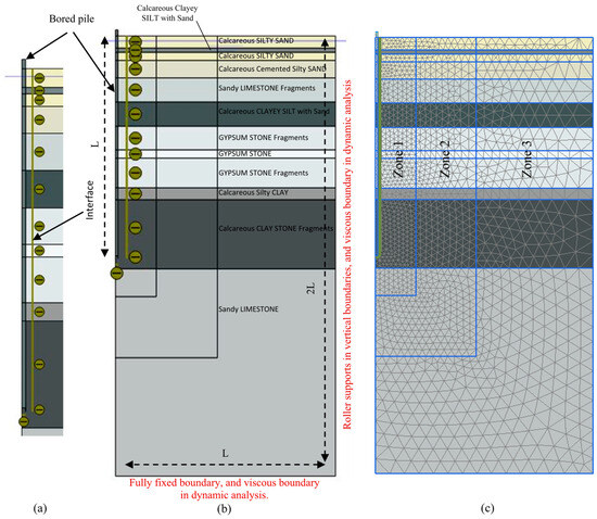
Figure 2.
Case study modeling: (a) bored pile and pile–soil interface, (b) model dimensions, and (c) mesh discretization.

Table 1.
Input parameters defined in the numerical model for the case study.
4. High-Strain Dynamic Testing (HSDT) Numerical Modeling
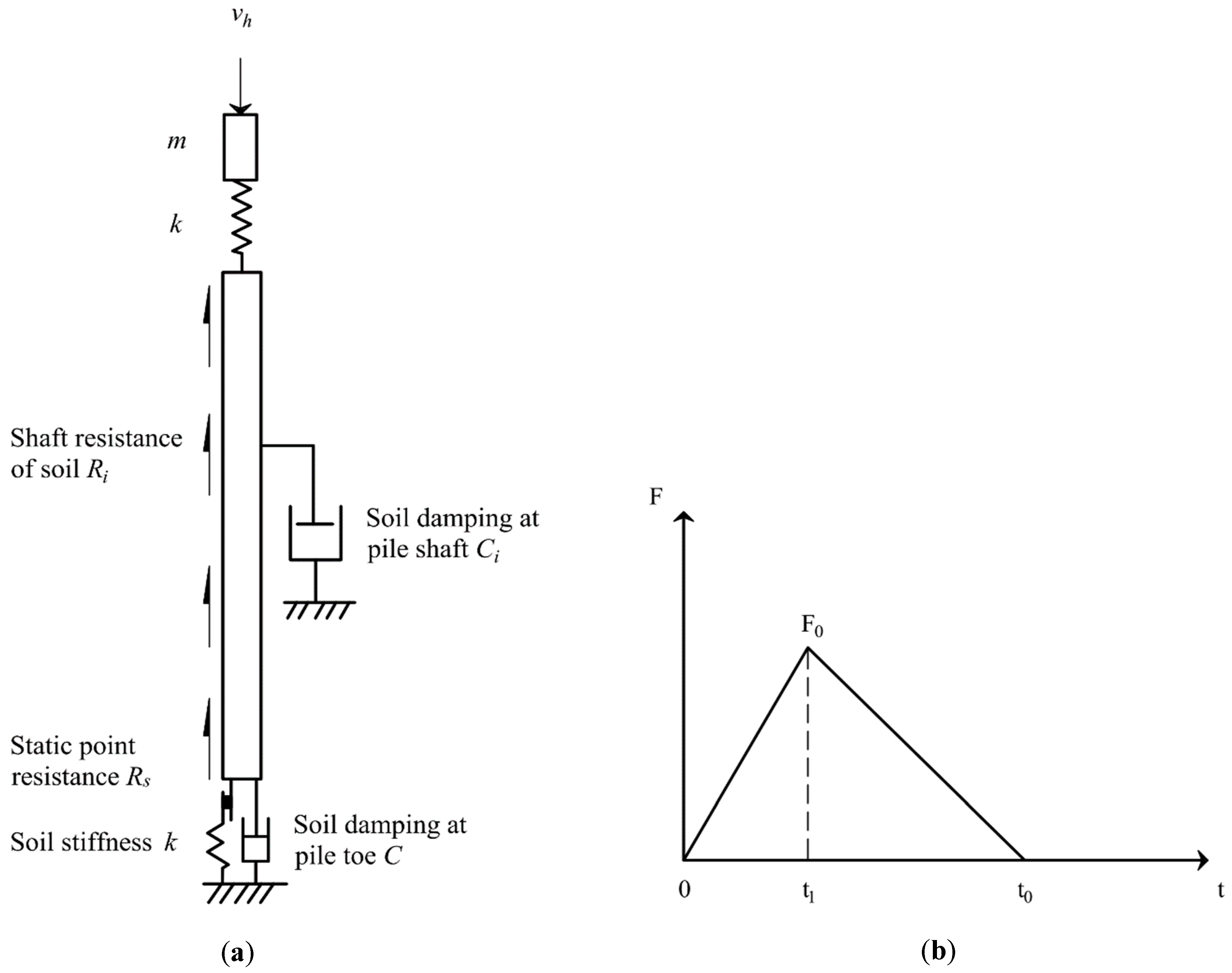
The non-linear time-domain analysis of the dynamic impact loading under the HSDT is performed, simulating the dynamic records (acceleration, velocity, and force responses). The top of the tested bored pile is exposed to an impulse force from the free-falling drop-weight system. The physical model of the dynamic pile hammering developed by Chen et al. [52] (as depicted in Figure 3a) is utilized in this study. Regarding the pile compression, pile cushion stiffness, and other related characteristics, the model can be used to satisfy the requirements of engineering applications [53].
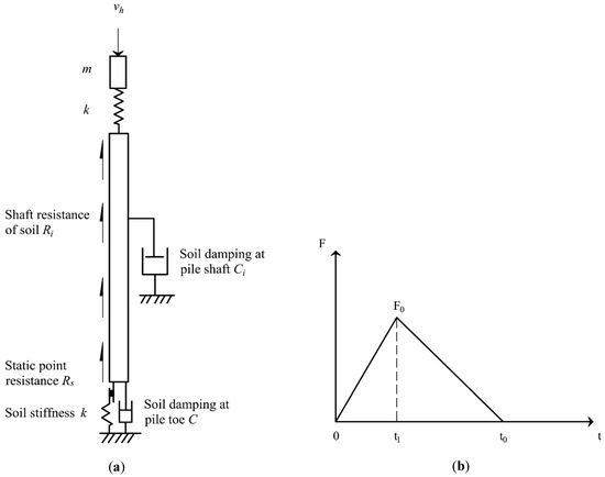
Figure 3.
(a) Physical model of dynamic pile hammering developed by Chen et al. (b) Force–time response of triangular impulse load on the bored pile head.
The impulse load on the head of the pile can be determined through the subsequent equation, based upon the physical model represented in Figure 3a:
In Equation (7), k, νh, and t are the equivalent pile cushion stiffness, the drop-mass impact velocity on the pile cushion, and the elapsed time during impact, respectively; ω, ωd, and ξ are the natural frequency, damped natural frequency, and damping ratio, which control the amplitude of the impact load and shape:
where Lh, Ah, and Eh are the pile cushion material thickness, cross-sectional area, and elastic stiffness, respectively; and g and h are the gravity acceleration and drop height, respectively.
where M, E, and A are the drop mass, elastic modulus, and cross-sectional area, respectively.
The single-impact load shape on the bored pile head resembles a half-sinusoidal function, as shown in Equation (7), where the peak impact force and impact duration are the critical parameters. In addition, variations in the drop mass, impact velocity, cushion stiffness, and other characteristics affect these parameters. As shown in Figure 3b, the force–time-response graph corresponds to the triangular impulse load applied to the bored pile head.
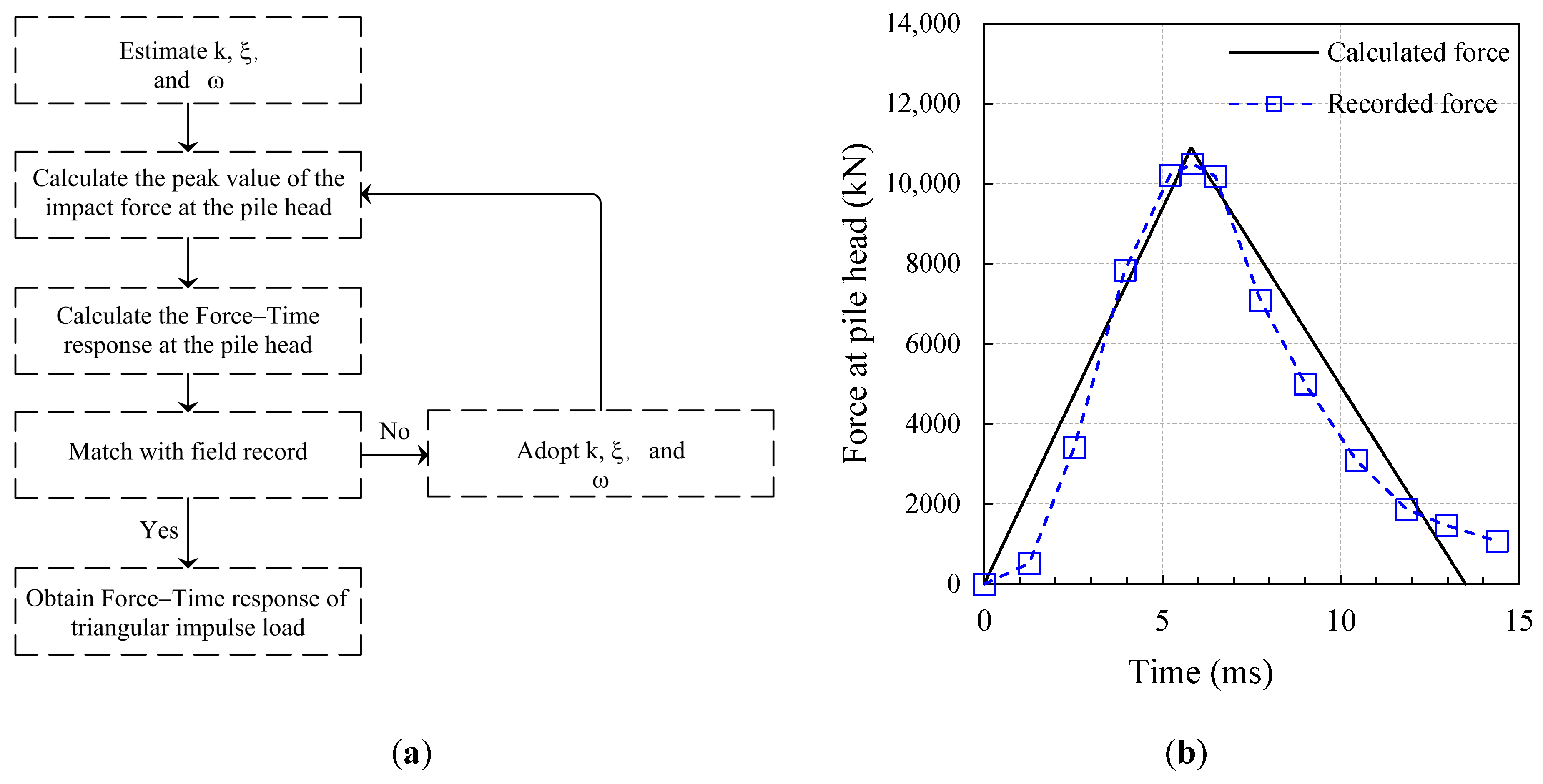
In order to verify Equation (13), initially, the recorded impulse force applied to the head of the pile by the drop-mass impact is graphed versus time. Then, the pile pad stiffness, damping ratio, and pile cushion–drop-mass system frequency are calculated and assessed through Equations (13)–(15) to develop the force–time-response graph of the triangular impulse load on the bored pile head. As these parameters are not reported, therefore, they are correlated from other parameters and updated as a re-match is achieved between the recorded and the predicted responses. Figure 4a is a flowchart that summarizes the procedure explored to calibrate and validate the derived equations. Significantly, the matching process is established based on the impact duration (t0), the peak value of the impact force (F0), and the peak impact force loading time (t1) [8].
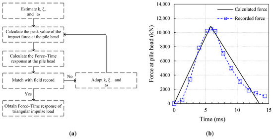
Figure 4.
(a) Flowchart of the verification process of the impact load on the bored pile head. (b) Calculated force response from Equation (15) compared against the recorded force response at the tested bored pile head.
For the tested bored pile, the drop mass is 18 tons and is dropped from a height of 0.60 m. The used pile cushion is made of a variety of materials, including hardwood, masonite fiber plates, and other kinds of man-made materials are used. Figure 4b compares the recorded force–time history at the head of the tested bored pile with the response calculated from Equation (15). As shown in Figure 4b, the estimated force–time history for the tested pile is consistent with the recorded response. The good agreement between the initial and peak values of the impact forces suggests that the system’s damping, equivalent cushion stiffness, and pile impedance are accurately estimated. After the peak value of the impact force, however, the calculated forces did not match exactly the measured field forces in which a slight reduction in the force took place. It means that either the pile top is affected by the impact force or the impedance (Z) of the tested bored pile is non-uniform as a result of the variation in the cross-sectional area of the pile. Consequently, the system damping ratio no longer remains constant. However, an agreement between the calculated and recorded forces is observed in the last portion of the responses as well.
The dynamic time interval, Δt, used in the dynamic calculations is equivalent to the impact time recorded during the real test. The time duration is discretized into m, the maximum step value, and n, the sub-step value. Using the max steps and number of sup-steps parameters, the dynamic time interval is subdivided into the optimal time step to accomplish the impact event.
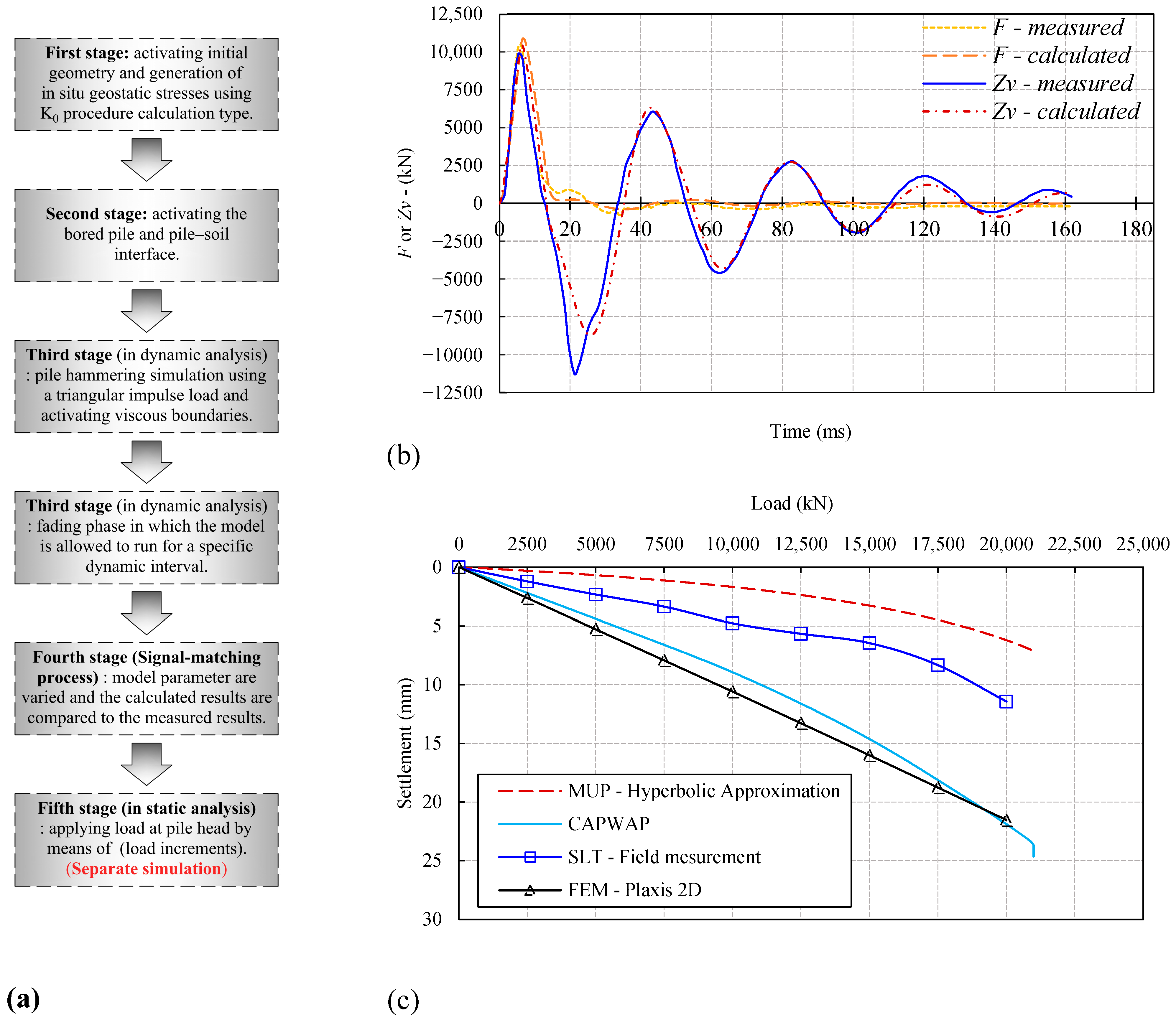
The dynamic analysis is conducted in four stages: the initial phase, the pile creation phase, the pile-striking modeling phase, and the fading phase. The model’s initial stresses and groundwater conditions are calculated in the initial phase using the K0 procedure. The tested pile is activated in the subsequent phase by specifying the concrete material properties for the corresponding volume cluster. During this phase, the interface element is also activated. In the third phase, i.e., dynamic calculations, a single stroke is applied to the tested pile head utilizing a distribution unit load with a dynamic load multiplier. The viscous boundaries are assigned and activated, and the dynamic time interval is set to 0.0135 s. In the final phase, i.e., dynamic calculations, the attenuation of the induced stress wave is noticed. Due to the generated compression stress wave continuing to propagate downward in the bored pile, the maximum settlement occurs during this phase. The dynamic computations are extended for 0.15 s after the dynamic impulse load is deactivated to model the fading of stress wave propagation in the bored pile.
5. Static Load Testing Numerical Modeling
The SLT is modeled using static incremental loads applied to the top of the tested pile. The static analysis is conducted in 11 phases: the initial phase, the pile construction phase, and 9 pile incremental loading phases. The analysis of both the initial and subsequent phases is performed in the same manner as discussed in the preceding section. Moreover, in the second phase, the boundary conditions are adopted for the static loading calculations. In the last nine phases, load increments are applied to the head of the tested pile to model the SLT. The test load is 200% of the pile design capacity. The progressive loading is applied by load increments of 0.0, 2500, 5000, 7500, 10,000, 12,500, 15,000, 17,500, and 20,000 kN at the top of the pile and the calculated settlements for the corresponding loads are plotted. The load-settlement curves, both measured and calculated, are employed in this study to verify the model assumptions.
6. Derived Load-Settlement Curve
The CAPWAP utilizes the PDA system’s dynamic records during the dynamic load test to derive the pile’s static resistance. The CAPWAP is employed by CH2M HILL, Ltd. [54], founded in Corvallis, OR, USA, to establish the calculated resistance-settlement curve. In the same manner, the dynamic responses (i.e., strain, velocity, acceleration, and displacement records) acquired from the numerical model are analyzed employing different approaches to develop the load-settlement curve. The derived static load-settlement curve is developed utilizing two approaches established upon the wave number, Nw = cT/L (T = impulse interval, and L = length of the pile). For Nw > 6, the Unloading Point (UP) approach is utilized [55]. The stress wave phenomena effects become larger for Nw < 10 [56]; therefore, the Modified Unloading Point (MUP) approach developed by Justason [57] should be utilized.
The UP approach emphasizes analyzing the pile–soil system as a Single-Degree-Of-Freedom (SDOF) model, consisting of a linear dashpot and a non-linear spring under transient accelerations and forces [58]. The viscous damping constant (c) represents the dynamic resistance resulting from the penetration rate, while the stiffness coefficient (k) represents the static soil resistance. The UP method is developed based on two fundamental assumptions: firstly, the damping coefficient remains constant during the test, and secondly, the pile is a rigid body. The analysis is performed at the unloading point, defined as the instant where the displacement is at its maximum (velocity is zero); hence, eliminating the damping effect simplifies the equilibrium forces to the static soil resistance, impact force, and inertia force [59]. The load-settlement curve can be accurately described using a hyperbolic model [60]:
where u(t), K0, Fstatic(t), tmax, and η are the pile displacement at time t, initial stiffness calculated from dynamic records, the static response of the soil at time t, time at maximum displacement (and zero velocity), and reduction empirical factor, respectively; a(tmax) and m are the acceleration at maximum displacement and pile mass.
where vmax and I are the maximum velocity calculated through the test and viscosity index.
In the case of relatively longer bored piles, the pile movement at the top can significantly differ from the pile movement at the tip; hence, the assumption that the pile is a rigid body is invalid in such a case. To resolve these instances, a modified method (MUP) based on the UP approach is established. The MUP method requires an additional set of acceleration sensors to detect the dynamic responses at the tip of the pile. This approach assumes that the pile is simulated as an SDOF model; however, the system motion is defined as the mean of the dynamic responses observed at both the pile’s head and tip. These methods’ procedures are discussed in detail elsewhere [57,60,61]. Consequently, the MUP method is employed to analyze the dynamic responses measured from the FEM modeling to derive the calculated load-settlement curve.
7. Verification
In the verification technique, the developed numerical model (FEM-Plaxis 2D) is first validated for performing the dynamic modeling of the HSDT (dynamic response) before conducting the SLT (static response). The dynamic response of the developed numerical model is verified by a signal-matching procedure. A set of parameters is varied and adopted to conduct a signal-matching process, including the soil or ground deposit and soil–pile interface parameters such as the deformation characteristics and shear strength. The adopted parameters, as shown in Table 1, are also assessed and matched to the ground or soil parameters obtained from the site investigation data. Figure 5 summarizes the developed FEM utilized for the study case, including the modeling procedures, results of signal-matching analysis, and load-settlement curve results for both dynamic and static modeling compared against the field records.
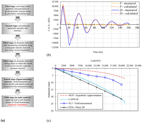
Figure 5.
A summary of the developed FEM for the study case: (a) modeling procedures, (b) signal-matching analysis results, and (c) load-settlement curve results for both dynamic and static modeling compared against field records.
7.1. Signal-Matching Method
The specific parameters used during the signal-matching process are the significant differences in the FEM and the CAPWAP approaches. In the CAPWAP model, the pile shaft resistance (Rs) and the resistance calculated at the tip of the pile (Rt) are varied. However, in the FEM model, the soil deposit shear strength parameters (c and φ) and pile–soil interface strength reduction factor (Rint) are varied instead [27]. These parameters are adopted until a better match is obtained between the predicted and measured waves.
7.2. Results of Signal-Matching Analysis
Figure 6a,b illustrate the average force F(t) and Zv(t) (impedance times velocity) recorded by the attached strain transducers and accelerometer sensors, respectively, at the bored pile head, along with the force F(t) and Zv(t) calculated through numerical analyses utilizing the FEM model. In practice, velocity v(t) is the particle velocity determined by integrating accelerometer records at the top of the pile with respect to time, t. The pile impedance Z (dynamic stiffness) is based upon the material properties and the pile material density, as per Equation (19).
where E, A, and ρ are the dynamic elastic modulus at the sensor cross-section, cross-section area at the sensor level, and density of the pile material, respectively. For the cast-in-situ concrete piles, the elastic wave propagation speed (c) is around 3700 m/s. The force F(t) and Zv(t) responses are compared on the same force–time graph as depicted in Figure 5b, where the velocity is scaled to the force unit. Both the calculated and measured Zv(t) waves are derived from the multiplication of the velocity–time response and the impedance Z. The calculated and measured force–time responses F(t) are developed from the calculated and measured strain ε(t), respectively, at the stress point (FEM) and the strain transducer, both at the same elevation installation at the pile head, using Equation (20).
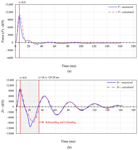
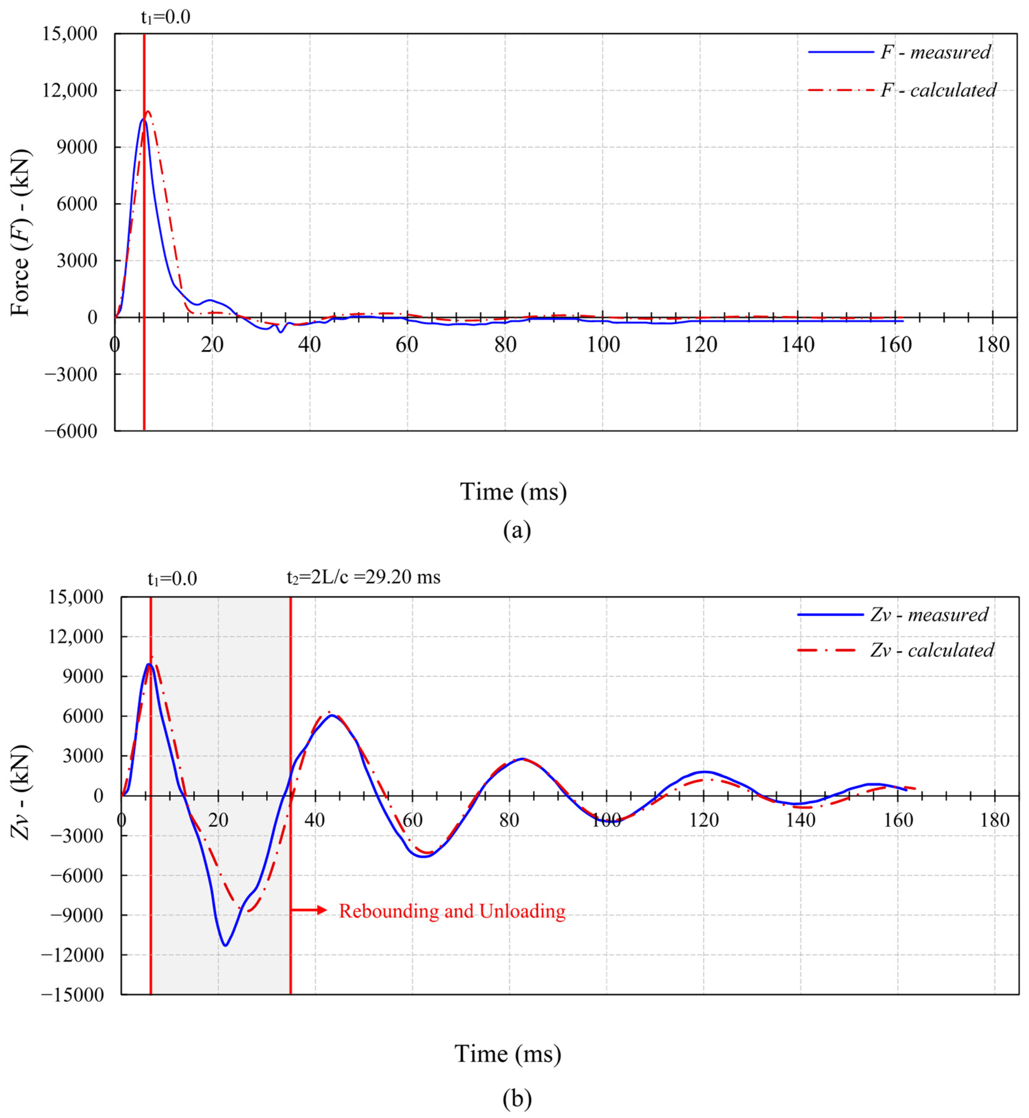
Figure 6.
(a) Measured and calculated force F(t) responses and (b) measured and calculated Zv(t) (velocity times impedance) wave responses.
During the dynamic analysis, the soil deposit and the interface element characteristics of Table 1 are assigned for each stratum. Subsequently, the calculated Zv(t) at the same node (i.e., transducer attachment point) is graphed over time and matched to the recorded Zv(t) values. In order to adapt a better fit between the measured and calculated Zv(t) responses, the following trial-and-error analyses are performed to adopt the interface element and the soil deposit parameters, specifically the bearing layer at the pile tip.
The most significant time interval affecting mobilizing the resistance of the pile shaft starts from the first maximum peak force (or impedance times velocity, Zv) to the toe reflection, or 2L/c (where c is the elastic wave propagation speed and L is the distance from the transducer attachment level to the pile tip), which is 29.2 ms in this case study. The procedure of signal matching is outlined separately for (A) the shaft and (B) the tip of the pile, as follows:
- (A)
- Signal matching along the shaft: the three categories of parameters (i.e., deformation characteristics, damping ratio, and shear strength), as provided inTable 1, are considered through the signal-matching process. The signal-matching trials are conducted through a specific time segment between the first maximum peak force (t = 0) and toe reflection values (t = 2L/c). Moreover, the interface strength reduction factor (Rinter) is adjusted. In the developed (FEM) model, the interface thickness is defined directly by the plaxis software. The interface stiffness is derived from the deformation characteristics of the adjacent soil media at each strata [61]. The shear strength characteristics of the soil media are varied until the calculated Zv(t) matches the measured Zv(t) reasonably well between the maximum peak force and toe reflex values.
- (B)
- Signal matching around the pile toe: in the developed FEM model, the deformation characteristics, shear strength, and small-strain parameters (dynamic soil stiffness) of the soil deposit around and below the pile toe are varied for signal-matching objectives.
Figure 6a discusses the force F(t) calculated by the FEM, which shows a reasonable match with the field records. In the impact peak (t = 0) observed in the force response F(t), the calculated F is equal to 10,893 kN, which corresponds to an excellent match against the measured F value of 10,610 kN. Figure 6b illustrates the velocity times impedance Zv(t) predicted by the FEM, indicating a reasonable agreement with the field records during the dynamic loading and fading phases. For instance, in the initial impact peak (t = 0) detected in the velocity times impedance response Zv(t), the Zv is predicted to be 10,356 kN, which also agrees well with the recorded Zv of 9862 kN. In the time coinciding with the wave reflection (t = 2L/c), the calculated and measured Zv are −116 kN and 812 kN, respectively, confirming the ability of the proposed numerical model and procedure to evaluate the high-strain dynamic testing utilizing the finite element approach.
7.3. Load-Settlement Curve Results for Both Dynamic and Static Modeling (FEM) Compared against Field Measurements
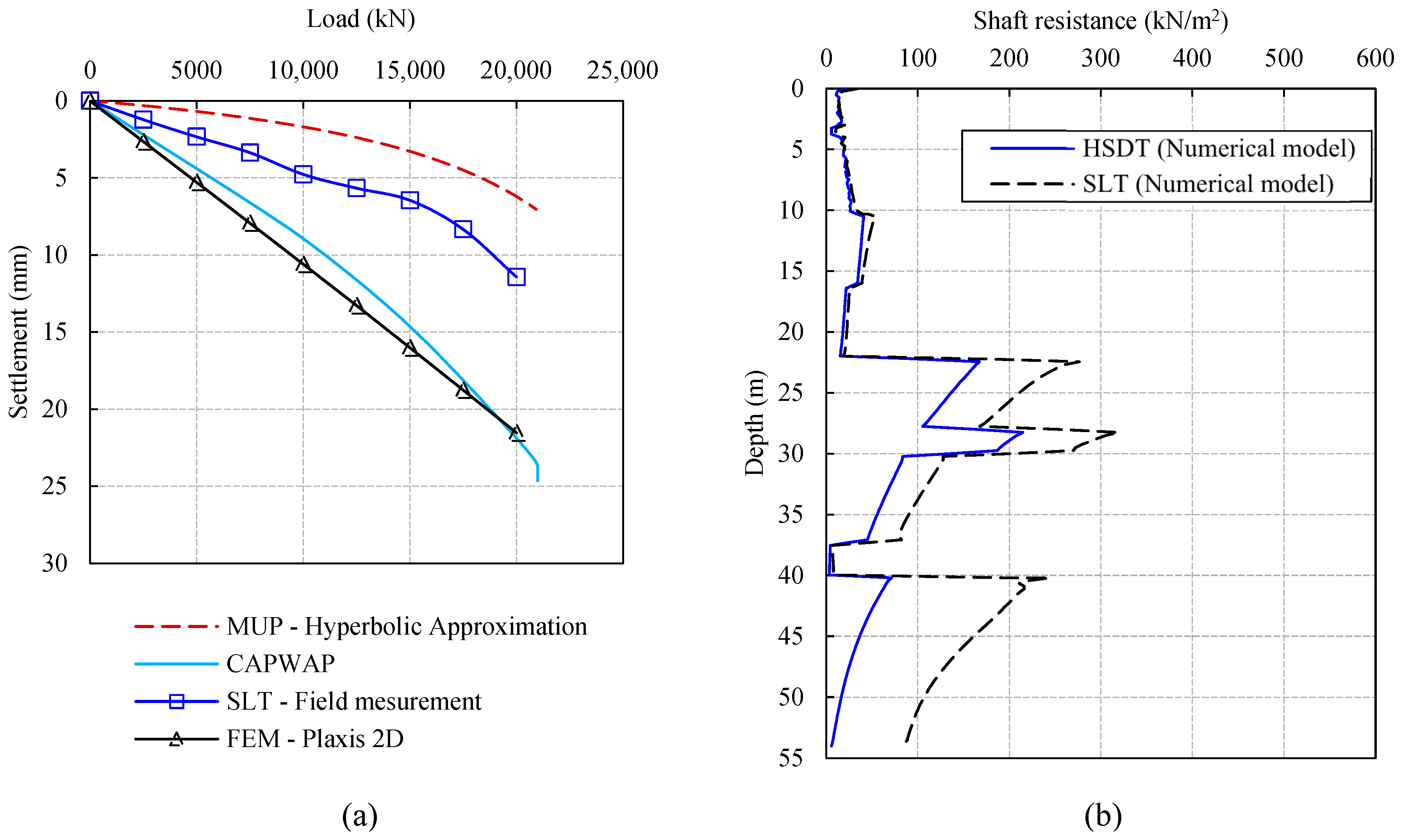
The soil resistance determined using the numerical modeling of the HSDT is the total compressive resistance, which includes both dynamic and static resistances. Additional analysis is required to separate the effects of dynamic soil-dependent behavior from the predicted total resistance, and subsequently, the mobilized static resistance is acquired, i.e., the calculated load-settlement response. The mobilized load-settlement curve is developed utilizing the MUP method discussed in the preceding section to separate all these effects. The comparison is performed between the predictions of the static numerical model (FEM), the MUP, and the CAPWAP (real HSDT) against the results of the real SLT. Figure 7a compares the static compressive load versus the settlement at the pile head for the real SLT, the FEM model, the CAPWAP, and the MUP hyperbolic approximation. The numerical analyses are performed using the deformation characteristics and shear strength parameters acquired from the specific signal-matching technique discussed in the previous section. The ultimate static resistance predicted through the CAPWAP is approximately 5% higher than the FEM model, and in both, the final displacement difference percentage is 11%. Although the CAPWAP calculations and the FEM model are in excellent correlation, the initial stiffness from the field SLT and the MUP prediction are quite high. It is noted that the varied loading rates [4] may be associated with the difference in the FEM and CAPWAP results compared to the field SLT. In addition, the deformation characteristics and shear strength parameters derived from the signal-matching analysis for both the FEM and CAPWAP may be slightly lower than the ground or soil investigation data.
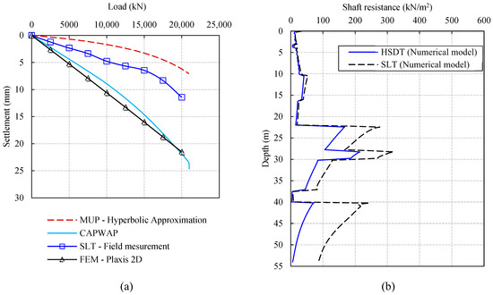
Figure 7.
(a) Comparison between measured field data, FEM modeling, the MUP method, and CAPWAP predictions. (b) Computed shaft resistance distribution along the pile (FEM).
In comparison to the field SLT results, the MUP method determines the mobilized static pile resistance and load-settlement response with relatively large differences. Nevertheless, the highest measured settlement during the SLT is 11.43 mm, whereas the computed value from the MUP method is 7.01 mm, with a difference of nearly 39%. At the unloading stage during the field SLT, the permanent settlement at the pile head is very small, 0.875 mm, which implies the total settlement is considered an elastic shortening of the pile. Table 2 compares the four methods in terms of the settlement, ultimate capacity, and resistance at the tip and shaft. Figure 7b further clarifies the mobilized shaft resistance from the HSDT numerical model versus the depth, with a substantial decrease compared to the skin friction distribution from the FEM modeling of the SLT. Also, it can be observed that the HSDT entirely mobilizes the skin friction of the upper layers, with a slight 5–15% lower than the SLT. In contrast to the higher layer, the skin friction of the lower layers is not fully mobilized, reducing approximately by 35–90% compared to the SLT. As a result of the improper free-falling drop-weight system selection, the transferred energy is insufficient to mobilize the pile fully at ultimate resistance.
Table 2.
Total resistance, shaft, and toe resistances from static and dynamic modeling (FEM) compared with field measurements.
The results derived from the non-linear numerical models agreed to some extent with the testing data recorded from the field full-scale loading tests performed on the bored piles. Consequently, the numerical simulations utilized during the analyses, comprising the free-falling drop-weight loading model, bored pile model, adopted and matched soil deposit properties, assigning viscous boundaries for dynamic calculations, and assumptions in Plaxis 2D, are verified.
8. Parametric Study
Numerical models are developed using the assumptions of the verified FEM model (i.e., the impact loading, boundary conditions, pile material, and adopted soil parameters) and then utilized to accomplish a comparative parametric analysis to understand the various aspects that affect the dynamic behavior of bored large-diameter piles during dynamic impact loading. In the parametric study, the variables considered are as follows: drop mass and height, cushion stiffness, surrounding soil type, and bored pile configuration.
The HSDT performed on bored piles of a different pile length to diameter ratio (L/D) installed in the same bearing layer (i.e., calcareous claystone fragments) is analyzed to explore the performance of the bored piles under impact loading. Moreover, the drop mass impact velocity applied to the pile top that affects the HSDT configuration’s ability to mobilize the pile’s static compressive resistance to its ultimate resistance is also investigated. The impulse force–time history induced by the HSDT on the head of the bored pile is mainly governed by the cushion stiffness and the drop weight; thus, these two variables are also explored. Using the MUP method, the acquired dynamic data are then interpreted.
8.1. Effect of Dropping Height
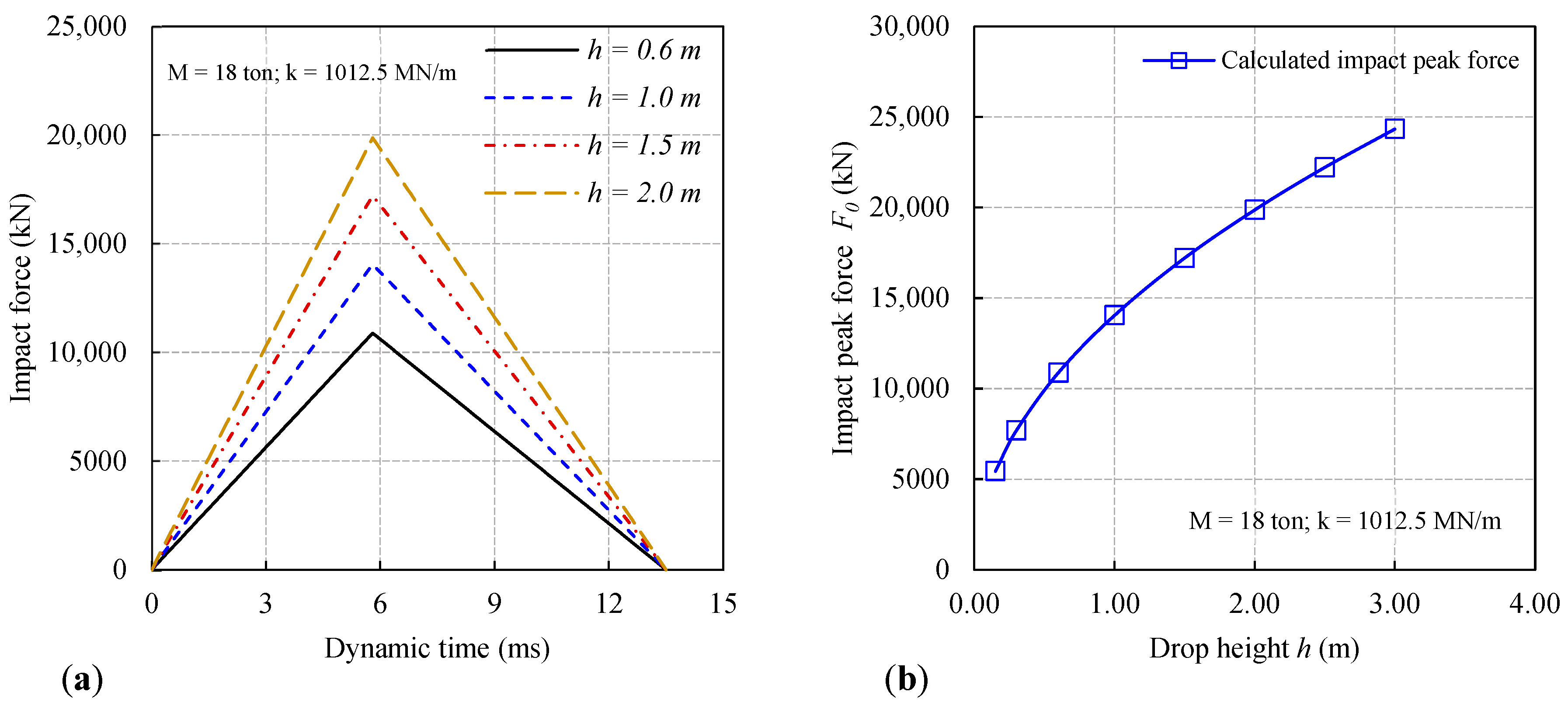
The bored pile responses to different mass-dropping heights (h) are studied. Only the impulse force–time response applied to the tested bored pile top is changed. Figure 8a indicates the impulse force–time response developed at different heights (h). The implemented force–time response for each dropping height (h) is produced in accordance with a triangular impulse load that is equivalent to the force developed utilizing the previous Equations (7)–(15). Four different mass-drop heights (h) are taken into account in this study. These dropping heights (h) are 0.6, 1.0, 1.5, and 2.0 m. It can be observed that when ξ < 1, the height of the dropping mass affects only the force amplitude, not its duration. Figure 8b depicts the calculated impact peak pile head force plotted against the drop height.
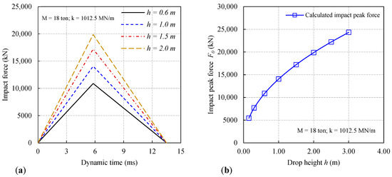
Figure 8.
(a) Shape of force pulses developed at different heights (h). (b) Influence of drop height on impact peak force.
The results demonstrate that the impact peak force increases with the increasing mass drop height. In addition, there is a consistent increase in the impact peak force and the drop height.
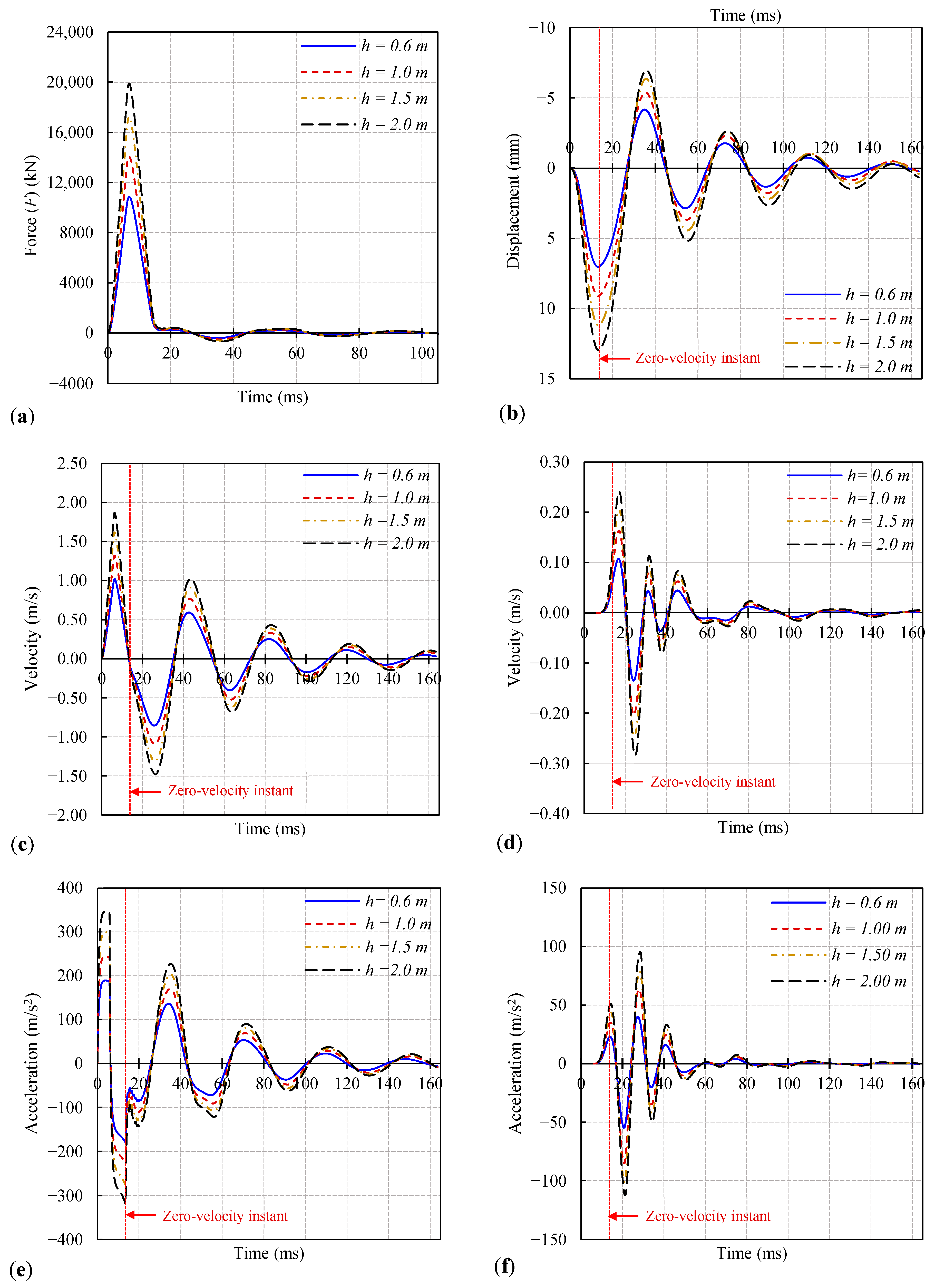
Figure 9 illustrates the computed pile dynamic responses in the HSDT at the top (force, displacement, acceleration, and velocity) and at the tip (acceleration and velocity) during the impact of different mass-falling heights. The acceleration and velocity responses at the top and tip of the bored pile are significantly different, demonstrating that the strain wave effect in the bored pile is strong due to the pile being longer. Furthermore, the pile dynamic response graphs are shown in Figure 9, indicating that as the mass-dropping height increases, the amplitude values of the displacement, impact force, acceleration, and velocity of the calculated pile portions also increase.
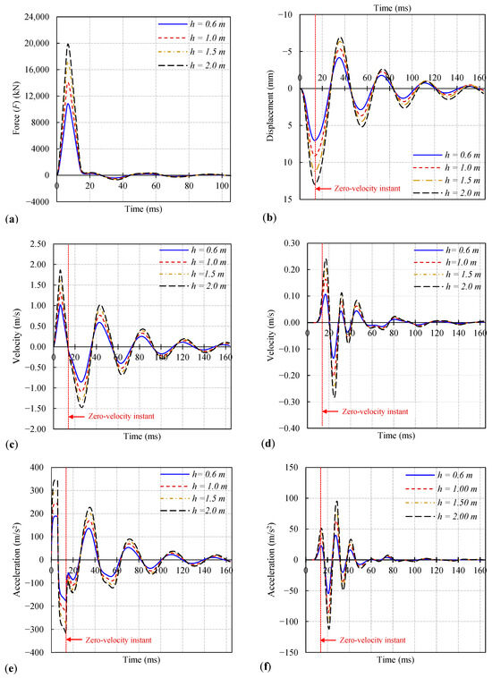
Figure 9.
Calculated pile responses in HSDT during the impact of different dropping heights ((a–c,e); impulse force, displacement, velocity, and acceleration at the top, respectively; (d,f); velocity and acceleration at the tip).
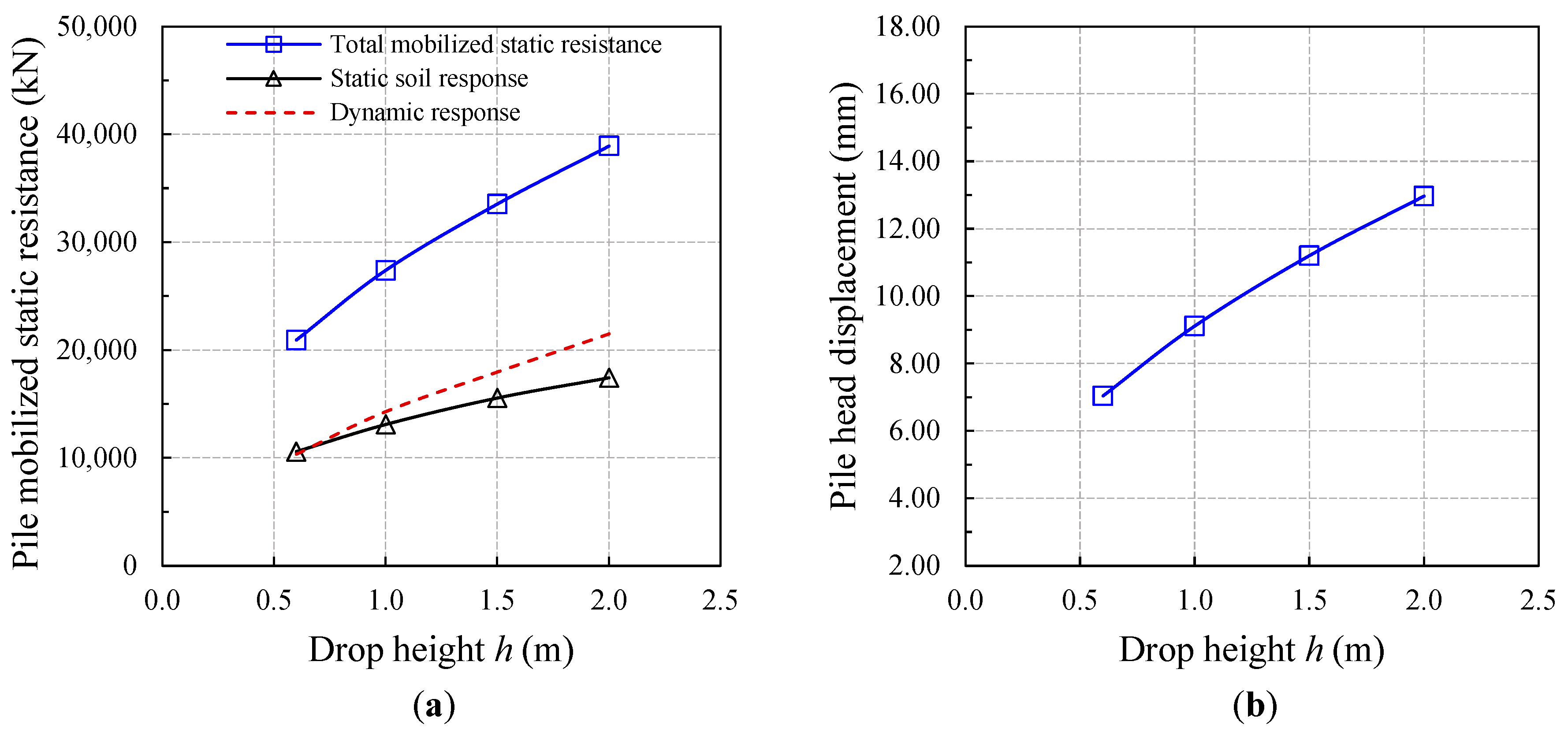
The derived static mobilized resistance through the MUP method at the unloading point (i.e., zero-instant velocity) can be estimated from the static soil response and the dynamic response (i.e., inertia force). Figure 10a shows the predicted mobilized static resistance of different drop heights. It can be observed that there is an almost linear correlation between the static response and the total mobilized resistance to the drop height. The dynamic response is defined as the difference between the total mobilized resistance and the static response. In addition, there is an apparent linear relationship between the drop height and the dynamic response. Figure 10b illustrates the calculated pile head displacements for each strike. The pile top displacement increases almost linearly as the mass-drop height (i.e., impact velocity) increases. This observation emphasizes the significance of employing adequate impact energy (i.e., dropping height) to move the pile top to a sufficient extent to mobilize its full resistance.

Figure 10.
(a) Influence of drop height on mobilized static resistance. (b) Calculated pile head displacement under different hammer-dropping heights.
8.2. Effect of Dropping Mass
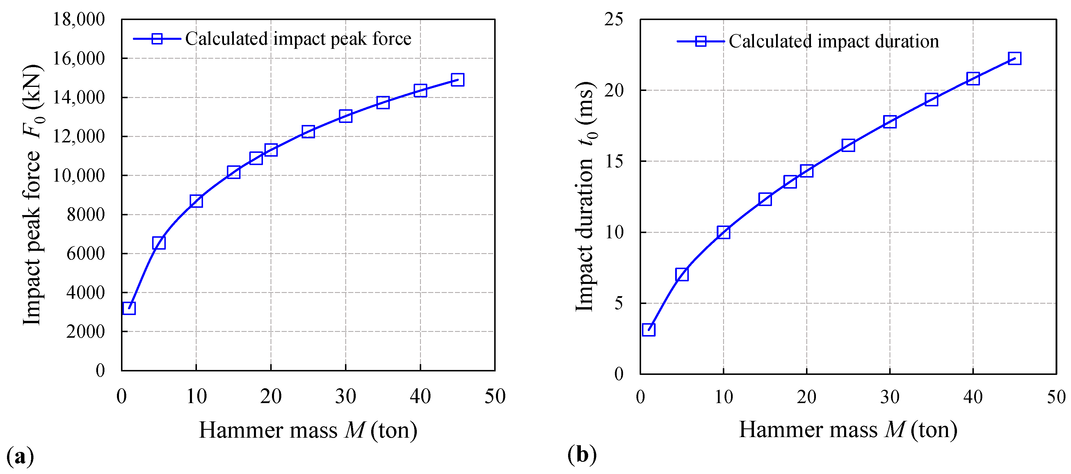
The dropping mass weight is adapted to displace the pile effectively to achieve the full mobilization of the pile resistance, which is a significant consideration when choosing a hammer cushion system. Using Equations (7)–(15), the applied force responses are calculated for each drop mass. Figure 11a,b demonstrate the drop-mass effect on the impulse peak force and impulse duration, respectively. The larger the drop mass is, the longer the impact duration and the higher the impact peak force.
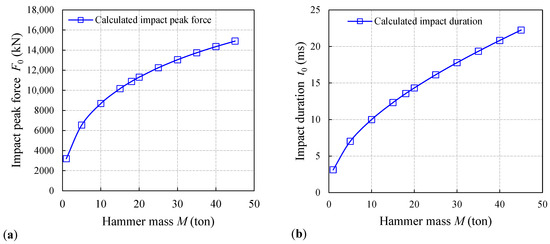
Figure 11.
Influence of drop mass on (a) impact peak force and (b) impact duration, respectively.
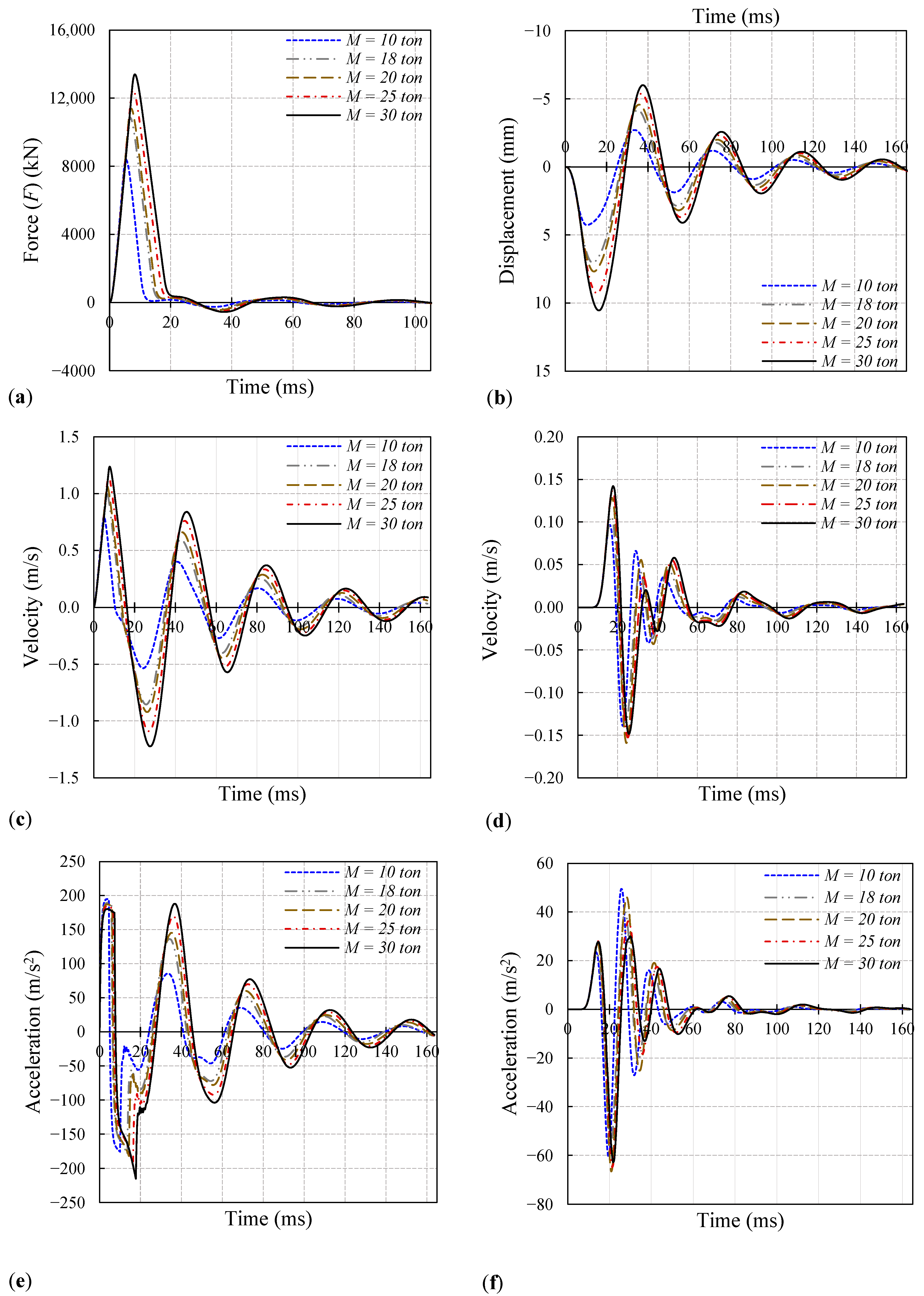
Five different values of drop mass, M = 10, 18, 20, 25, and 30 tons, are considered in the analysis. The mass-falling height (h) and cushion stiffness (k) are maintained for all cases at 0.60 m and 1012.5 MN/m, respectively. The calculated pile dynamic responses in the HSDT at the head (force, displacement, velocity, and acceleration) and at the tip (velocity and acceleration) under the impact of the hammer masses are shown in Figure 12. Moreover, the pile dynamic response plots demonstrate that as the hammer mass increases, the amplitude values of the displacement, impact force, acceleration, and velocity of the calculated pile sections increase as well. Also, there is a shift in the compression waves that propagate through the bored pile body due to the variation in the impact duration for each hammer mass.
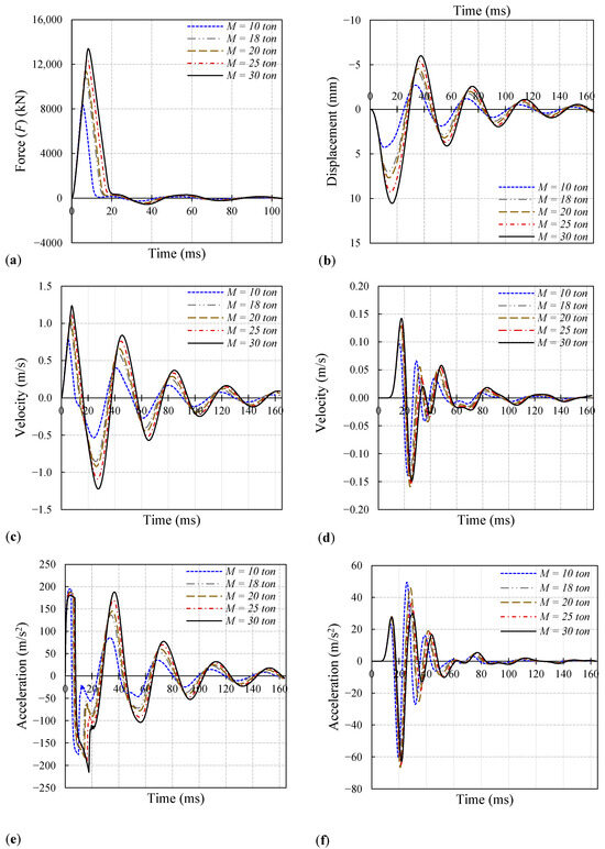
Figure 12.
Calculated pile responses in HSDT during the impact of different dropping masses ((a–c,e); impulse force, displacement, velocity, and acceleration at the top, respectively; (d,f); velocity and acceleration at the tip).
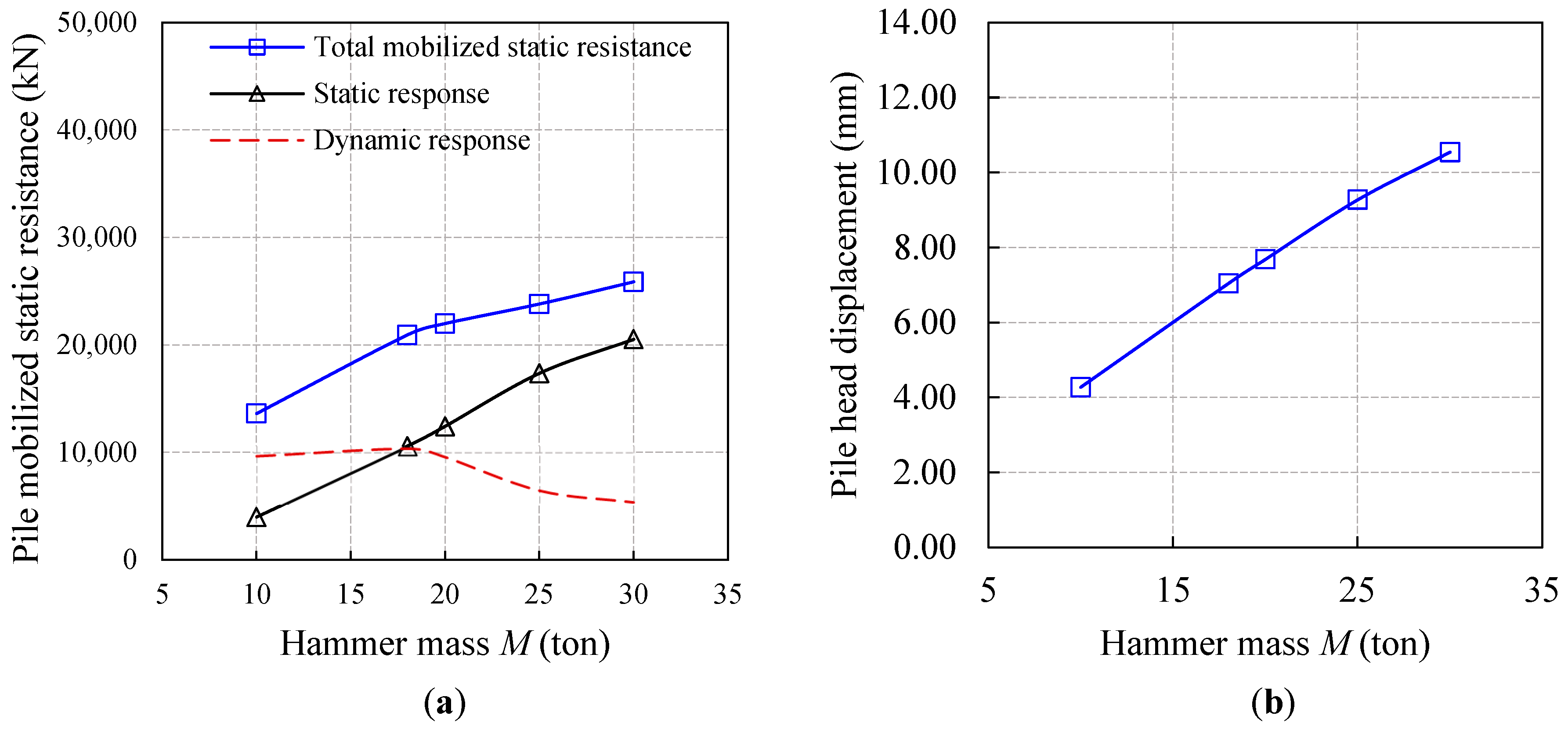
Figure 13a illustrates the derived mobilized static resistance for various hammer masses. There is an approximately linear relationship between the static response and the total mobilized resistance to the impact mass, as observed. In the beginning, as the drop mass (impact force) increases, the dynamic response increases almost proportionally linearly. After the drop mass reached a certain value (M = 18 tons), the dynamic response (i.e., inertia force) decreased disproportionately with the drop mass. The pile top displacement calculated for each mass below is presented in Figure 13b. The pile top displacement increases almost linearly as the drop mass (impact force) increases.
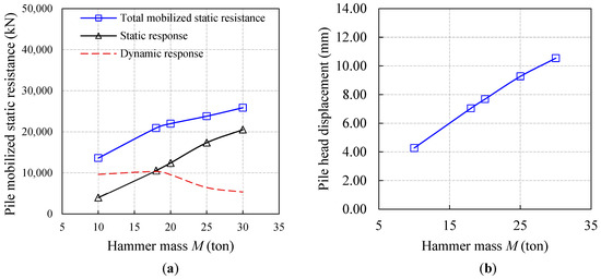
Figure 13.
(a) Influence of hammer mass on mobilized static resistance. (b) Calculated pile head displacement under different hammer mass.
A large drop mass is capable of maintaining the pile head force close to the impact peak force. Thus, a small drop mass will only develop a short impact event, which may not be sufficient to maintain a sustaining downward motion and pile skin and bearing resistance mobilization. As the impulse peak force is implemented to the bored pile top at the creation of the impulse event that mainly depends on the strike velocity, a higher dropping height will develop a higher impact peak force, similar to the effect of a larger drop mass.
Nonetheless, it is not possible to extend the impulse peak force, i.e., the duration of the impulse, by increasing the falling height. During striking, the destruction of the bored pile head is mainly the result of the higher impact force and an inefficient cushion. On the other side, a slowly dropping mass cannot develop sufficient force to mobilize the pile resistance. Hence, the most recommended impact force should fully mobilize the pile resistance without destroying the bored pile head. A longer impact duration is more effective for achieving deeper penetration, that is to say, the impact load should be developed by a larger drop mass with a lower falling height, not a smaller drop mass with a higher falling height.
8.3. Effect of Cushion Stiffness
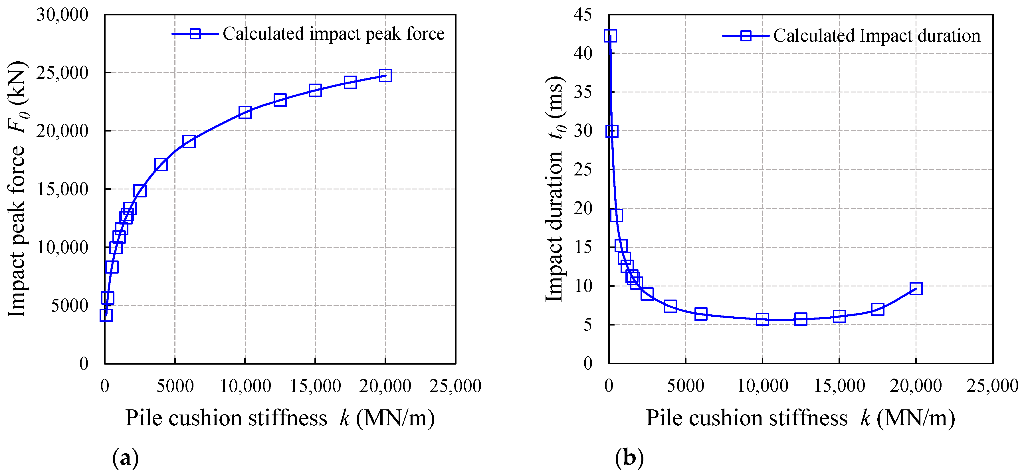
Pile cushions are required for cast-in-situ piles, for which they perform two functions. Firstly, they must minimize the possibility of stress concentration at the pile head. Secondly, they are developed to decrease the peak of striking stress at the pile head by extending the impulse forces out over time. Hence, the cushion stiffness, k, governs the impact force’s duration and amplitude at the pile top. Figure 14a,b demonstrate the cushion stiffness effect on the impulse peak force and impulse duration, respectively.
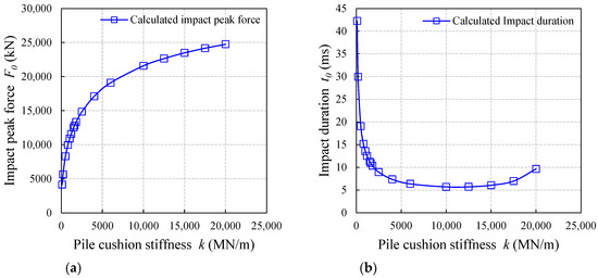
Figure 14.
Effect of pile cushion stiffness on (a) impact peak force and (b) impact duration, respectively.
As the pile pad becomes harder and harder, the impact duration decreases suddenly, and the impact peak force increases rapidly. After the cushion stiffness reaches a certain value (k = 10,000 MN/m), the impact duration gradually increases.
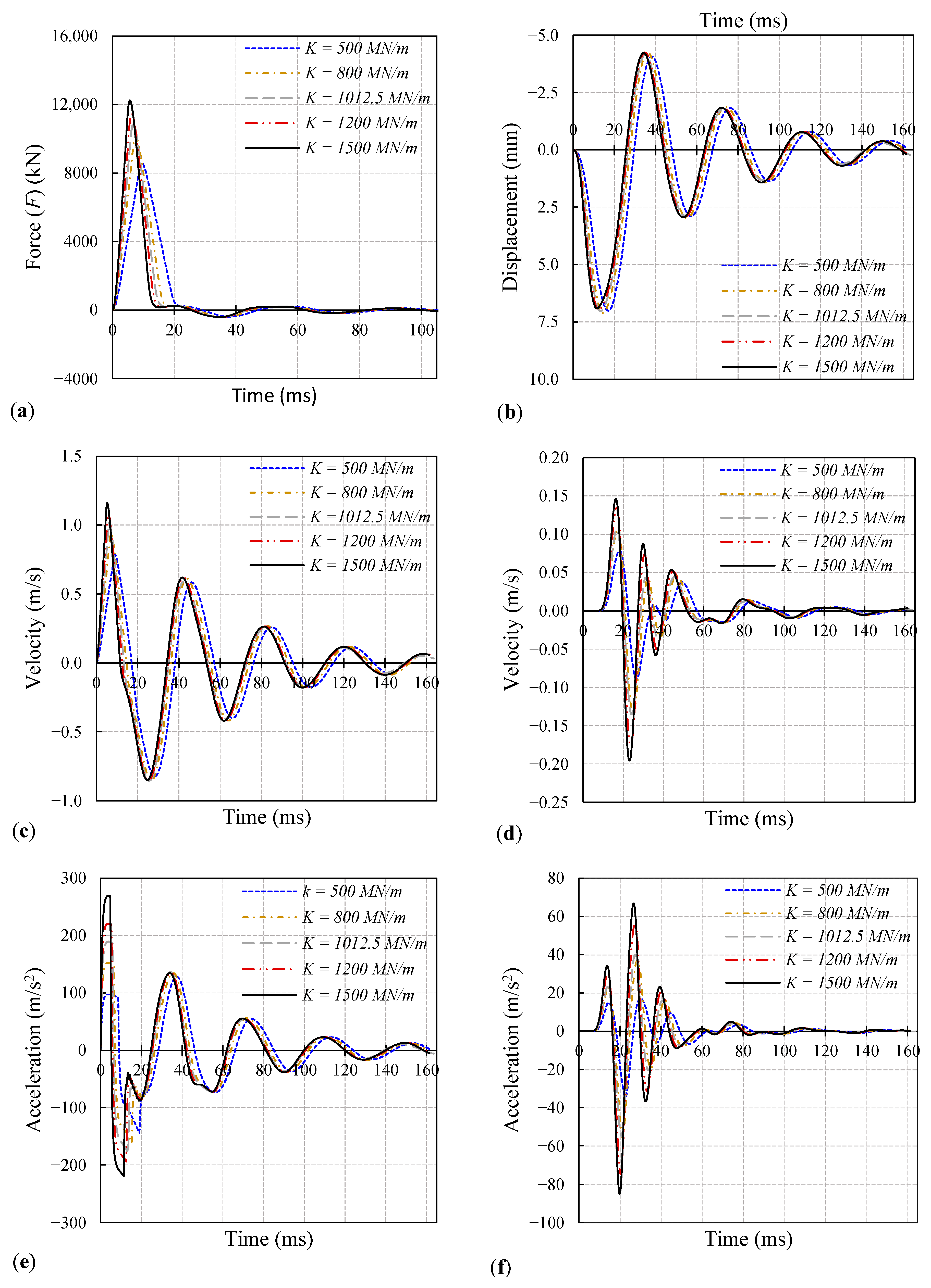
The following values of the cushion stiffness are considered in the analysis: k = 500, 800, 1012.5, 1200, and 1500 MN/m. These values are chosen to illustrate the overall stiff and soft hammer cushion systems. The drop mass and falling height are equal to 18 tons and 0.60 m, respectively. Figure 15 shows the predicted pile dynamic responses in the HSDT at the bored pile head (force, displacement, velocity, and acceleration) and at the bored pile toe (velocity, acceleration) under the impact of the drop mass, considering different cushion stiffness values. Also, the pile dynamic response graphs illustrate that as the cushion stiffness increases, the amplitude values of the impact force, acceleration, and velocity of the calculated pile sections increase as well. Due to the variation in the impact duration for each cushion stiffness, there is also a shift in the waves that propagate through the bored pile body.
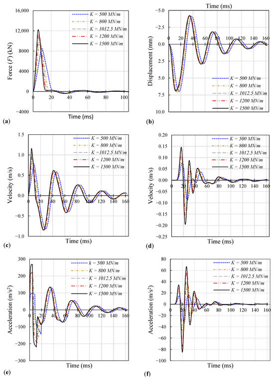
Figure 15.
Calculated pile responses in HSDT during the impact of different stiffness values of pile cushion ((a–c,e); impulse force, displacement, velocity, and acceleration at the top, respectively; (d,f); velocity and acceleration at the tip).
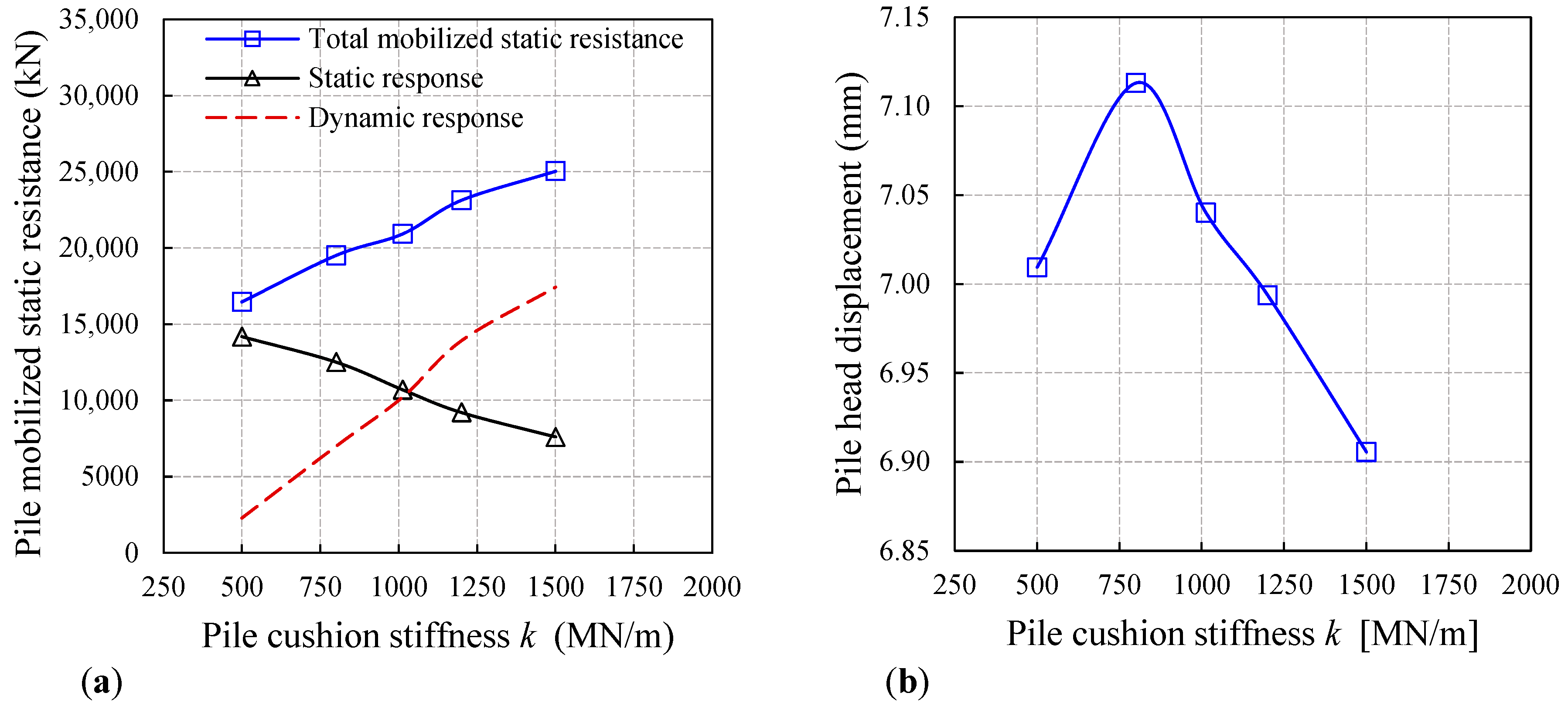
The predicted mobilized static resistances for different cushion stiffness values are shown in Figure 16a. As observed, there is an almost linear relationship between the total mobilized resistance and the dynamic response to the stiffness of the pile cushion. The static response decreased disproportionately with the increase in the pile cushion stiffness. Figure 16b represents the displacement of the pile top calculated for each cushion stiffness. Initially, as the cushion stiffness increases, the pile top displacement increases linearly. After the cushion stiffness reaches a specific value (800 MN/m), the displacement decreases almost linearly with increasing the cushion stiffness. There exists an optimal pile pad stiffness (approximately 800 MN/m, as shown in Figure 16b) for which the displacement (i.e., strain wave) will be significantly larger.
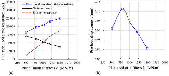
Figure 16.
(a) Effect of pile cushion stiffness on mobilized static resistance. (b) Calculated pile head displacement under different stiffness of pile cushion.
Too soft a pile cushion is unacceptable for a lower impact peak load and, as a result, lower penetration. Too stiff a pile cushion for a high peak impact force is also unacceptable due to the possibility of pile head damage. Adopting an appropriate pile cushion stiffness could optimize the striking efficiency.
8.4. Effect of Pile Length to Diameter Ratio (L/D)
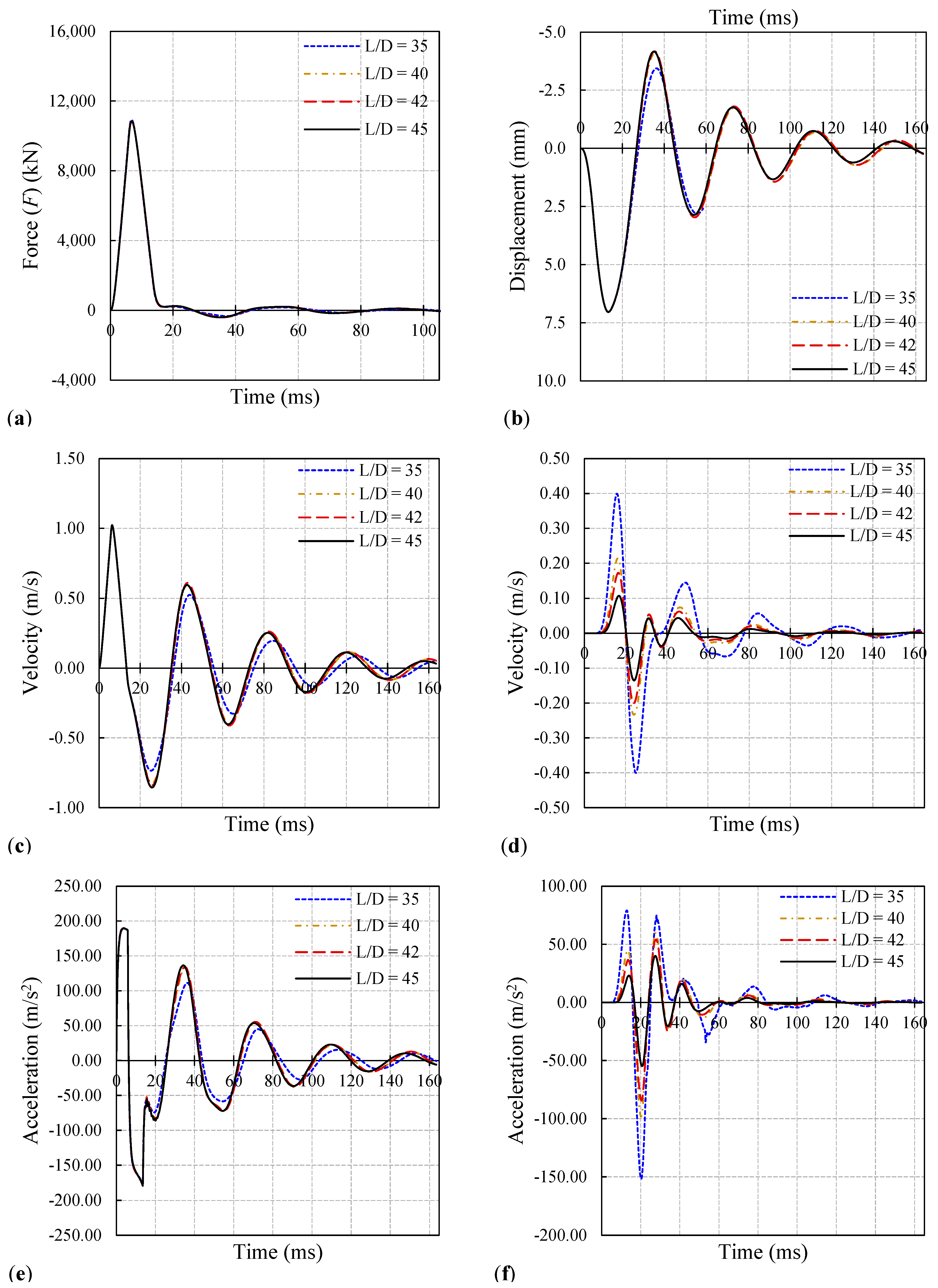
The HSDT performed on bored piles with different pile length to diameter ratios (L/D) installed in the same bearing strata (i.e., fragments of calcareous claystone) are analyzed to explore the performance of the bored piles under impact loading. In the analysis, the following pile dimensionless ratio (L/D) values are considered to be 35, 40, 42, and 45. The drop mass, falling height, and pile pad stiffness are kept at 18 tons, 0.60 m, and 1012.5 MN/m, respectively. Figure 17represents the calculated pile dynamic responses in the HSDT at the top (force, displacement, velocity, and acceleration) and at the tip (velocity, acceleration) under the impact of a drop mass for different values of the pile length to diameter ratio (L/D). For an of L/D 40, 42, and 45, the amplitudes (i.e., peaks) of the calculated impact force, displacement, acceleration, and velocity at the pile top are almost the same. In addition, the responses at the L/D = 35 case deviate from the responses of the other cases due to the significant variation in the embedded pile length in the bearing layer. Finally, as the L/D ratio decreases, the amplification values of the calculated responses (i.e., velocity and acceleration) at the pile base increase due to the effect of the stress wave phenomenon.
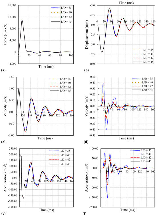
Figure 17.
Calculated pile responses in HSDT during the impact of different values of pile length to diameter ratio (L/D) ((a–c,e); impulse force, displacement, velocity, and acceleration at the top, respectively; (d,f); velocity and acceleration at the tip).
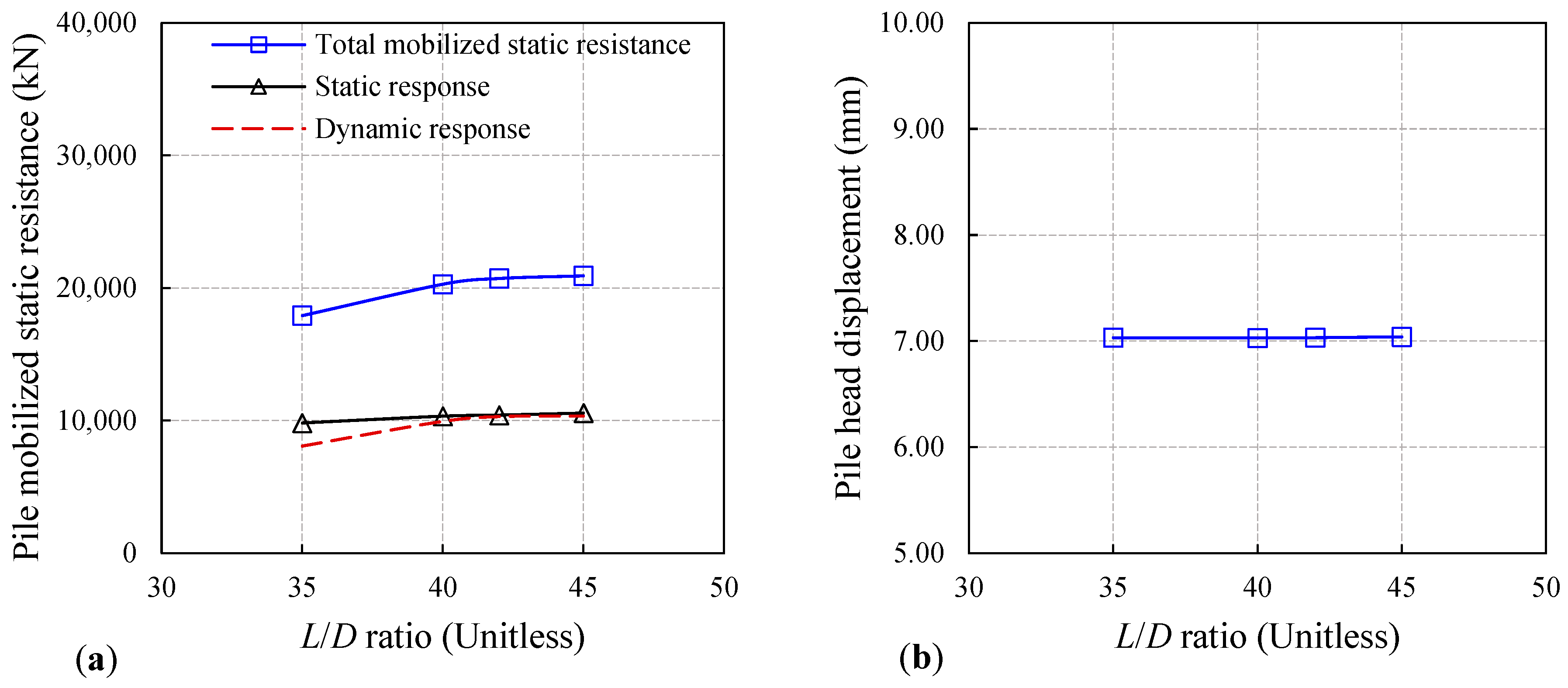
Figure 18a shows the derived mobilized static resistance for different L/D ratios. Initially, the total mobilized static resistance and the dynamic response increase nearly linearly as the L/D increases. After the L/D reaches a certain value (42), the total mobilized static resistance and the dynamic response increase slightly with the increasing L/D. The different cases of the L/D are exposed to the same energy (i.e., the hammer cushion system). Thus, the static response slightly changed due to the contribution of the skin friction and tip resistance in each case.

Figure 18.
(a) Influence of L/D ratio on mobilized static resistance. (b) Calculated pile head displacement for different values of L/D ratio.
As per the SLT, the pile skin friction is fully mobilized at first, and the tip resistance is gradually mobilized to its full capacity in the second stage. The dynamic response varied due to the inertia force contribution, which is calculated from the average of the acceleration at the tip and top of the bored pile. The computed pile head displacement for different L/D ratios is shown in Figure 18b. There is no effect on the calculated displacement due to the increase in the L/D ratio. This observation indicates that the upper layers surrounding the bored pile shaft are fully mobilized and subjected to the same applied energy.
9. Conclusions
Two-dimensional numerical models (FEM) are developed, utilizing Plaxis 2D software, to explore the non-linear behavior of bored piles through the HSDT and SLT. The model is validated using the results of an actual field test performed in New Alamein City. Two-dimensional axisymmetric FEM analysis is performed. The viscous boundaries are assigned and activated for dynamic calculations. The MC model is defined to characterize the non-linear response of the upper layers; in addition, the lower layer at the toe is modeled using the HS-small. The bored concrete pile is modeled utilizing the linear elastic material model regarding the non-porous drainage type with assigned concrete properties. The computed results agree to some extent with the measured testing data. The verified non-linear models are used to accomplish a comparative parametric analysis to understand the drop mass system characteristics that influence the dynamic behavior of bored large-diameter piles during dynamic impact loading. In the parametric study, the considered variables are as follows: drop mass and height, pile cushion stiffness, and bored pile length to diameter ratio (L/D).
Based on the findings of the verified model, parametric analysis, and the discussions in the preceding section, the conclusions made are as follows:
- (1)
- The FEM results matched well to some extent with the field records, proving that a 2D axisymmetric finite element model could accurately simulate both the SLT and HSDT, all based on the field test results of the case study on New Alamein City.
- (2)
- A geometry domain dimension of L (radius of the axisymmetric model) × 2L (depth of the model), where L is the length of the pile, is sufficient to model both the HSDT and SLT performed on bored piles without being affected by side boundaries, especially in the dynamic analysis.
- (3)
- It is proper to model the free-falling drop-weight system impact at the head of the bored pile using a triangular impulse load.
- (4)
- The justification of the soil parameters is the most significant advantage of the numerical model over the CAPWAP. So that the F and Zv signals can be matched, the results of the signal-matching analysis give values for deformation and shear strength characteristics that are either slightly lower or greater than the ground or soil investigation data.
- (5)
- The calculated load-displacement curves developed from analyzing the dynamic records (i.e., displacement, velocity, acceleration, and impact force responses) using the MUP method are consistent with the field results.
- (6)
- The most recommended impact peak force should be able to mobilize the soil resistance without destroying the bored pile head. A longer impact duration is more effective for achieving deeper wave penetration through the pile body. Thus, the impact load should be developed by a larger drop mass with a lower falling height, not a smaller drop mass with a higher falling height.
- (7)
- A larger drop mass reduces the dynamic response’s contribution (i.e., inertia force) and increases the static response in the total mobilized static compressive resistance. Hence, the recommended weight of the drop mass is at least 1% of the design compressive static resistance in very stiff soils (i.e., bored piles are established with a rock socket on bedrock), which is sufficient to maintain a sustained downward motion and mobilize enough skin friction and bearing resistance.
- (8)
- Too soft a pile cushion is unsuitable for a lower-impact peak force and, as a result, lower penetration. A pile cushion that is too stiff for a high peak impact force is also not suitable due to the possibility of causing pile head damage. The suggested optimal pile cushion stiffness equals 800 MN/m in this case, for which the high-strain wave will be significantly deeper.
- (9)
- The effect of the pile length to diameter ratio L/D is considered when adopting the dropping height and mass in the HSDT. Utilizing similar HSDT configurations on the bored piles with varied L/D ratios can lead to the same mobilized static resistance at higher L/D values, at which bored piles with larger L/D ratios required higher energy compared to piles with lower L/D ratios.
- (10)
- This study’s findings can be employed to develop guidelines and design procedures for the HSDT to be effectively performed on bored piles.
Author Contributions
Conceptualization, T.N.S. and R.H.; methodology, T.N.S. and A.S.E.-S.; software, A.S.E.-S.; validation, T.N.S., R.H. and A.S.E.-S.; formal analysis, A.S.E.-S.; investigation, A.S.E.-S.; resources, D.K.; data curation, K.K.; writing—original draft preparation, T.N.S., R.H. and A.S.E.-S.; writing—review and editing, T.N.S., D.K. and K.K.; visualization, D.K.; supervision, T.N.S. and R.H.; project administration, T.N.S. All authors have read and agreed to the published version of the manuscript.
Funding
This research received no external funding.
Data Availability Statement
The raw data supporting the conclusions of this article will be made available by the authors on request.
Conflicts of Interest
The authors declare no conflicts of interest.
References
- Wu, W.; Lu, C.; Chen, L.; Mei, G.; El, M.H. Horizontal Vibration Characteristics of Pile Groups in Unsaturated Soil Considering Coupled Pile—Pile Interaction. Ocean Eng. 2023, 281, 115000. [Google Scholar] [CrossRef]
- Wang, N.; Le, Y.; Tong, L.; Fang, T.; Zhu, B.; Hu, W. Vertical Dynamic Response of an End-Bearing Pile Considering the Nonlocal Effect of Saturated Soil. Comput. Geotech. 2020, 121, 103461. [Google Scholar] [CrossRef]
- Poulos, H.G. Pile Testing—From the Designer’s Viewpoint. In Proceedings of the 2nd Intrnational Statnamic Seminar, Tokyo, Japan, 28–30 October 1998; Kusakabe, O., Kuwabara, F., Matsumoto, T., Eds.; A. A. Balkema: Rotterdam, The Netherlands, 1998; pp. 3–21. [Google Scholar]
- Rizvi, S.M.F.; Wang, K.; Jalal, F.E. Evaluating the Response of Piles Subjected to Static and Multiple Dynamic Axial Loads. Structures 2022, 40, 187–201. [Google Scholar] [CrossRef]
- Salem, T.; Eraky, A.; Elmesallamy, A. Locating and Quantifying Necking in Piles through Numerical Simulation of PIT. Frat. Integrita Strutt. 2022, 16, 461–472. [Google Scholar] [CrossRef]
- Liu, X.; Wang, L.; Li, L.; Wu, W.; El, M.H.; Liu, H. Theoretical Model for Investigating Three-Dimensional Effect in Integrity Test of Open-End Pipe Piles. Ocean Eng. 2023, 286, 115526. [Google Scholar] [CrossRef]
- Tu, Y.; El Naggar, M.H.; Wang, K.; Rizvi, S.M.F.; Qiu, X. Dynamic Multi-Point Method for Evaluating the Pile Compressive Capacity. Soil Dyn. Earthq. Eng. 2022, 159, 107317. [Google Scholar] [CrossRef]
- Alwalan, M.F.; El Naggar, M.H. Analytical Models of Impact Force-Time Response Generated from High Strain Dynamic Load Test on Driven and Helical Piles. Comput. Geotech. 2020, 128, 103834. [Google Scholar] [CrossRef]
- ASTM D4945 Standard Test Method for High-Strain Dynamic Testing of Deep Foundations. Available online: https://www.astm.org/d4945-17.html (accessed on 3 May 2023).
- Hertlein, B.; Davis, A. Nondestructive Testing of Deep Foundations; John Wiley & Sons: Hoboken, NJ, USA, 2007; ISBN 0470034823. [Google Scholar]
- GRL Engineers, I. Case Pile Wave Analysis Program 1997. Available online: https://www.grlengineers.com/ (accessed on 11 April 2024).
- TNO Report TNO-DLT Dynamic Load Testing Signal Matching; The Netherlands Organization: The Hague, The Netherlands, 1996.
- Borgman, L.E.; Bartel, W.A.; Shields, D.R. SIMBAT Theoretical Manual (No.NCEL-TR-941); Naval Civil Engineering Laboratory: Port Hueneme, CA, USA, 1993. [Google Scholar]
- Pile Dynamics, I. CAPWAP Software. Available online: https://www.pile.com/products/capwap/ (accessed on 11 April 2024).
- Halder; Kumar, A. Pile Load Capacity Using Static and Dynamic Load Test. Master’s Thesis, Department of Civil Engineering, University of Engineering and Technology, Dhaka, Bangladesh, 2016. [Google Scholar]
- Goble, G.G.; Scanlan, R.H.; Tomko, J.J. Dynamic Studies on the Bearing Capacity of Piles. In Proceedings of the In Ohio Highway Engineering Conference Proceedings, Columbus, OH, USA, 2 May 1967. [Google Scholar]
- Long, J.; Hendrix, J.; Jaromin, D. Comparison of Five Differente Methods for Determining Pile Bearing Capacities; Wisconsin Highway Research Program: Madison, WI, USA, 2009.
- Holeyman, A.E. Keynote Lecture: Technology of Pile Dynamic Testing. In Proceedings of the Fourth International Conference on the Application of Stress-Wave Theory to Piles, The Hague, The Netherlands, 11 July 2022; pp. 195–215. [Google Scholar]
- Hussein, M.H.; Likins, G.E.; Hannigan, P.J. Pile Evaluation by Dynamic Testing during Restrike. In Proceedings of the Eleventh Southeast Asian Geotechnical Conference, Singapore, 4–8 May 1993; pp. 535–539. [Google Scholar]
- Likins, G.; Rausche, F. Correlation of Capwap With Static Load Tests. In Proceedings of the Seventh International Conference on the Application of Stresswave Theory to Piles 2004, Kuala Lumpur, Malaysia, 9–11 August 2004; pp. 381–386. [Google Scholar]
- Green, T.A.L.; Kightley, M.L. CAPWAP Testing—Theory and Application; IOS Press: Amsterdam, The Netherlands, 2005; pp. 2115–2118. [Google Scholar] [CrossRef]
- Vaidya, R. Introduction to High Strain Dynamic Pile Testing and Reliability Studies in Southern India. In Proceedings of the Indian Geotechnical Conference, Chennai, India, 14–16 December 2006; pp. 901–904. [Google Scholar]
- Rajagopal, C.; Solanki, C.H.; Tandel, Y.K. Comparison of Static and Dynamic Load Test of Pile. Electron. J. Geotech. Eng. 2012, 17, 1905–1914. [Google Scholar]
- Nath, B. A Continuum Method of Pile Driving Analysis: Comparison with the Wave Equation Method. Comput. Geotech. 1990, 10, 265–285. [Google Scholar] [CrossRef]
- Mabsout, M.E.; Tassoulas, J.L. A Finite Element Model for the Simulation of Pile Driving. Int. J. Numer. Methods Eng. 1994, 37, 257–278. [Google Scholar] [CrossRef]
- Feizee Masouleh, S. Evaluation of Design Parameters of Pile Using Dynamic Testing and Analyses. Ph.D. Thesis, Amir Kabir University of Technology, Tehran, Iran, 2008. [Google Scholar]
- Fakharian, K.; Feizee Masouleh, S.; Mohammadlou, A.S. Comparison of End-of-Drive and Restrike Signal Matching Analysis for a Real Case Using Continuum Numerical Modelling. Soils Found. 2014, 54, 155–167. [Google Scholar] [CrossRef]
- Bentley Systems, I. PLAXIS 2D Geotechnical Finite Element Analysis Software; Bentley Systems, Advancing Infrastructure: Delft, The Netherlands, 2022. [Google Scholar]
- Itasca Consulting Group, Inc. Fast Lagrangian Analysis of Continua FLAC 2D; Itasca Consulting Group, Inc.: Minneapolis, MN, USA, 2022. [Google Scholar]
- Naveen, B.; Parthasarathy, C.; Sitharam, T. Numerical Modeling of Pile Load Test. In Proceedings of the 4th China International Piling and Deep Foundations Summit, Shanghai, China, 26–28 March 2014; pp. 156–161. [Google Scholar]
- Liu, X.; Wu, W.; El, M.H.; Sun, J.; Tang, L. Computers and Geotechnics Theoretical Analysis of Dynamic Performance of Concrete-Filled Steel Tube Pile under Vertical Load. Comput. Geotech. 2024, 165, 105884. [Google Scholar] [CrossRef]
- Krasiński, A.; Wiszniewski, M. Static Load Test on Instrumented Pile—Field Data and Numerical Simulations. Stud. Geotech. Mech. 2017, 39, 17–25. [Google Scholar] [CrossRef]
- ASTM D1143 Standard Test Method for High-Strain Dynamic Testing of Deep Foundations. Available online: https://standards.globalspec.com/std/3828201/ASTMD1143/D1143M-07 (accessed on 17 June 2023).
- Krasiński, A. Numerical Simulation of Screw Displacement Pile Interaction with Non-Cohesive Soil. Arch. Civ. Mech. Eng. 2014, 14, 122–133. [Google Scholar] [CrossRef]
- Limas, V.V.; Rahardjo, P.P. Comparative Study of Large Diameter Bored Pile under Conventional Static Load Test and Bi-Directional Load Test. Malays. J. Civ. Eng. 2015, 27, 1–8. [Google Scholar]
- Keshavarz, A.; Malekzadeh, P.; Hosseini, A. Time Domain Dynamic Analysis of Floating Piles under Impact Loads. Int. J. Geomech. 2016, 17, 04016051. [Google Scholar] [CrossRef]
- Alwalan, M.F.; El Naggar, M.H. Finite Element Analysis of Helical Piles Subjected to Axial Impact Loading. Comput. Geotech. 2020, 123, 103597. [Google Scholar] [CrossRef]
- BSI ISO 22477-4:2018; Geotechnical Investigation and Testing—Testing of Geotechnical Structures—Part 4: Testing of Piles: Dynamic Load Testing. ISO: Geneva, Switzerland.
- Cao, W.; Chen, Y.; Wolfe, W.E. New Load Transfer Hyperbolic Model for Pile-Soil Interface and Negative Skin Friction on Single Piles Embedded in Soft Soils. Int. J. Geomech. 2014, 14, 92–100. [Google Scholar] [CrossRef]
- Han, G.-X.; Gong, Q.-M.; Zhou, S.-H. Soil Arching in a Piled Embankment under Dynamic Load. Int. J. Geomech. 2015, 15, 4014094. [Google Scholar] [CrossRef]
- Hölscher, P.; Barends, F.B.J. Statnamic Load Testing of Foundation Piles. In Proceedings of the Fourth International Conference on Application of Stress Wave Theory to Piles, The Hague, The Netherlands, 21–24 September 1992; Balkema: The Hague, The Netherlands, 1992; pp. 413–419. [Google Scholar]
- Maeda, Y.; Muroi, T.; Nakazono, A.; Inaba, N.; Takeuchi, H.; Yamamoto, Y.; Nakazono, N.; Takeuchi, H.; Yamamoto, Y. Applicability of Unloading-Point-Method and Signal Matching Analysis on the Statnamic Test for Cast-in-Place Pile. In Proceedings of the 2nd International Statnamic Seminar, Tokyo, Japan, 28–30 October 1998; pp. 99–108. [Google Scholar]
- Webb, D.L. Settlement of Structures on Deep Alluvial Sandy Sediments in Durban. In In-Situ Behavior of Soils and Rocks; British Geotechnical Society: London, UK, 1970; pp. 181–188. [Google Scholar]
- Begemann, H.K.S. General Report for Central and Western Europe. In Penetration Testing; National Swedish Building Research: Stockholm, Sweden, 1974; pp. 9–39. [Google Scholar]
- Papadopoulos, B.P. Settlements of Shallow Foundations on Cohesionless Soils. J. Geotech. Eng. 1992, 118, 377–393. [Google Scholar] [CrossRef]
- Bowles, J.E. Foundation Analysis and Design, 5th ed.; McGraw-Hill Inc.: New York, NY, USA, 1996; ISBN 0070067767. [Google Scholar]
- Plaxis 2D Material Models Manual; Bentley Systems, Inc.: Delft, The Netherlands, 2022.
- Dung, P.H. Modelling of Installation Effect of Driven Piles by Hypoplasticity. Master’s Thesis, Delft University of Technology, Delft, The Netherlands, 2009. [Google Scholar]
- Alpan, I. The Geotechnical Properties of Soils. Earth-Sci. Rev. 1970, 6, 5–49. [Google Scholar] [CrossRef]
- Hashash, Y.M.A.; Park, D. Non-Linear One-Dimensional Seismic Ground Motion Propagation in the Mississippi Embayment. Eng. Geol. 2001, 62, 185–206. [Google Scholar] [CrossRef]
- Bardet, J.P.; Ichii, K.; Lin, C.H. EERA: A Computer Program for Equivalent-Linear Earthquake Site Response Analyses of Layered Soil Deposits. University of Southern California: Los Angeles, CA, USA, 2000. [Google Scholar]
- Chen, R.P.; Wang, S.F.; Chen, Y.M. Study on Pile Drivability with One Dimensional Wave Propagation Theory. J. Zhejiang Univ. Sci. 2003, 4, 683–693. [Google Scholar] [CrossRef] [PubMed]
- Wang, F.; Wang, P.-F.; da Lyu, Z.; Zhao, Z.; Ma, B.-H. Dynamic Response of Super-Large-Diameter Steel Casing under Axial Impact Load. Ocean Eng. 2022, 244, 110249. [Google Scholar] [CrossRef]
- CH2M HILL, I. Geotechnical Report for the APE Yard Helical Pile Test Program; CH2M HILL, Inc.: Bellevue, DC, USA, 2013. [Google Scholar]
- Middendorp, P. Keynote Lecture: Statnamic the Engineering of Art. In Proceedings of the 6th International Conference on the Application of Stress Wave Theory to Piles, São Paulo, Brazil, 11–13 September 2000; pp. 551–562. [Google Scholar]
- Gunaratne, M. The Foundation Engineering Handbook; CRC Press: Boca Raton, FL, USA, 2013. [Google Scholar]
- Justason, M.D. Report of Load Testing at the Taipei Municipal Incinerator Expansion Project; Taipei City, Taipei, 1997.
- Middendorp, P.; Bermingham, P.; Kuiper, B. Statnamic Load Testing of Foundation Piles. In Proceedings of the 4th International Conference on Stress Waves, The Hague, The Netherlands, 21–24 September 1992. [Google Scholar]
- Alwalan, M.F. High Strain Dynamic Test on Helical Piles: Analytical and Numerical Investigations. Master’s Thesis, The University of Western Ontario, London, ON, Canada, 2019. [Google Scholar]
- Holscher, P.; Brassinga, H.; Brown, M.; Middendorp, P.; Profittlich, M.; Van Tol, F.A. Rapid Load Testing on Piles: Interpretation Guidelines; CRC Press: Boca Raton, FL, USA, 2011. [Google Scholar]
- Plaxis 2D Reference Manual; Bentley Systems, Inc.: Delft, The Netherlands, 2022.

Disclaimer/Publisher’s Note: The statements, opinions and data contained in all publications are solely those of the individual author(s) and contributor(s) and not of MDPI and/or the editor(s). MDPI and/or the editor(s) disclaim responsibility for any injury to people or property resulting from any ideas, methods, instructions or products referred to in the content. |
© 2024 by the authors. Licensee MDPI, Basel, Switzerland. This article is an open access article distributed under the terms and conditions of the Creative Commons Attribution (CC BY) license (https://creativecommons.org/licenses/by/4.0/).