Investigation of a Building with Male and Female Residents to Achieve Equality of Thermal Sensation Associated with Rational Use of Exergy and Energy

Abstract

The intensive use of air conditioning systems, primarily refrigerating, to promote thermal comfort in countries such as Brazil (a hot climate country) is changing the electrical energy consumption patterns and peak demand. Even with the increased number of appliances, we must learn to consume less energy to achieve similar outcomes with higher energy efficiency. Consequently, exergy analysis is used to evaluate the quality of these energy conversion systems. Four computational human thermal models were used to assess thermal comfort conditions: one man wearing lighter clothing, one man wearing traditional office clothing, and two women in the two types of clothing. We chose these four models since the body composition and basal metabolism rates for males and females differ. In addition, the insulation of clothes influences the temperature of the thermal environment, leading to a significantly lower percentage of people being unsatisfied, from 12.8% to values close to 5%. The outputs of these occupants are used as inputs for a computational model of the room to calculate its associated thermal loads and evaluate different temperature setpoints and their effects on thermal comfort and energy consumption. Results indicate that environmental temperatures above 24 $°$C and below 26 $°$C may lead to thermal comfort conditions, depending on the occupants’ clothing. Clothing would represent a thermal resistance of 0.7 CLO for men and women (when in the luteal phase of the menstrual cycle) and 0.8 CLO for women in the follicular phase when the environment is at 25 $°$C. Therefore, there is a significant reduction in the compression power of the central cooling system by about 2.2% compared to 24 $°$C and around 8% compared to ambient temperatures around 21 $°$C.

1. Introduction

Civilizations’ development and energy use are intrinsically connected [1]. From the energy return of investment index, all the technology created by society can relate to the transformation and conversion of matter and energy and the quality of energy conversion. Most significant technical and technological revolutions can be associated with these processes, from the beginning of man’s handling of fire to prepare food and keep themselves warm and far from danger (hunters and collectors) to crops and animal creation (farms and animal power usage) to the first industrial revolution. In this last one, steam produced mainly by coal burning empowered production and changed the dynamics of markets and society. However, while we are increasing energy conversion efficiency, there is a physical boundary. The Second Law of Thermodynamics governs any energy conversion between its different forms [2], and there are environmental impacts for all these technologies transforming energy sources into work. By acknowledging that it is highly relevant to humanity to aim for the rational use of energy and its quality, there have been several opportunities to evaluate exergy analysis in several societies, as shown in [3], and residential and commercial sectors are beginning to consider gender [4]. Just as primitive men used fire to keep themselves warm, modern society demands energy to promote thermal comfort. Buildings represent about 40% of global energy consumption and 30% of carbon emissions, most of which is associated with heating, ventilation, and air conditioning systems [5]. Therefore, there is a need to improve acclimatization systems for the more efficient use of energy. A way of evaluating the quality of energy usage is through exergy analysis.

1.1. Human Thermal Comfort and Exergy Analysis

Exergy analysis and its application to the human body is a tool that is already consolidated to evaluate thermal comfort conditions. Studies date from around three decades ago in three main groups, as indicated in references [6,7,8,9,10]. Nowadays, several investigations compare exergy analysis with thermal comfort conditions; for instance, differences due to muscle and fat mass composition [11] between males and females can be considered to obtain a more inclusive work environment [4]. Other authors have studied the relationship between CO₂ composition and human body exergy consumption [12], even through the application of CFD analyses to help assess the thermal environment [13]. Some review analyses compared the models in the literature, concluding that a unified exergy method is important to assessing thermal comfort conditions and the building environment using the same indicator [10,14,15]. The idea is that minimal points of destroyed exergy rate and exergy transfer to the environment represent thermal comfort conditions [10], and these thermodynamics figures are more sensitive to relative humidity and extreme conditions than the traditional predicted mean vote (PMV) and percentage of dissatisfied people with the actual thermal environment (PPD). Furthermore, minimizing the entropy generation and exergy destruction of the human body may contribute to a better life quality and lifespan [16].

1.2. Thermal Load Evaluation

This section details the Cooling Load Temperature Difference (CLTD) method for calculating thermal loads in environments. The article by Spitler et al. [17] provides a review of this method, proposed by the American Society of Heating, Refrigerating and Air-Conditioning Engineers (ASHRAE). According to Spitler et al. [17], this method for calculating thermal loads in environments was first proposed in the Cooling and Heating Load Calculation Manual [18], suggesting a means to estimate heat transfers between the environment and the surroundings, as well as heat generation within the environment (due to occupants and equipment). Cooling loads are calculated for each hour of the day, then they are added together to obtain the daily load or they are evaluated at the peak value. The procedures outlined by the CLTD method for calculating thermal loads are detailed for outdoor and indoor walls, ceilings, occupants, equipment, and glazing (or fenestrations), as depicted in Figure 1.

1.3. Objectives of This Article

Past work has aimed to combine minimizing exergy analysis and the building envelope [7], and the main concepts are summarized in [19]. Nevertheless, when there is a combination of males and females in the same thermal environment, the proposition of the best resistance (amount of clothes) to improve the thermal comfort index established by [10] has not yet been investigated in the literature. After the results of [4], some studies were found in the literature [20,21]. However, there is still little emphasis in scientific production on the exclusive analysis of the female body with all the indexes proposed. Moreover, we used an actual thermal environment in São Paulo, Brazil, to simulate occupational behaviors and differences.

Given that women represent more than 50% of the potential active workforce, the importance of promoting research focused on the female anatomy becomes evident, aiming for more significant equity in thermal sensation, bearing in mind that the following consequence is to reduce the building energy consumption. The main objective is to show that the occupants of the thermal environment need to change their clothes, increasing thermal resistance due to a barrier to air temperature. Furthermore, there must also be further investigation in order to achieve a higher number of satisfied people with lower energy demands.

2. Materials and Methods

This section details the parameters and values used in the methods presented in the introduction, along with the tools employed for solving the equations and developing the simulators.

2.1. Human Thermal Model

In order to obtain the temperature profiles used for the energy and the exergy analysis, Ferreira and Yanagihara [22] proposed a cylindrical model for the human body. The cylinder is the same height as the simulated body and comprises four layers. The innermost layer is the core, which encompasses bones, internal organs, and connective tissue. The core is followed by the muscle, fat, and skin layers, as shown in [4,11]. This simplification makes the model more flexible for varying body composition, allowing for the study of differences in the energetic and exergetic behavior between men and women. The volumes of each layer were calculated based on the percentage of body composition by mass and the specific mass, keeping the percentages of core and blood the same for men and women. The body compositions considered in the models are available in

Table 1. Mass percentage of each layer in the male and female models (based on [4,23]).

Layer	Male Model	Female Model
Core	39.73%	36.58%
Muscle	35.02%	29.28%
Fat	19.55%	28.44%
Skin	5.40%	5.40%
Blood	0.30%	0.30%

.

As the model simplifies the human body, it is impossible to maintain all parameters in the correct proportion. Once there is a definition of the height of the cylinders (the average height of an anatomy), the surface area of the skin layer will not correspond to the skin surface area of a human being with the same physical composition proposed by [24]. Similarly, if we preserve the surface area, the height no longer corresponds to reality. In this project, as in the literature [4,11], we decided to set the height of the cylinders, when necessary. As carried out by [25], we also normalized the energy and exergy parameters based on the surface area of the actual anatomy, since the energy transfer to the environment is the same.

Ferreira and Yanagihara [22] proposed a model based on a single anatomy of a male subject. The anatomies used were adapted from the primary source in [26]. The basal metabolism for each layer ${\dot{M}}_{bas}^{‴}$, density $\rho$, thermal conductivity k, and specific heat $c_p$ were recorded from [27,28,29,30,31,32,33,34,35]. Basal blood perfusion in cubic meters of blood per cubic meter of tissue w was constant, with consideration of the fact that the thermoregulation changes this initial value, as detailed in

Table 2. Density, basal metabolism, thermal conductivity, specific heat, and blood perfusion rate systematized as references previously cited and summarized in [4,11].

	$\mathit{\rho }$	${\dot{\mathit{M}}}_{\mathit{bas}}^{‴}$	k	${\mathit{c}}_{\mathit{p}}$	w
	(kg−3)	(W·m−3)	(W·m−1·K)	(kJ·kg−1·K)	$\times {\mathbf{10}}^{\mathbf{6}}$ (${\mathbf{m}}_{\mathit{bl}}^{\mathbf{3}}$·${\mathbf{m}}_{\mathit{ts}}^{-\mathbf{3}}$)
Core	1035	2629	0.5038	2.679	4157.5
Muscle	1006	684	0.5100	3.800	542.5
Fat	853	368	0.2100	2.300	76.7
Skin	1006	368	0.4700	3.680	361.7
Blood	1059	0	0.4700	3.850	-

. Also, all these thermophysical properties are the same for female and male models, e.g., one kilogram of muscle has the same characteristics in males and females. For all anatomies, standard weighted averages representative of the Brazilian population between 18 and 60 years [36] were considered: $1.71\mathrm{m}$ and $73.1\mathrm{kg}$ for males and $1.59\mathrm{m}$ and $62.5\mathrm{kg}$ for females [11]. Furthermore, the volume calculations were calculated using percentages of the total body mass.

As indicated by [37,38], most heat transfer between the blood and tissues occurs in the small arteries and veins. As in [4,11], the temperature profile across the tissues is constant, and the thermal exchanges between the layers are calculated through their thermal conductivity, taking into account the volume and shape of each layer. The energy balance for each tissue is given by Equation (1). Index i indicates the corresponding tissue/organ in this equation. Energy transfer to the environment may only occur in the core (via respiration) and skin (via convection, radiation, and evaporation).

$${\rho }_i{V}_i{c}_{p,i}\frac{d{T}_i}{dt}=-q_{i\to i+1}+q_{bl\to i}+V_i{\dot{M}}_i^{‴}-{\dot{E}}_{env}$$

(1)

Combining Equation (1) with Equation (2) using the model proposed by Pennes [37] and validated for the small vessels by [38], we obtained another energy balance. To solve these equations for each tissue (core, muscle, fat, and skin) and blood reservoir, we used the Engineering Equation Solver (EES©) to obtain the temperature profile directly when the steady state is achieved for all tissues within a chosen thermal environment.

$${\rho }_{bl}{V}_{bl}{c}_{p,bl}\frac{d{T}_{bl}}{dt}=\sum _{i=1}^4{q}_{bl\to i}$$

(2)

Equations (3) and (4) show the global energy and exergy balance. In these equations, M and $B_M$ are the energy and exergy metabolism [11], and ${\dot{E}}_{env}$ and ${\dot{B}}_{env}$ are the energy and exergy transfer to the environment, which occur through a combination of the effects of convection, radiation, sweat, and respiration. The term $\dot{W}$ is the performed power (usually disregarded in office environments), and ${\dot{B}}_d$ is the destroyed exergy rate. Its calculations are available in [4,11].

$$\frac{dU}{dt}=\dot{M}-\dot{W}-({\dot{Q}}_{conv}+{\dot{Q}}_{rad}+{\dot{H}}_e+\Delta {\dot{H}}_{resp})=\dot{M}-\dot{W}-{\dot{E}}_{env}$$

(3)

$$\frac{dB}{dt}={\dot{B}}_M-\dot{W}-({\dot{B}}_{conv}+{\dot{B}}_{rad}+{\dot{B}}_e+\Delta {\dot{B}}_{resp})={\dot{B}}_M-\dot{W}-{\dot{B}}_{env}$$

(4)

Past studies [4,11] conducted evaluations of different anatomies, where males and females showed different percentages of fat and muscle [23]. Moreover, females show a pattern of thermal behavior that is a function of the menstrual cycle, where the luteal (lower metabolism) and follicular (higher metabolism) phases show the most significant differences in metabolic behavior. Furthermore, we considered a difference in metabolism of 13.4% based on [39,40]. Another point that was evaluated is the difference in clothes, where men usually wear heavier clothes than women. The clothing varies from suits with a tie $I_{ml}=0.96\mathrm{CLO}$) to a skirt and social shirt ($I_{fem}=0.67\mathrm{CLO}$) [25].

Herein, we adopted typical office clothing for men and women. For the female computational models, the dress consisted of a bra, underwear, sheer socks, social shoes, a knee-length skirt, and a shirt with a long-sleeve, representing insulation $I_{cl{o}_{fem}}=$ 0.67 CLO. For the male computational model, a complete suit with tie was used, representing an insulation $I_{cl{o}_{ml,suit}}=$ 0.96 CLO [18]. In order to comparatively analyze the impact of clothing on thermal comfort conditions, a male model was also developed with lighter clothing, having the same clothing insulation as the female models ($I_{cl{o}_{ml,light}}=$ 0.67 CLO). Figure 2 shows a schematic representation of the presence of clothes in the model.

According to Fanger [25], the thermal activity index, $TAI$, shows the body’s energy balance and deviation to achieve thermal comfort conditions. Fanger [25] suggested a list of thermal sensations from very cold (−3) to very hot (+3), with 0 being comfortable. From a linear regression, it is possible to obtain the equation for the predicted mean vote ($PMV$) and an estimation of the percentage of people who are dissatisfied ($PPD$) with the thermal environment. Hence, it is possible to employ Equations (5) and (6) to assess $PMV$ and $PPD$, respectively.

$$PMV=\left[0.303exp\left(-0.036{\dot{M}}^{″}\right)+0.0028\right]TAI$$

(5)

$$PPD=100-95exp\left(-0.003353PM{V}^4+0.2179PM{V}^2\right)$$

(6)

2.2. Thermal Environment

The thermal environment modeled is based on the Philadelphia Building (Figure 3), a commercial building located in the district of Higienópolis, in the city and state of São Paulo. The building consists of 15 floors with commercial units, a bank branch on the ground floor, and a convention hall, whose division of main areas is shown in

Table 3. Division of the building envelope.

Environment	Private Area [m2]
Commercial unities	324
Bank branch	309
Convention room	122

. The Philadelphia building was chosen as the object of study because it was easy to obtain the parameters. The floor plans of the commercial units are standardized according to Figure 4. The ceiling height of each floor is 2.6 m. To simplify the modeling, the faces of the building were assumed as parallel to the cardinal directions (although this does not correspond to the reality of the building, such information would not significantly alter the result, but it would render the use of the tables in [18] almost impractical).

For the calculation of thermal loads associated with the walls and ceiling, the dimensions and parameters from

Table 4. Total wall area and correction factor for latitude for each face of the building.

Direction	Walls Area [m2]	LM
North face	25.28	−3.3
South face	25.28	1.6
East face	21.19	0
West face	42.41	0

were used. The areas were obtained from the floor plan in Figure 4 and the ceiling height. The adjustment factor $LM$ is tabulated and adjusts the data from the CLTD tables (whose standard is the Northern Hemisphere) for Southern latitudes (given the building’s location in the city of São Paulo). The month of December, typically a warm period in São Paulo, was chosen. The wall areas for each face have already excluded the window areas.

Other coefficients used for the modeling of walls and ceiling are given in

Table 5. Coefficients that were adopted for the walls and ceiling of the modeled building.

Coefficients	Value
Globa heat transfer coefficient of the walls ($U_{wall}$)	3.69 W·m−2·$°$C
Color factor for the surface of the wall ($K_{wall}$)	1
Global heat transfer of the roof ($U_{roof}$)	0.715 W·m−2·$°$C
Surface factor of color of the roof ($K_{roof}$)	1
Ceiling attic correction factor ($F_{roof}$)	0.875
Ceiling geographic correction factor ($L{M}_{roof}$)	0.5
Roof area ($A_{roof}$)	582.18 m2

. An adjustment factor for attics was considered for the ceiling due to the presence of inter-floor ceilings and ductwork. The construction of the ceiling was adopted as a 200 mm thick concrete layer. The color of the walls and ceiling was considered light, for which the color adjustment factor K is 1 [18].

For the calculation of the thermal load associated with glazing, the solar heat gain factors ($SHGF$) from

Table 6. Areas, correction factor ($LM$), and solar heat gain factor ($SHGF$) for the windows facing each direction.

Orientation	Windows Area [m2]	LM	SHGF
North	24.30	−3.3	136
South	39.16	1.6	154
East	50.54	0	669
West	29.95	0	669

were used, given as a function of São Paulo’s latitude and the orientation of the faces. The window shading coefficient ($S{C}_{window}$) considered was 0.81. The overall thermal exchange coefficient for windows ($U_{window}$) adopted was 3.69 W·m⁻² $°$C. The term $CLF$ is provided by the literature [18] and varies with the temperature throughout the day. The floors of the modeled building were considered to be of heavy construction in order to obtain the $CLF$.

The thermal load from equipment and lighting was calculated based on the area of the commercial units (multiplied by 15).

Table 7. Coefficients used in modeling the building’s equipment and lighting.

Coefficients	Adopted Value
Installed lamp power ($W_{lights}$)	5 W·m−2
Use factor ($F_{ul}$)	1
Application factor ($F_{sa}$)	1.2
Illumination of the unities ($A_{lights,unit}$)	324 m2
Equipment density ($W_{equip}$)	5.4 m2

shows the coefficients and parameters adopted in the model.

$$occupants=capability\times f_{occupants}$$

(7)

In order to represent the thermal load from occupants, the heat fluxes associated with the four models of the human body were used (i.e., the sum of the components of radiation, convection, sweat evaporation, and respiration for each individual). The maximum capacity was set as $capac=$ 730 people, and the occupancy factor $f_{ocup}$ was defined as a distribution with a peak concentration of people at 12 pm and 1 pm (hours with 100% occupancy), as shown in Figure 5. There is a substantial supposition here; people leave for lunch. Nevertheless, it was outside of the scope of this study to consider the thermal behavior of a person after going to lunch and changing their metabolic behavior (this approach will be employed in future analyses). To obtain the total number of occupants $ocup$, the relationship from Equation (7) was used. The distribution was made as 50% male and 50% female occupants. Among the women, 50% of them were set to be in the luteal phase and 50% in the follicular phase (since, according to [41], the menstrual cycle lasts an average of 28 days and the luteal phase lasts an average of 14 days).

2.3. Combination of the Models

This use of the models created to represent the occupants of the building implies a more responsive dynamic between the environment and equivalent thermal loads, as for each operative temperature, changes occur not only for the occupants’ thermal comfort indicators (such as $PMV$, $PPD$, and $B_d$) but also for the heat fluxes between the body and the environment.

For the exergy analysis of the modeled environment, the external environment was taken as the reference environment. In other words, in the expression of the exergy associated with thermal exchanges (walls, ceiling, glazing, lighting, and equipment) given by Equation (8), it was assumed that $T_0$ = $T_{ext}$. The surface temperature of thermal exchange was assumed to be the internal temperature of the conditioned environment, i.e., the operative temperature $T_{op}$.

$${\dot{B}}_{walls}={\dot{Q}}_{walls}\left(1-\frac{T_{ext}}{T_{op}}\right)$$

(8)

Following such logic, Figure 6 shows the exergy flow rates, where the external environment tends to decrease the exergy of the building, and the air conditioning system supplies exergy to the building in order to keep it at the operative temperature. To provide this exergy, it uses the compression power $W_{comp}$ obtained through the conversion of electrical energy.

The vapor compression refrigeration model proposed is shown in Figure 7, and it consists of the following: a compressor; a condenser, which exchanges heat with a cooling tower; a V_B expansion valve; a bypass valve called HotGas; and an evaporator, which allows thermal exchange between the refrigerant of the cycle and the water that cools the air. The function of the HotGas valve is to protect the condenser from over-pressure scenarios. Furthermore, an expansion valve, which is not shown in the figure but is also part of the circuit, is used to modulate the compressor power according to the momentary energy demand. The expansion valve is part of the compressor.

The fluid used in the simulations was the refrigerant R22 gas, the same used in the actual refrigeration system installed in the Philadelphia building, composed of two central chillers with a capacity of 100 TR each (i.e., about 351.7 kW each). Therefore, it is possible to draw parallels between the data obtained through simulations and the actual sizing of the equipment. The following assumptions were adopted:

• There is no pressure drop in the two condenser and evaporator flows, i.e., $P_{11}=P_{12}$, as well as $P_{13}=P_{14}$, $P_1=P_2=P_3$, and $P_4=P_5=P_6$;
• The cooling water pressure $P_{11}=P_{12}$, as well as the chiller cold water pressure $P_{13}=P_{14}$, are 20% higher than atmospheric pressure;
• The compressor is adiabatic and with isentropic efficiency $\eta$ = 0.75;
• Both the condenser and evaporator are adiabatic;
• The expansion valve is isenthalpic, i.e., $h_3$ = $h_4$;
• The fluid at the compressor outlet is superheated (at 5 $°$C above the saturation temperature).

2.4. Solving the System of Equations

Based on the theoretical fundamentals presented above, three large sections of equations were created, interconnected by a few key variables. In this way, the computational simulation code for the models was structured.

To solve these systems of equations, the EES© solver (Engineering Equation Solver) was chosen. This choice was mainly due to two reasons: first, for the practicality of solving implicit equations without the need to isolate variables as would be required in a C++ code, for example; and second, because EES© has an extensive library of properties and thermodynamic tables for various working fluids, allowing for the quick and automated consultation of the necessary values. In addition, EES© has the “Diagram Window”, a window where the input variables and main outputs can be highlighted and easily changed, similar to a simulator.

EES© uses a variant of Newton’s method for solving nonlinear algebraic systems, whose Jacobian matrix required for resolution is calculated numerically at each iteration. In order to enhance the efficiency of the calculation, sparse matrix techniques are applied to allow the solution of complex problems with up to 6000 variables in the standard version and 12,000 in the professional version.

The first computational section created was the thermodynamic model of the human body. The main inputs set to run a simulation are the ambient air temperature, relative humidity, and specific model parameters (clothing insulation, gender—that is, typical height and weight and body composition, menstrual cycle phase, and activity factor). After the iterative numerical solution, this first section provides the convergence output with apparent air temperature indicators ($PMV$ and $PPD$), exergy destruction rate ($B_D$), and heat fluxes (_ocup). These data will be inputs for the second section of equations. For greater efficiency in simulations, the four proposed models (women in the follicular phase, women in the luteal phase, men in full suits, and men in lighter clothing) were merged into a single program, whose variables are identified by the index.

The second computational section summarizes the model of the Philadelphia building. The main input data are the air temperature and relative humidity (translated by the same variable from the thermodynamic model of the human body), the thermal loads associated with the occupants, and their corresponding exergy destruction rates. After running the iterative numerical solution, this section of equations provides as outputs the exergy indicator $B_{D,edif}$ and the total thermal cooling load. By using the equation formulation in the “Equations Window” and inserting the main inputs in the “Diagram Window” of EES, it was possible to create a simulator that provides hourly thermal load curves associated with each element (ceiling, walls, windows, occupants, equipment, and lighting), thermal comfort indicators ($PMV$ average and $PPD$), and exergy destruction rate curves.

The third section consists of the equations associated with the vapor compression air conditioning refrigeration system. It also uses, in turn, the operative temperature and the total cooling thermal load of the building as input variables. Finally, it provides the exergy destruction rate in the refrigeration system $B_{D,ref}$ and the energy consumption. Similarly to the building block, the equations were entered in the “Equations Window” and the main inputs were placed in the “Diagram Window”.

3. Results

This section will validate the human body model and the application of the CLTD method. Moreover, the building’s energy consumption results are a function of the traditional and exergy-based indicators.

Validating the Human Body Thermal Model’s Behavior

Although the proposed model adopts simplifying assumptions that deviate from the actual geometry of the human body, after comparing the obtained results with experimental data explored in the literature, it is possible to validate its behavior for the purposes presented in this study. First, a review of the literature shows that other authors have simulated single-cylinder models. Ref. [25], one of the major references in the field of thermal comfort, initially proposed a model consisting of just one solid cylinder.

In order to create a scale of environmental temperature based on thermoregulation principles, ref. [42] created a two-node model to translate the thermal exchanges of a sedentary, naked occupant in a generic, uniformly heated and ventilated environment. As the author points out in his text, although there are more sophisticated proposals for representing the human body, simplified approaches still encompass important parameters, coefficients, and control systems to predict the quasi-equilibrium state of the individual with the environment. Additionally, they provide the three main parameters related to the assessment of thermal comfort: core temperature, temperature on the skin surface, and relative humidity on the skin surface. More complex models are more applicable in conditions other than sedentary and thermal neutrality, such as intense physical activity, localized thermal variations, and severe discomfort conditions, which do not apply to the thermal conditions simulated in this study. Furthermore, the proposed model closely resembles the one initially discussed by [43], whose validation was conducted by reproducing the same conditions adopted by [44] in their model and obtaining similar results.

The conditions adopted by [44] included a percentage of body fat of 17.6% and the energy metabolism per unit area (normalized by skin surface area) of 42.5 W·m⁻². By trial and error, ref. [43] found the air temperature that provided values close to the core and blood temperatures obtained by [44], in order to compare the parameters listed in

Table 8. Parameter values obtained by [44] compared with the ones obtained by the simplification of [43].

	Tikuisis et al. [44]	Ferreira and Yanagihara [43]
Body fat (%)	17.6 +/− 4.1	14.1
$M^{″}$ (W·m−2)	42.5 +/− 6.0	43.4
$T_{re}$ or Tn ($°$C)	37.52 +/− 0.29	37.5
$T_{\infty }$ ($°$C)	29.8	29.6
$T_s$ ($°$C)	37.32	37.4

. It can be seen that the values simulated in the model are considerably close and are fall within the uncertainty range of the data from [44], supporting the hypothesis that the models are compatible.

The enthalpic flow rates and heat exchanges with the environment were measured and simulated for an ambient temperature of 27.4 $°$C, as shown in

Table 9. Enthalpy flow rate associated with sweat and heat exchanges linked to radiation and convection. A comparison of publications results with the current model.

	Ref. [45] [W]	Ref. [43] [W]	Present Model [W]
Radiation	53.1	29.7	26.5
Convection	12.8	23.7	22.6
Diffusion and sweat	24.0	19.9	54.9
Total	89.9	73.3	104

. The model of a man dressed in lighter clothes was considered for the proposed model. It is noteworthy that although the heat associated with the vaporization of sweat is considerably higher than that proposed by [22,45], the heat associated with radiation and convection is of similar dimensions. Nevertheless, the former simulated naked models, with a neutrality temperature around 30 $°$C. It is clear that sweat mechanism is at low rates, whereas the anatomies and clothes studied here, at this temperature, are feeling “hot” based on ASHRAE scales.

Furthermore, for seated activity at rest, the models provided metabolic rates of ${\dot{M}}_{ml,sim}=$ 60.8 W·m⁻² for men in light clothing and ${\dot{M}}_{fm,fol,sim}=$ 54.8 W·m⁻² for women in the follicular phase. To validate the metabolic rates obtained, the metabolism equations proposed by [46] and the body surface area of [24] were consulted to obtain the metabolism per unit area ${\dot{M}}^{″}$. A weighting was also carried out according to the age group distribution statistics of the Brazilian population between 18 and 60 years old [36].

Metabolic rates of ${\dot{M}}_{ml,FAO}=$ 56.9 W·m⁻² were obtained for men and ${\dot{M}}_{fm,FAO}=50.4{\mathrm{W}·\mathrm{m}}^{-2}$ for women. It can be seen that the values obtained are computationally higher but still close to those found in the literature (note that the literature gives the basal or sedentary metabolism without the effect of a control system such as shivering). Moreover, in accordance with expectations, the male models showed higher metabolism than the female models in the follicular phase, and this was proportionally consistent (the FAO [46] proposes that the metabolism of men is 12.9% higher than that of women, and the metabolic increase in men obtained computationally was 11.0%). For the luteal phase, a metabolism of ${\dot{M}}_{fm,lut,sim}=$ 62.2 W·m⁻² was obtained.

The curves of thermal comfort indicators ($PMV$ and $PPD$) and exergy (${\dot{B}}_{env}$ and ${\dot{B}}_d$) as a function of air temperature $T_{air}$ for the four models were obtained by Molliet and Mady [4]. It was observed that, for all four models, the $PMV$ curve increases almost linearly with the rise in $T_{air}$, since this index represents the average assessment of the thermal environment, where (−3) indicates a very cold environment, and (+3) indicates a very hot environment. The $PPD$ curve resembles a parabola, with the minimum point coinciding with $PMV=0$ (i.e., in thermal neutrality, there is the minimum number of people dissatisfied with the apparent air temperature). As $T_{air}$ moves further away from neutrality, both to the left and to the right, $PPD$ increases, indicating more people in thermal discomfort. Regarding the exergy behavior, it is noteworthy that for low $T_{air}$, both the exergy destruction ${\dot{B}}_d$ and the exergy transfer rates to the environment ${\dot{B}}_{env}$ are high, and they decrease rapidly as $T_{air}$ approaches thermal neutrality, in agreement with the trend observed by [11]. At low temperatures, the thermoregulatory shivering mechanism increases body metabolism, while at temperatures higher than neutrality, metabolism tends to remain constant. Ribeiro and Mady [10] show that the $Q_{10}$ effect may be responsible for an increase in the destroyed exergy for high $T_{air}$ and $\varphi$. Nevertheless, these points are out of the scope of this manuscript, since these conditions do not occur under office conditions.

Garcia et al. [11] point out that only the minimum ${\dot{B}}_d$ is not sufficient to determine whether the body is in thermal comfort conditions, and it is necessary to assess whether ${\dot{B}}_{env}$ is also at an optimum point. This is because, for high temperatures and low relative humidities, ${\dot{B}}_d$ can be minimal, and the body may still experience thermal discomfort. However, given that such points are not in the typical ranges of temperature and relative humidity of air-conditioned environments ($40\%\le \varphi \le 60\%$ and 20 $°$C $\le T_{air}\le$ 30 $°$C), as they are typical of desert regions, the points of minimum ${\dot{B}}_d$ on the curves can be identified as points of thermal comfort. Finally, it is emphasized that the behavior of exergy transfer to the environment was unconventional, but tended to decrease, most likely due to some modifying mechanism added as a result of an additional thermal resistance, i.e., clothing. Comparing the curves related to the male model dressed in a complete suit and the female model in the follicular phase of reference [4], it can be observed that both the exergy destruction and the exergy transfer rates to the environment under comfort conditions are higher for the male model. Since men have a higher percentage of muscle mass and lower fat percentage compared to women, and given that muscles require more energy than fat, a higher metabolism is observed in men. The increase in metabolism implies more oxidation reactions and, consequently, more irreversibilities, causing higher exergy destruction and exergy transfer to the environment [4,11].

Another notable difference between the male and female models is the inflection point of the curves, i.e., the temperatures of thermal neutrality. The thermal comfort temperatures according to the [25] indicators ($T_{Fanger}$) and according to the exergy curves ($T_{exergy}$) for the male and female models in the follicular phase are shown in

Table 10. Thermal comfort temperatures obtained for male and female models in the follicular phase.

Model	${\mathit{T}}_{\mathit{Fanger}}$	${\mathit{T}}_{\mathit{exergy}}$
Man in full suit	23.5 $°$C	24.0 $°$C
Man in light clothes	25.0 $°$C	25.0 $°$C
Woman in the follicular phase	25.5 $°$C	26.0 $°$C

. It is noteworthy that both $T_{Fanger}$ and $T_{exergy}$ are lower for the model of the man wearing a full suit than for the woman in the follicular phase.

The hypothesis that differences in exergy behavior between men and women may be due to differences in clothing can be confronted by comparing the female model in the follicular phase with the male model wearing lighter clothing. When adopting the same clothing insulation for both models ($I_{clo}=$ 0.67 CLO), women still require higher temperatures $T_{Fanger}$ and $T_{exergy}$ to experience thermal comfort compared to men wearing lighter clothing.

Table 11. Thermal comfort temperatures obtained for female models in the follicular and luteal phases.

Model	${\mathit{T}}_{\mathit{Fanger}}$	${\mathit{T}}_{\mathit{exergy}}$
Woman in the follicular phase	25.5 $°$C	26.0 $°$C
Woman in luteal phase	24.8 $°$C	25.5 $°$C

shows the thermal comfort temperatures according to the [25] indicators ($T_{Fanger}$) and according to the exergy curves ($T_{exergy}$) for the female models in the luteal and follicular phases. It is possible to observe that, for the same relative humidity, during the luteal phase, women experience thermal comfort conditions at lower temperatures than during the follicular phase.

During the luteal phase, the increase in the concentration of both steroid hormones (estrogen and progesterone) in the blood has a notable influence on protein metabolism [47], inducing hyperinsulinemia and promoting the accumulation of glycogen in the pancreas [48]. This intensification of metabolic activity implies a higher rate of oxidation reactions, generating more irreversibilities and consequently higher values of ${\dot{B}}_d$ and ${\dot{B}}_{env}$. During the luteal phase, there is also an increase in fat deposition in adipose tissue, promoting catabolic effects on protein metabolism [48]. It is possible to observe from [4] that during the luteal phase, the exergy values in the comfort range are really higher than during the follicular phase. This result can also be associated with the decrease in skin thermal conductance [49]. With lower thermal conductance, women’s bodies require lower ambient temperatures to maintain thermal neutrality, since heat exchange with the environment is hindered. A comparative analysis of the male model wearing a full suit and dressed in lighter clothes shows that thermal comfort conditions are reached at different temperatures, with lighter clothes having a higher temperature (Table 10). Wearing thicker clothing hinders the transfer of heat produced by metabolism to the environment, given the thermal insulation of the clothing. Therefore, in order for the body to reach the temperature profile of thermal neutrality, the ambient temperature must be lower. Moreover, the behavior of the exergy transfer curve to the environment (${\dot{B}}_{env}$) was different from that obtained by [11] for the naked model, since for temperatures above the minimum exergy destruction rate (${\dot{B}}_d$), it tends to decrease rather than increase. This effect is most likely attributed to the presence of additional thermal resistance imposed by the clothing.

Figure 8 displays the hourly curves of the thermal loads associated with the roof, walls, glazing, lighting, equipment, and occupants in the building model. This first simulation was obtained by setting the internal temperature to 24 $°$C. It can be observed that the highest thermal load is associated with the glazing, as the Philadelphia building has a highly glazed architectural facade, which cancels out the intended effect of using bricks (insulating material). The peak thermal load occurs around 5 pm, mainly due to the thermal inertia of the building elements. In addition, the thermal load from glazing is highest during the illuminated period of the day, due to the incidence of solar radiation. Glazing works act as a greenhouse, being highly transparent to solar radiation and opaque to thermal radiation emitted by occupants, lighting, and equipment, thus retaining energy inside the building.

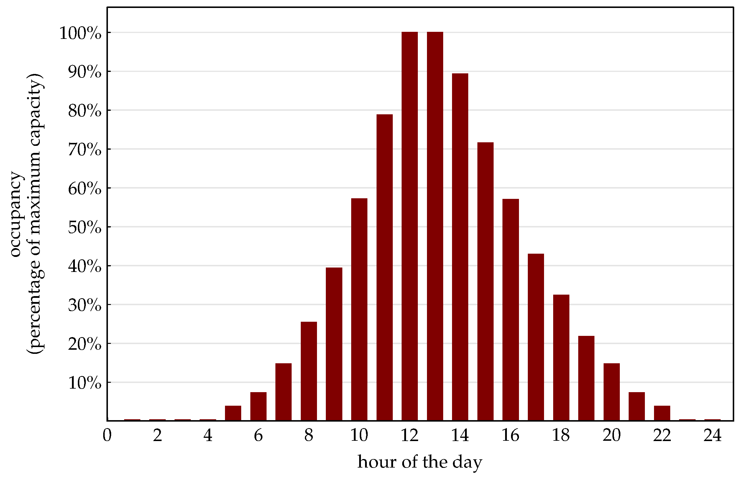
Since the order of magnitude of the thermal load associated with glazing is greater than that of the others, in order to facilitate the visualization of the behavior of the thermal load curves associated with occupants, lighting, equipment, walls, and ceiling, the corresponding region in the graph in Figure 8 was zoomed in, thus generating Figure 9. It can be observed that the second highest thermal load is associated with the building occupants. The peak occurs between 12 pm and 1 pm, the period of maximum occupancy (bearing in mind that there is a hypothesis of the occupant not leaving the room to avoid additional refinements regarding exercise to go lunch and other aspects), and it is approximately 78 kW. The thermal load curves associated with lights and equipment have a similar behavior, being nearly constant and present only during business hours (i.e., when they are in use). The thermal load curves associated with walls and ceilings have a similar sinusoidal profile, since they are made up of the same mechanisms (conduction, radiation, and convection on the surfaces). It is worth highlighting the “delay” in the peak thermal load caused by the bricks (6 pm) and, therefore, the need to pay attention to such aspects when designing the building. In a tropical country like Brazil and a commercial city such as São Paulo, there must be a balance between the benefits of glazing and the problems with thermal load, mainly in extreme scenarios, as those which occurred in 2023.

In order to assess the thermal comfort of the occupants, simulations were carried out for operative temperatures of 20 $°$C, 22 $°$C, 24 $°$C, and 26 $°$C. The data obtained have been transferred to

Table 12. Building thermal load (${\dot{Q}}_{total}$), exergy destruction rate (${\dot{B}}_d$), estimated average vote ($PMV$), and percentage of dissatisfied people ($PPD$) obtained for the building simulation for operating temperatures of 21, 22, 23, 23.5, 24, 25, 25.5, and 26 $°$C.

${\mathit{T}}_{\mathit{o}}$ [$°$C]	21	22	23	23.5	24	25	25.5	26
${\dot{Q}}_{total}$ [kW]	638	624	612	605	599	586	580	574
${\dot{B}}_d$ [kW]	587	575	563	557	551	540	534	529
$PMV$ [−]	−0.46	−0.34	−0.20	−0.11	−0.01	0.22	0.34	0.48
$PPD$ [%]	9.5	7.6	6.1	5.6	5.5	6.8	8.4	10.8

. Regarding the thermal comfort of the occupants at a temperature of 21 $°$C, the PPD (predicted percentage of dissatisfied) indicates that 9.50% of all occupants are in thermal discomfort. At the optimum comfort point (minimum PPD), 5% of the occupants experience thermal discomfort. Additionally, the PMV (predicted mean vote) indicates that the majority of occupants rate the environment as cold (PMV < 0). It is possible to observe that the PMV curve undergoes an inflection between the operative temperatures of 24 $°$C and 25 $°$C, as it changes from negative values to positive values. This indicates that the optimum temperature point, where the PMV is closest to 0 and the PPD approaches its minimum point (5%), lies between such temperatures.

By analyzing Table 12, it is possible to note that the thermal load of the building decreases with the increase in the temperature setpoint of the air-conditioned environment. The exergy destruction rate, however, also tends to decrease with the increase in the operative temperature, but a curve inflection is observed between temperatures of 25.5 $°$C and 26 $°$C, which suggests a minimum point. In terms of thermal comfort indicators ($PMV$ and $PPD$), there is clearly an optimum point between temperatures of 24 $°$C and 25 $°$C, indicated by the PPD approaching the minimum of 5% and the PMV reaching zero. However, it is worth noting that the exergy destruction rate reported in Table 12 pertains to the entire building and not just the occupants. Therefore, it does not serve as an indicator of thermal comfort (unlike the exergy destruction rate discussed in Table 10). This indicator is a way of evaluating the use of resources and the optimization of the system, seeking to minimize it.

The graph in Figure 10 was constructed by combining the data obtained from the human body simulations and the thermal loads from Table 12. It shows the thermal comfort points for the four human body models (according to the exergy criteria and according to the criteria by [25]), as well as the thermal load curve to be removed from the building for the operative temperature range of 23.5 $°$C to 26 $°$C. It is possible to observe a linear reduction in thermal load as the operative temperature of the air conditioning system increases.

By examining Figure 10, it is also noticeable that, under both approaches, the male model wearing a full suit (represented by HT) experiences thermal comfort at lower temperatures than the other models, and women in the follicular phase (MF) require higher temperatures to be in thermal comfort. The female models in the luteal phase (ML) and the male model wearing lighter clothes (HL) showed similar thermal comfort conditions, with their tendency more closely resembling that of the female model in the follicular phase (MF), experiencing thermal comfort at higher temperatures. This may be associated with increased metabolic activity during the luteal phase, which is even higher than that of men.

By comparing the comfort points and the thermal load line, it can be observed that adopting temperatures close to the comfort conditions of the male models with light clothing (HL) and women in the luteal phase (ML), around 25.5 $°$C (580.10 kW), would represent a 4.1% lower thermal load at the peak compared to the temperature for the male model wearing a full suit (HT), at approximately 23.5 $°$C (604.89 kW). On an operational day, approximately 585 Wh is saved with artificial air conditioning.

Ref. [50] establishes that the recommended dry bulb temperature range for indoor operation should be from 23 $°$C to 26 $°$C in the summer and from 20 $°$C to 22 $°$C in the winter. Therefore, since energy consumption decreases linearly with operating temperature, reducing this operating temperature range of air conditioning equipment to 24.5 $°$C to 26 $°$C would not only provide greater comfort to occupants but also reduce the cooling thermal load and, consequently, offer economic advantages.

Fisk et al. [51] estimates that improving thermal environments in offices in the United States would result in a productivity increase of up to 5%, which represents gains of up to 125 billion dollars annually. Ref. [52] conducted an analysis of the relationship between work performance and ambient temperature, and the results indicated a drop in human productivity of 2% for every 1 $°$C increase in temperature, only within the range of 25 $°$C to 32 $°$C. No significant change in performance was observed for the range between 21 $°$C and 25 $°$C. However, the operative temperature alone is not sufficient to assess productivity, since human performance is more associated with the perception of temperature, in terms of thermal comfort [53]. Lan et al. [54] also points out that environments whose $PMV$ is excessively high or low (far from neutral) lead to a reduction in human performance.

McCartney and Humphreys [53] point out that for non-repetitive activities, such as those in most offices, it is challenging to define methodologies for measuring productivity without using subjective and/or biased criteria. However, even though it is not possible to accurately assess the degree of increased productivity, it was observed that productivity did vary according to the occupants’ perception of temperature. Thus, the literature strongly suggests a link between promoting thermal comfort and productivity, even though establishing these relationships directly and measurably requires a more thorough investigation. In light of this, conducting thermal comfort studies for the adaptation of work environments can not only lead to economic advantages associated with energy savings but also to higher work performance from employees [55].

Thus, it is possible to propose better operating conditions to save energy and provide comfort to more occupants. One way to achieve such an effect more efficiently is to propose changes in clothing habits in conjunction with an increase in the operating temperature of the air conditioning system. By evaluating the same parameters for the human body and the building, but considering that instead of wearing a suit, men are wearing lighter clothes, we have the data in

Table 13. Building thermal load (${\dot{Q}}_{total}$), exergy destruction rate (${\dot{B}}_d$), estimated average vote (PMV), and percentage of dissatisfied people (PPD) obtained for the building simulation for operating temperatures of 21, 22, 23, 23.5, 24, 25, 25.5, and 26 $°$C, considering that men are wearing lighter clothes.

T [$°$C]	21	22	23	24	25	25.5	26
${\dot{Q}}_{total}$ [kW]	639	626	613	599	586	580	574
${\dot{B}}_d$ [kW]	588	576	566	536	540	534	529
$PMV$ [−]	−0.60	−0.49	−0.36	−0.21	0.003	0.14	0.28
$PPD$ [%]	12.8	10.2	7.8	5.9	5.0	5.4	6.7

.

From Table 13, it can be observed that, at 25 $°$C, only 5.01% of the occupants would be dissatisfied with the thermal environment. Now, by fixing the temperatures and varying the clothing insulation $I_{roupa}$ until thermal comfort conditions were found for each occupant model, it is possible to obtain

Table 14. Clothing insulation values I_clothing that lead to comfortable conditions for men and women (in the luteal and follicular phase) for operating temperatures of 21, 22, 23, 24, 25, 25.5, and 26 $°$C.

Temperature [$°$C]	21	22	23	24	25	25.5	26
Men (CLO)	1.35	1.21	1.03	0.84	0.68	0.56	0.49
Women (lutheal) [CLO]	1.36	1.22	1.04	0.85	0.69	0.57	0.50
Women (follicular) [CLO]	1.40	1.23	1.16	0.97	0.78	0.69	0.60

. According to the data in the table, for the operative temperature of 25.5 $°$C, the ideal clothing is similar for the 4 models. In other words, it is possible to achieve considerable energy savings and, consequently, a more efficient and rational use of energy resources by proposing an adjustment of clothing to the climate and then increasing the operative temperatures of air conditioning.

Table 15. Maximum thermal load values ${\dot{Q}}_{total}$, power for the compressor ${\dot{W}}_{comp}$, exergy destroyed in the building ${\dot{B}}_{d,edif}$, exergy destroyed in the refrigeration cycle ${\dot{B}}_{d,cycle}$, and total exergy destroyed ${\dot{B}}_{d,total}$ for operating temperatures of 21, 22, 23, 24, 25, and 26 $°$C.

	21  $°$C	22 $°$C	23 $°$C	24 $°$C	25 $°$C	26 $°$C
${\dot{Q}}_{total}$ [kW]	638	624	611.27	598.60	586.21	574.01
${\dot{B}}_{d,build}$ [kW]	587	575	565	551	540	529
${\dot{B}}_{d,cycle}$ [kW]	62	61	60	58	57	56
${\dot{B}}_{d,total}$ [kW]	649	636	716	609	597	585
${\dot{W}}_{comp}$ [kW]	168	165	161	158	155	151.5

indicates the values of the total thermal load and exergy destruction rate associated with heat and mass transfers with finite temperature and concentration differences. It is worth noting that such behavior is to be expected, as the higher the air temperature, the lower the electricity costs. However, the weighted $PMV$ suggests that there is a minimum, which would characterize the optimum point between the exergy destruction rate of each individual and that of the building. It is possible to notice that, from 25 $°$C onward, there is an increase in the $PPD$ (percentage of dissatisfied people) due to the weighting between male and female occupants. In other words, women would be in conditions closer to comfort at temperatures around 26 $°$C, while men with light clothing and women in the luteal phase would be more comfortable at a temperature slightly below 25 $°$C.

4. Conclusions

Although thermal comfort studies based on the application of exergy analysis have become increasingly widespread, there is still little emphasis in scientific production on the exclusive study of the female body. During the course of this work, it was difficult to obtain data on women, such as their metabolic behavior throughout the menstrual cycle and the endocrine and cellular mechanisms responsible for such variations. Given that women represent more than 50% of the potential active workforce, the importance of promoting research focused on the female anatomy becomes evident, aiming for greater equity in representations. The main objective is to show that the occupants of the thermal environment need to change their clothes, thus increasing the thermal resistance due to an imposition of air temperature. Nevertheless, there must also be thoughtful operations in order to achieve a higher number of satisfied people with lower energy demands. This is a distinguishing feature of this article. Future analysis may suggest better dress for each environment to assess both the quality of energy use and the number of satisfied people in the environment. Therefore, a local thermal adjustment would involve changes in personal habits, which is outside the scope of this manuscript.

Despite the study proposed by [25] having carried out measurements including both sexes, it is noted that the application of such indicators has hardly been used as a basis for proposing changes in habits. This study proposed a computational model of the human body’s thermal system adapted for the female sex as well, enabling a real comparison of different anatomies. This aspect is one of the characteristics that differentiate this work from others available in the literature, as the focus on the particularities of the female sex is rarely explored. The results of this study suggest that wearing typical corporate attire, but with lighter clothing (short sleeves and no jacket or tie), allows for an adjustment in ambient temperature (above 24 $°$C but below 26 $°$C). Such clothing would represent a thermal resistance of 0.7 CLO (for men and women in the luteal phase) and 0.8 CLO for women in the follicular phase when the environment is at 25 $°$C. This results in a significant reduction in the compression power of the central cooling system by about 2.2% compared to 24 $°$C and around 8% compared to ambient temperatures around 21 $°$C.

From the review of the available literature and the analysis of the results obtained from the simulations of the created models, it is possible to conclude that men tend to find thermal comfort conditions at lower temperatures than women. This effect can mainly be associated with higher rates of metabolic activity, due to the higher relative percentage of muscle mass in men compared to women. Such differences can lead to the adoption of a lower operative temperature than necessary for the comfort of all occupants. Thus, a mere reduction in ambient temperature by 1 $°$C can lead to considerable reductions in the power consumed by the air conditioning compressor.

It is also possible to conclude that women in the luteal phase require lower ambient temperatures than women in the follicular phase in order to experience thermal comfort. The increase in progesterone during the luteal phase is likely responsible for the increased metabolism, which results in a higher release of energy transferred to the environment in the form of heat through the oxidation of nutrients. Such metabolic reactions are responsible for the increased irreversibilities in the human body.

Additionally, clothing has a significant impact on thermal comfort, with lighter clothing allowing for comfort conditions to be achieved at higher temperatures. Therefore, encouraging the adaptation of the dress code in corporate environments to more casual and lighter clothing can have a positive impact on energy consumption by allowing for an increase in air conditioning temperatures.

Finally, reducing air conditioning operating temperature ranges to values between 24.5 $°$C and 26 $°$C, along with encouraging both men and women to adopt dressing habits more suited to the climate, can be an interesting proposal for reducing energy consumption, thus promoting a more conscious and intelligent use of energy resources. Furthermore, it can mean a more inclusive environment, where occupants of both sexes are in conditions closer to comfort. It is also possible to note that, in order to achieve this, men’s clothing should become slightly lighter than women’s clothing.

References

1. Smil, V. Energy and Civilization: A History; MIT Press: Cambridge, MA, USA, 2018. [Google Scholar]
2. De Oliveira Junior, S. Exergy: Production, Cost and Renewability; Springer Science & Business Media: Berlin/Heidelberg, Germany, 2012. [Google Scholar]
3. Mosquim, R.F.; de Oliveira Junior, S.; Mady, C.E.K. Modelling the exergy behavior of São Paulo State in Brazil. J. Clean. Prod. 2018, 197, 643–655. [Google Scholar] [CrossRef]
4. Molliet, D.S.; Mady, C.E.K. Exergy analysis of the human body to assess thermal comfort conditions: Comparison of the thermal responses of males and females. Case Stud. Therm. Eng. 2021, 25, 100972. [Google Scholar] [CrossRef]
5. Yang, C.; Li, H.; Rezgui, Y.; Petri, I.; Yuce, B.; Chen, B.; Jayan, B. High throughput computing based distributed genetic algorithm for building energy consumption optimization. Energy Build. 2014, 76, 92–101. [Google Scholar] [CrossRef]
6. Shukuya, M. Exergy concept and its application to the built environment. Build. Environ. 2009, 44, 1545–1550. [Google Scholar] [CrossRef]
7. Simone, A.; Kolarik, J.; Iwamatsu, T.; Asada, H.; Dovjak, M.; Schellen, L.; Shukuya, M.; Olesen, B.W. A relation between calculated human body exergy consumption rate and subjectively assessed thermal sensation. Energy Build. 2011, 43, 1–9. [Google Scholar] [CrossRef]
8. Prek, M. Exergy analysis of thermal comfort. Int. J. Exergy 2004, 1, 303–315. [Google Scholar] [CrossRef]
9. Prek, M.; Butala, V. Comparison between Fanger’s thermal comfort model and human exergy loss. Energy 2017, 138, 228–237. [Google Scholar] [CrossRef]
10. da Silva Ribeiro, T.J.; Mady, C.E.K. Comparison among exergy analysis methods applied to a human body thermal model. Energy 2022, 239, 122446. [Google Scholar] [CrossRef]
11. Garcia, M.M.; Une, R.Y.; de Oliveira Junior, S.; Mady, C.E.K. Exergy analysis and human body thermal comfort conditions: Evaluation of different body compositions. Entropy 2018, 20, 265. [Google Scholar] [CrossRef]
12. Bajc, T.; Kerčov, A.; Gojak, M.; Todorović, M.; Pivac, N.; Nižetić, S. A novel method for calculation of the CO2 concentration impact on correlation between thermal comfort and human body exergy consumption. Energy Build. 2023, 294, 113234. [Google Scholar] [CrossRef]
13. Xu, C.; Xie, Y.; Huang, S.; Zhou, S.; Zhang, W.; Song, Y.; Luo, Y.; Tian, Z. A coupled analysis on human thermal comfort and the indoor non-uniform thermal environment through human exergy and CFD model. J. Build. Eng. 2023, 74, 106845. [Google Scholar] [CrossRef]
14. Guo, H.; Luo, Y.; Meggers, F.; Simonetti, M. Human body exergy consumption models’ evaluation and their sensitivities towards different environmental conditions. Energy 2019, 183, 1075–1088. [Google Scholar] [CrossRef]
15. Dutta, A.; Chattopadhyay, H. A brief on biological thermodynamics for human physiology. J. Biomech. Eng. 2021, 143, 070802. [Google Scholar] [CrossRef] [PubMed]
16. Deyranlou, A.; Revell, A.; Keshmiri, A. Exergy destruction in atrial fibrillation and a new ‘Exergy Age Index’. J. Theor. Biol. 2023, 575, 111623. [Google Scholar] [CrossRef] [PubMed]
17. Spitler, J.D.; McQuiston, F.C.; Lindsey, K.L. CLTD/SCL/CLF cooling load calculation method. ASHRAE Trans. 1993, 99, 183–192. [Google Scholar]
18. ASHRAE. Handbook of Fundamentals; American Society of Heating Refrigerating and Air Conditioning Engineers: Atlanta, GA, USA, 2005. [Google Scholar]
19. Shukuya, M. Exergy: Theory and Applications in the Built Environment; Springer Science & Business Media: Berlin/Heidelberg, Germany, 2012. [Google Scholar]
20. Indraganti, M.; Humphreys, M.A. A comparative study of gender differences in thermal comfort and environmental satisfaction in air-conditioned offices in Qatar, India, and Japan. Build. Environ. 2021, 206, 108297. [Google Scholar] [CrossRef]
21. Çeter, A.E.; Özbey, M.F.; Turhan, C. Gender inequity in thermal sensation based on emotional intensity for participants in a warm mediterranean climate zone. Int. J. Therm. Sci. 2023, 185, 108089. [Google Scholar] [CrossRef]
22. Ferreira, M.S.; Yanagihara, J.I. A transient three-dimensional heat transfer model of the human body. Int. Commun. Heat Mass Transf. 2009, 36, 718–724. [Google Scholar] [CrossRef]
23. Kyle, U.G.; Lenton, L.; Hans, D.; Slosman, D.O.; Pichard, C. Age-related differences in fat-free mass, skeletal muscle, body cell mass and fat mass between 18 and 94 years. Eur. J. Clin. Nutr. 2001, 55, 663–672. [Google Scholar] [CrossRef]
24. DuBois, D.; DuBois, E.F. A formula to estimate the approximate surface area if height and weight be known. Arch. Intern. Med. 1916, 17, 863–871. [Google Scholar] [CrossRef]
25. Fanger, P.O. Thermal Comfort: Analysis and Applications in Environmental Engineering; McGraw-Hill: New York, NY, USA, 1972. [Google Scholar]
26. Werner, J.; Buse, M. Temperature profiles with respect to inhomogeneity and geometry of the human body. J. Appl. Physiol. 1988, 65, 1110–1118. [Google Scholar] [CrossRef] [PubMed]
27. Diem, K.; Lentner, C. Wissenschaftliche Tabellen; Geigy: Basel, Switzerland, 1986. [Google Scholar]
28. Emery, A.F.; Sekins, K.M. The use of heat transfer principles in designing optimal diathermy and cancer treatment modalities. Int. J. Heat Mass Transf. 1982, 25, 823–834. [Google Scholar] [CrossRef]
29. Gordon, R.G.; Roemer, R.B.; Horvath, S.M. A mathematical model of the human temperature regulatory system - transient cold exposure response. IEEE Trans. Biomed. Eng. 1976, BME-23, 434–444. [Google Scholar] [CrossRef] [PubMed]
30. Stow, R.W.; Schieve, J.F. Measurement of blood flow in minute volumes of specific tissues in man. J. Appl. Physiol. 1959, 14, 215–224. [Google Scholar] [CrossRef] [PubMed]
31. Vinz, H. Untersuchungen uber die Dichte, den Wasser- und den Mineralgehalt des kompakten menschlichen Knochengewebes in Abharqigkeit vom Alter. Gegenbaurs Morphol. Jahrb. 1970, 115, 273–283. [Google Scholar] [PubMed]
32. Jensen, R.K. Estimation of the biomechanical properties of three body types using a photogrammetric method. J. Biomech. 1978, 11, 349–358. [Google Scholar] [CrossRef]
33. van den Berg, J.W. Thermal conductivity and heat transfer of the human skin. Bibl Radiol. 1975, 6, 166–177. [Google Scholar]
34. Rowell, L.B. Cardiovascular aspects of human thermoregulation. Circ. Res. 1983, 52, 367–379. [Google Scholar] [CrossRef] [PubMed]
35. Golenhofen, K.H.; Hensel, K.H.; Hildebrandt, G. Durchblutungsmessung Mit Warmeleitelmenten in Forschung und Klinik; Thieme: Stuttgart, Germany, 1963. [Google Scholar]
36. de Geografia e Estatística, I.B. Características da população e dos domicílios: Resultados do universo. Censo DemográFico 2010. [Google Scholar]
37. Pennes, H.H. Analysis of Tissue and Arterial Blood Temperatures in the Resting Human Forearm. J. Appl. Physiol. 1948, 1, 93–122. [Google Scholar] [CrossRef]
38. Chen, M.; Holmes, K. Microvascular contributions in tissue heat transfer. Ann. N. Y. Acad. Sci. 1980, 335, 137. [Google Scholar] [CrossRef] [PubMed]
39. Bisdee, J.T.; Garlick, P.J.; James, W.P. Metabolic changes during the menstrual cycle. Br. J. Nutr. 1989, 61, 641–650. [Google Scholar] [CrossRef] [PubMed]
40. Hema Latha, N.R. Effects of Different Phases of Menstrual Cycle on Basal Metabolic Rate. Ph.D. Thesis, Rajiv Gandhi University of Health Sciences, Bengaluru, India, 2006. [Google Scholar]
41. Slauterbeck, J.R.; Fuzie, S.F.; Smith, M.P.; Clark, R.J.; Xu, K.T.; Starch, D.W.; Hardy, D.M. The Menstrual Cycle, Sex Hormones, and Anterior Cruciate Ligament Injury. J. Athl. Train. 2002, 37, 275–278. [Google Scholar] [PubMed]
42. Gagge, A.; Stolwijk, J.; Nishi, Y. An effective temperature scale based on a simple model of human physiological regulatiry response. Mem. Fac. Eng. Hokkaido Univ. 1972, 13, 21–36. [Google Scholar]
43. Ferreira, M.; Yanagihara, J.I. Um modelo do sistema termorregulador do corpo humano: Exposição a ambientes quentes. Rev. Bras. Eng. BioméDica 1999, 15, 87–96. [Google Scholar]
44. Tikuisis, P.; Gonzalez, R.R.; Pandolf, K.B. Thermoregulatory model for immersion of humans in cold water. J. Appl. Physiol. 1988, 64, 719–727. [Google Scholar] [CrossRef] [PubMed]
45. Hardy, J.D.; DuBois, E.F.; Milhorat, A.T.; Soderstrom, G.F. Effect of Forced Air Currents and Clothing on Radiation and Convection: Three Figures. J. Nutr. 1938, 15, 583. [Google Scholar] [CrossRef]
46. FAO. Human energy requirements. In Report of a Joint FAO/WHO/UNU Expert Consultation, Rome, 17–24 October 2001; FAO: Rome, Italy, 2001. [Google Scholar]
47. Oosthuyse, T.; Bosch, A.N. The effect of the menstrual cycle on exercise metabolism. Sport. Med. 2010, 40, 207–227. [Google Scholar] [CrossRef]
48. Kalkhoff, R.K. Metabolic effects of progesterone. Am. J. Obstet. Gynecol. 1982, 142, 735–738. [Google Scholar] [CrossRef]
49. Frascarolo, P.; Schutz, Y.; Jequier, E. Decreased thermal conductance during the luteal phase of the menstrual cycle in women. J. Appl. Physiol. 1990, 69, 2029–2033. [Google Scholar] [CrossRef]
50. ANVISA Brazilian Health Regulatory Agency (Anvisa): Resolution of the Collegiate Board—RDC nº 09, of 16 January 2003. Available online: https://antigo.anvisa.gov.br/ (accessed on 29 February 2024).
51. Fisk, W.J.; Rosenfeld, A.H. Estimates of improved productivity and health from better indoor environments. Indoor Air 1997, 7, 158–172. [Google Scholar] [CrossRef]
52. Fisk, W.; Seppänen, O.; Faulkner, D.; Huang, J. Cost benefit analysis of ventilation control strategies in an office building. In Proceedings of the Healthy Buildings 2003 Conference, Singapore, 7–11 December 2006; pp. 361–366. [Google Scholar]
53. McCartney, K.J.; Humphreys, M.A. Thermal comfort and productivity. Proc. Indoor Air 2002, 2002, 822–827. [Google Scholar]
54. Lan, L.; Wargocki, P.; Lian, Z. Quantitative measurement of productivity loss due to thermal discomfort. Energy Build. 2011, 43, 1057–1062. [Google Scholar] [CrossRef]
55. Wu, X.; Zhao, J.; Olesen, B.W.; Fang, L. A novel human body exergy consumption formula to determine indoor thermal conditions for optimal human performance in office buildings. Energy Build. 2013, 56, 48–55. [Google Scholar] [CrossRef]
Figure 1. Schematic sketch showing the thermal exchanges of one modeled environment (in beige) with its exterior and adjacent rooms (in gray).
Buildings 14 01149 g001
Figure 2. Schematic representation of the thermal resistance of the clothes between the skin and the external surface of the vestment.
Buildings 14 01149 g002
Figure 3. Photo of the main facade of the Philadelphia Building.
Buildings 14 01149 g003
Figure 4. Floor plant of the commercial units distribution in the Philadelphia Building.
Buildings 14 01149 g004
Figure 5. Chart of the building’s occupancy profile as a function of the hour of the day.
Buildings 14 01149 g005
Figure 6. Schematic drawing of the integrated model, considering exergy inputs and outputs.
Buildings 14 01149 g006
Figure 7. Schematic drawing of the vapor compression cycle used for simulation, with indication of the number of fluid streams.
Buildings 14 01149 g007
Figure 8. Graph of thermal loads associated with the ceiling, walls, glazing, lighting, equipment, and occupants in the Philadelphia building model and the total thermal load for the operating temperature 24 ° C.
Buildings 14 01149 g008
Figure 9. Graph of thermal loads associated with the ceiling, walls, lighting, equipment, and occupants in the Philadelphia building model for the operating temperature of 24 ° C.
Buildings 14 01149 g009
Figure 10. Thermal comfort points for the four models compared to the thermal cooling load curve of the modeled building. This figure is an evolution of the one published by [4], with new data and complete environmental input.
Buildings 14 01149 g010