Article

Innovative Use of UHF-RFID Wireless Sensors for Monitoring Cultural Heritage Structures

1
Department of Civil, Building-Architectural and Environmental Engineering, University of L’Aquila, Piazzale Ernesto Pontieri, Monteluco di Roio, 67100 L’Aquila, Italy
2
Department of Industrial and Information Engineering and Economics, University of L’Aquila, Piazzale Ernesto Pontieri, Monteluco di Roio, 67100 L’Aquila, Italy
*
Author to whom correspondence should be addressed.
Buildings 2024, 14(4), 1155; https://doi.org/10.3390/buildings14041155
Submission received: 25 March 2024 / Revised: 11 April 2024 / Accepted: 15 April 2024 / Published: 19 April 2024
(This article belongs to the Special Issue Advances in Research on Structural Dynamics and Health Monitoring)

Abstract

:
This paper reports a novel investigation in applying commercial Ultra High-Frequency RFID tags (UHF-RFID tags), which are widely used in logistics as sensing elements in civil engineering structures, particularly for monitoring out-of-plane displacements of brick masonry walls. Both laboratory tests and in situ experimental tests assessed the feasibility of the proposed application. Laboratory tests showed a very satisfactory response while the in situ experiments showed a weaker response. Nevertheless, the potential reliability of the proposed technique can be stated. The authors traced back the causes of the performance decrease to environmental interference, mainly due to the extensive presence of a rigid steel frame surrounding the out-of-plane loaded panels. Measurements of displacements, in fact, are obtained indirectly from the phase of UHF-RFID signals that strongly suffer from multipath generated by metallic surfaces. Despite some limitations, the proposed measurement technique permits a reliable and sustainable approach to the monitoring of structures. The use of commercial UHF-RFID wireless tags, in fact, assures easy and fast installation operations and assures the possibility of placing a large number of sensors over the structure with very low maintenance costs with respect to the more traditional monitoring techniques. Moreover, using very thin and small commercial UHR-RFID tags on cultural heritage structures can represent an opportunity for sustainable long-time monitoring with reduced costs. Overall, the results of this study are sufficiently satisfactory to be considered as the opening of new possible scenarios in wireless structural monitoring in the civil engineering field. The authors propose as future work to use UHF-RFID tags for the real-time monitoring of an existing masonry facade that, not being characterized by the presence of a steel frame, can potentially assure an adequate response and properly transmit the electromagnetic signal.

1. Introduction

Structural damage identification is a topic of paramount importance among researchers, engineering practitioners and a large variety of stakeholders [1,2,3,4,5,6]. In fact, the quantification of the wellness state of the built environment is the first fundamental step, necessary to individuate sustainable and optimized strategies leading to repair interventions [7] of degraded structures or their demolition and future reconstruction [8]. The future of Structural Health Monitoring (SHM) is to resort to an intelligent way of monitoring systems, aiming to analyze both features and damage of infrastructures [9], or the structural behavior of historical buildings subjected to seismic loads and fatigue effects [10], as well as the material aging of quasibrittle materials that are part of our everyday life [11,12,13,14,15,16,17].
Song et al. [18] investigated the boundaries of SHM for civil structures discussing different topics such as data processing algorithms to detect damage, modeling, simulation, sensor development, materials studies, state-of-the-art reviews, and case studies. Different methods and approaches have been investigated by researchers for the SHM of civil structures, in particular bridges. Real-time kinematic global positioning system (GPS) continuous health monitoring using relative deformations was carried out on a long-span Zhujiang Huangpu Bridge by Kaloop and Kim [19]. Guzman-Acevedo et al. [20] investigated the application of GPS receivers, accelerometers, and smartphones, integrating a smart sensor for the SHM of a bridge.
To monitor the health status of buildings, Qingkai Kong et al. [21] used sensors inside smartphones to demonstrate their potential usage as a way to monitor displacements of small local earthquakes. Sivasuriyan et al. [22], instead, investigated the real-time monitoring and response of a building using advanced sensor technology.
Among all the available monitoring systems, wireless methodologies are increasingly used and developed [23,24,25,26,27,28]. Wireless sensor networks (WSNs), in fact, permit more easy and fast installation operations, especially for measurement points difficult to access. Other advantages typical of the mentioned wireless techniques are related to the possibility of placing a large number of sensors over the structure, and therefore obtaining a distributed assessment of the structural condition, as both the devices and the maintenance costs are very low with respect to the more traditional monitoring techniques [29]. One of the most important features of the wireless technique is related to the possibility of monitoring structures belonging to the historical, cultural, and architectural heritage, which manifested collapse or extensive damage phenomenon during the last earthquakes [30,31,32]. Regardless of this potentiality, researchers have still not extensively applied wireless monitoring systems to the cultural heritage structures and this will be the aim of our proposed study. The latest research investigates antennas operating at microwave frequency as wireless sensing units [33,34,35,36,37,38]. The antenna is itself the sensor so that these devices have a long lifetime with almost negligible maintenance since do not have batteries and, because of the very low cost they can be deployed over wide structures or embedded inside them. Some devices are based on Radio Frequency Identification (RFID) technology, they load the antenna with a microchip that performs the modulation of the back-scattered signal and gives a unique identification, the antenna typically is stuck on the structure to be monitored. Forces acting on the structure cause small changes in the shape of the antenna that shift its resonance frequency. That shift can be wirelessly detected and is an indirect measurement of the effects of the forces acting on the structure [39,40,41,42,43,44,45].
Among the actions to which cultural heritage structures and in particular masonry structures can be subjected, the monitoring of out-of-plane actions deserves particular attention. Under seismic excitation, masonry walls go under out-of-plane and in-plane actions (at the same time) [46]. Out-of-plane collapse of peripheral walls occurs at lower seismic intensities than in-plane ones so it is the most recurrent damage observed in post-earthquake investigations [47]. Also, the heterogeneous nature of the masonry [48], composing a large part of the world cultural patrimony, makes the constituent material strongly anisotropic [49] and, therefore, the necessity of placing over the structure a large number of sensors, can be easily accomplished through the newly proposed technique of RFID wireless sensors. The out-of-plane displacement of the walls represents a much more insidious and dangerous kinematic mechanism than the collapse of the walls due to in-plane actions and requires generally more demanding equipment and measurement systems to install and use for monitoring over time. For the measurement of the out-of-plane displacements of the walls [50], optical wireless techniques can be used through the use of prisms fixed on the surfaces observed by theodolites or surveys with laser scanners. In the first case, the number of points monitored is generally limited by the cost of the prisms and the survey operations; in the second case, the management of the point clouds generated by the laser scanner and the cost of this equipment make the technique possible only for very particular applications (monuments of great value, absolute displacements easily recognizable for the entire structure rather than for its individual parts). The accuracy of these techniques is also extremely variable, rarely in the order of a mm, more commonly in the order of a few mm, depending on the distance of the instrument (theodolite or laser scanner) from the structure. The use of terrestrial photogrammetry also represents an alternative, characterized by accuracy of mm but also by high costs and reduced applicability for widespread and rapid surveys. More recently, the use of drones has simplified the execution of photogrammetric surveys of an architectural type and also of detail, although with an accuracy that is not adequate for the purposes of precision structural monitoring.
In recent years, many authors investigated the use of UHF-RFID sensors [51,52,53]. Erman et al. [54] provided a complete review of the UHF-RFID tags based on operating frequencies, performance, size, cost, and compatibility with the targeted applications. The study by Liu et al. [45] provides a systematic comprehensive review of a suite of RFID strain sensing technology that has been developed in recent years within the context of structural health monitoring. The design and application of various kinds of RFID strain sensors in SHM are presented including Ultra High-Frequency RFID strain sensing technology. The interest in using this type of tag in civil applications has encouraged the development of our work.
In this study, we investigate commercial UHF-RFID tags as displacement sensors to be employed in civil engineering applications, particularly for monitoring historical structures belonging to the cultural heritage. In particular, this study provides the testing of the newly proposed RFID tags against a set of experimental data related to the out-of-plane behavior of masonry brick walls.
The innovative measurement technique proposed in this study permits a more sustainable and precise approach to the monitoring of structures. The use of wireless tags assures easy and fast installation operations, especially for measurement points difficult to access, and the possibility of placing a large number of sensors over the structure with very low maintenance costs with respect to the more traditional monitoring techniques. Moreover, on cultural heritage structures, it is not actually always possible to install a large number of sensors due to their large size and expensive cost and, in this sense, using very thin and small commercial UHR-RFID wireless tags for monitoring both cultural heritage structures and civil structures in general, represent a sustainable aim of the proposed study.

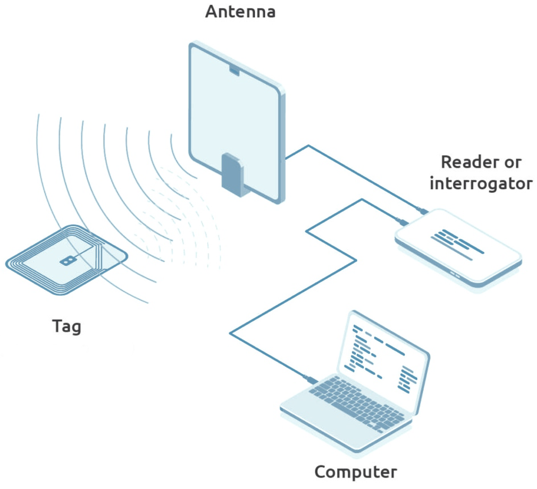
2. The RFID Technology

Generally and commercially, the RFID technology permits, automatically, the identification and/or the storage of data relating to objects [55,56,57] since it is based on the storage capacity of information regarding the object to which electronic labels (tags or transponders) are coupled. These tags are remotely interrogated by devices called readers. Over the years, RFID technology has developed and has been used in many sectors: industrial, automotive, medical, e-Government (see passports, identity cards, etc.), transport, and other uses. This technology allows the development of a reliable system of interconnected objects that collects and processes data in a single large global network (i.e., the Internet of Things). Given its versatility, it is considered a general-purpose technology.
An RFID system mainly is composed of four main parts:
  • A tag, which is composed of an antenna and an integrated circuit (IC) that has simple memory and simple control logic functions and is packaged as a plastic or paper label. The tag is powered up by other elements of the system through an electric or magnetic field, then it is able to transmit the information that contains. Reading and writing are allowed in handling such information in the tag memory, which stores a unique identification code.
  • The battery-less microchip inside the tag receives power through electromagnetic waves that are collected by the antenna of the RFID tag, then it allows the sending and receiving of the data contained in the memory by modulating the field back-scattered by the antenna.
  • The reader, the device used to interrogate tags also reads and filters the information back-scattered from the tags. Readers can include their own antenna in an integrated structure or can use a distinct antenna.
  • The management system (server, host computer) acts as an information interface between the reader and the network. It allows us to obtain all the available information associated with tagged objects, the identification codes of each tag, and to manage the whole system for the purposes of the use case.
Figure 1 is represented by an RFID system with its components.
Tags are classified into three main groups: Passive, Active, Semi-Active, or Semi-Passive. Moreover, they can vary in size, shape, material, and operating frequency.
In this study, we make use of passive UHF-RFID tags, they do not have a battery but they take energy from the electromagnetic signal sent by the antenna of the reader.
In the far-field region, the interaction of the components is dominated by the electromagnetic field created by the antenna. The RFID tag resonates with the frequency of the electromagnetic field and the current generated activates the chip. The UHF class of tags operates at 867/868 MHz with distances up to thirty meters.
In this research, we used “LabId UH105” RFID commercial tags to check the displacements of two brick walls 1 m wide and 2.70 m high that underwent out-of-plane forces provided by a concentrated load acting along the middle of each wall. The application of this type of sensor in civil engineering can be considered an innovation for this kind of research since no literature reports similar applications. Experimental tests were first conducted in a controlled environment (the laboratory room) to study the feasibility of the method, and subsequently conducted on-site.

3. Experimental Investigation of the Application of the UHF-RFID Tags for Structural Monitoring

The commercial UH105 passive transponder made by LAB-ID have been used (Figure 2). The dimension of each tag is 17.85 × 90.85 mm2 and it consists of a polyester (PET) substrate (38 μ m thick), an aluminum dipole antenna (9 μ m thick), and an EPC Class 1 Gen2 Impinji Monza 5 chip operating in the 840 MHz–960 MHz band, linked to the terminals of the antenna. Thanks to the good radiative properties, and specifically to the insensitivity with respect to the orientation in the space in which it is positioned, these tags can be detected at a great distance and it is suitable in situations in which there is a great number of tags, like in logistics.
Table 1 and Figure 3 report the main features of the UH105 tag.

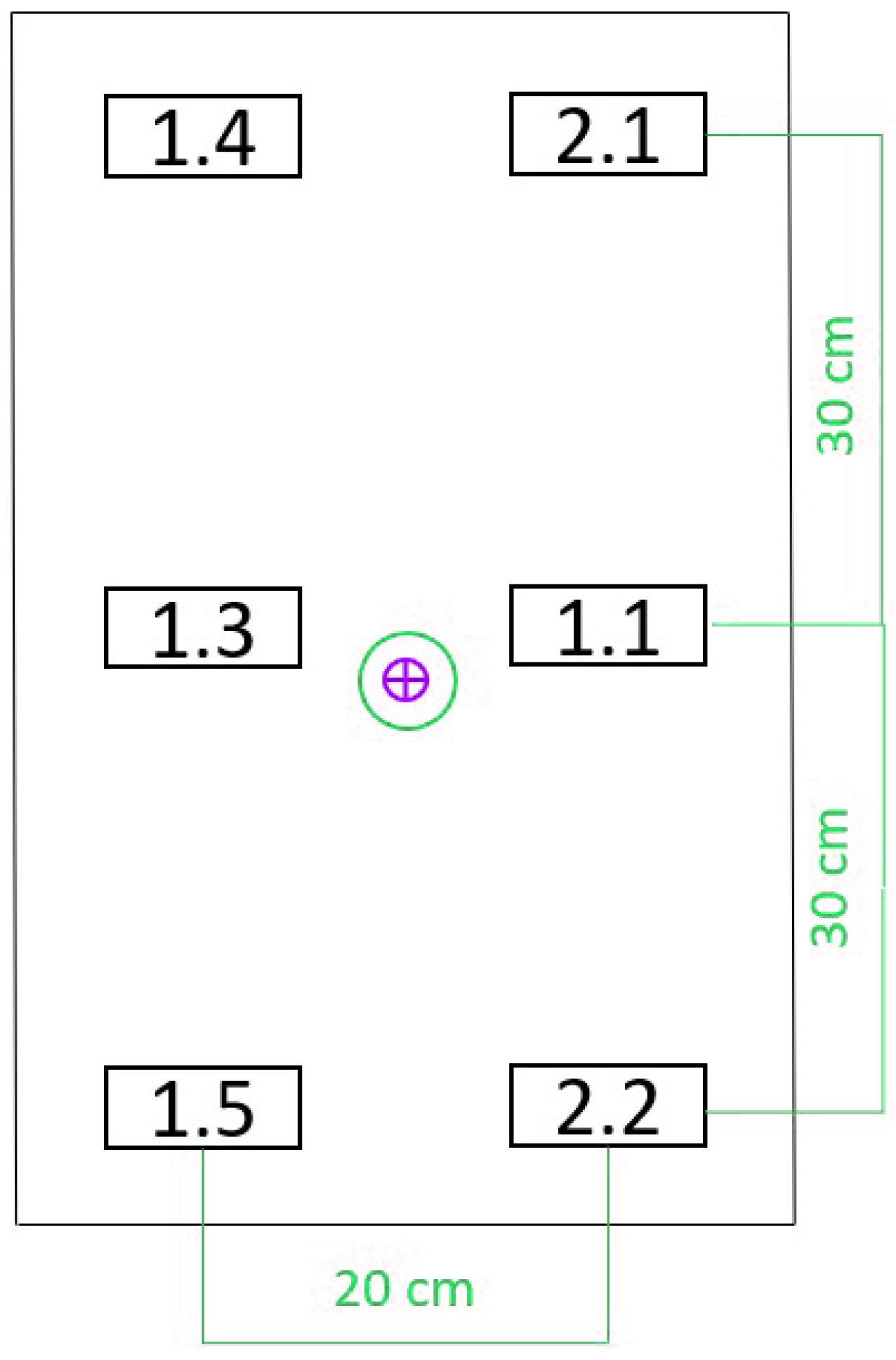
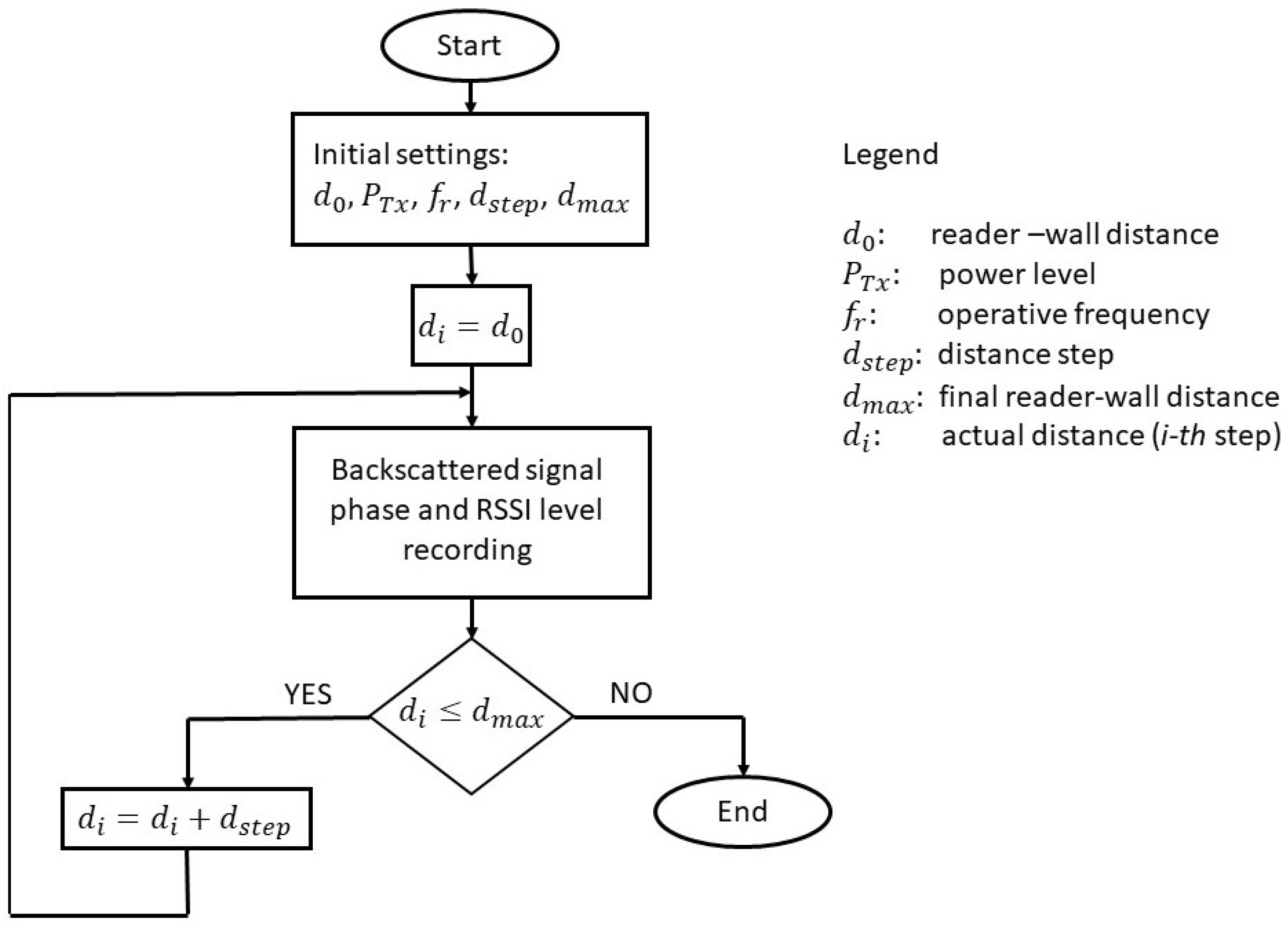
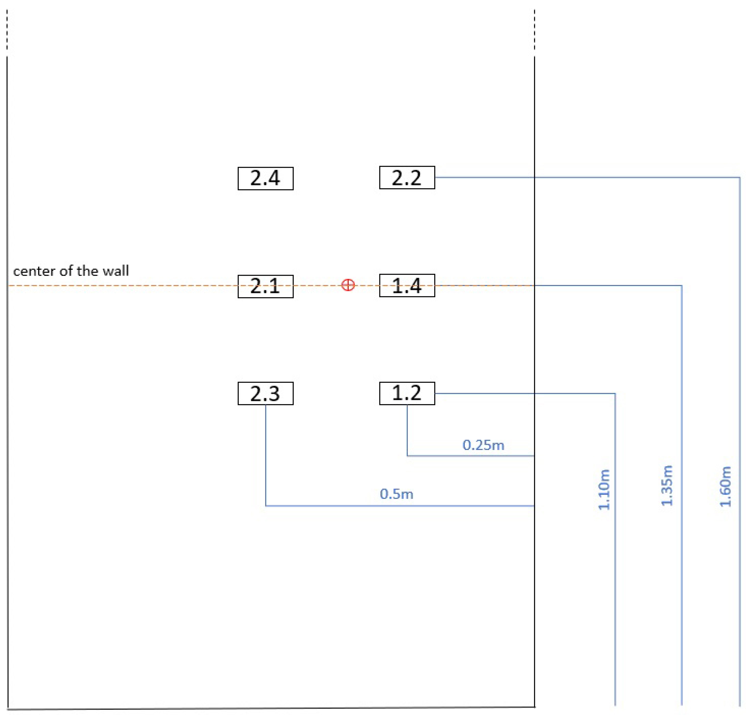
3.1. Laboratory Tests: Monitoring the Tags Displacements under Out-of-Plane Action

For assessing the feasibility and reliability of UHF RFID tags in monitoring out-of-plane displacements, two experimental tests were carried out in a laboratory environment.
In order to compare secondarily the laboratory results and the in situ experimental results, the same configuration of tag position, measurement distances, and spaces were designed and applied to the in situ experimental set-up of each test, so that laboratory and in situ tests would have the same boundary conditions, except for the environment.
The first laboratory test set-up was composed of six tags positioned following a 3 × 2 grid. Each tag was identified by an ID number, so they were identified as Tag 2.2, Tag 1.5, Tag 1.1, Tag 1.3, Tag 2.1, and Tag 1.4.
The authors decided to position the tags on a polystyrene panel since polystyrene results “transparent” to the electromagnetic waves so it does not influence the back-scattered signal. The position of the tags is shown in Figure 4. The reader’s antenna was placed in front of the polystyrene panel, with a distance greater than 60 cm. The center of the reader’s antenna (represented as a projection by a violet dot in Figure 4) appears on the panel at 3 cm (approximately) below the central row of the tags. The operating frequency is 867 MHz while the radiated power was set at 20 dBm since it was sufficient for a correct reading of each tag. A micro-metric screw was applied to the panel in order to move it orthogonal to its plane for simulating forces that cause out-of-plane displacements. The displacements were performed by moving the panel at steps of 5 mm, reaching 60 mm of distance from the starting position.
A second laboratory experimental test was performed, with a similar set-up. The tags chosen for the 2nd experimental test were: Tag 2.4, Tag 2.2, Tag 2.1, Tag 1.4, Tag 2.3, and Tag 1.2.
Only a few tags were chosen for both laboratory tests in order to not overlook any anomalies related to the specific characteristics of a given tag.
The tags were positioned on a polystyrene panel, as represented in Figure 5. The reader’s antenna was placed in front of the panel, at 62 cm of distance. In this case, the projection of the center of the reader’s antenna on the panel (dot in violet in Figure 5) results at 15 cm from the center of Tag 2.1 and 10 cm from the center of Tag 1.4. The panel was subjected to the same out-of-plane displacements of the 1st test (orthogonal to the panel) with steps of 5 mm, by the use of a micrometric screw, reaching 70 mm of maximum distance compared with the starting 0 position. In this case, the radiated power was set at 24 dBm, which ensured a correct reading of each tag. The test set-up is shown in Figure 6.

3.2. Results of the Laboratory Experimental Tests

In both laboratory tests, the measurement system recorded the displacement at each step (each 5 mm). The quantities useful to determine the displacement are the phase and RSSI (“Received Signal Strength Indicator”) of the signal backscattered by tags and received by the reader. The results of the displacement measurements are reported for each tag, determining the mobile mean and standard deviation of the phase, for each step of measurement. The RSSI is also reported. Values around −52 dBm shows a good signal’s quality.

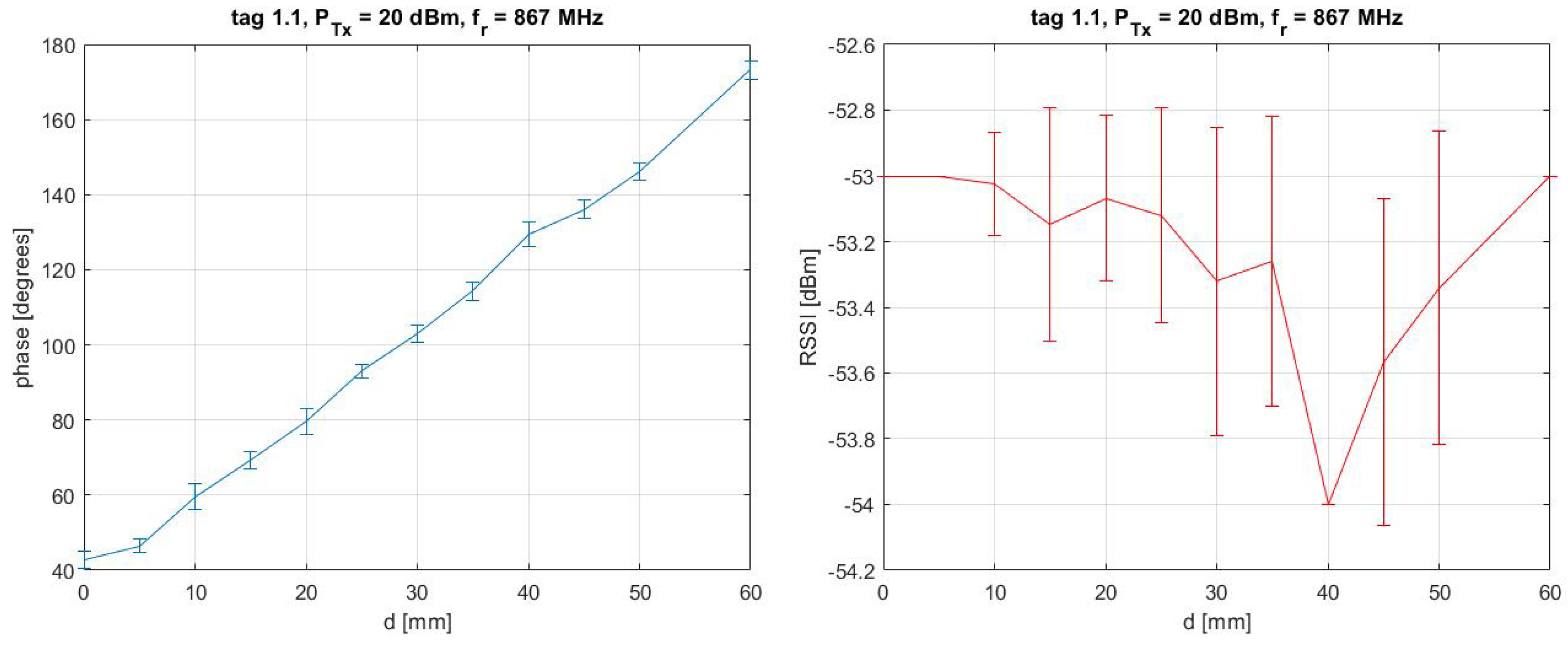
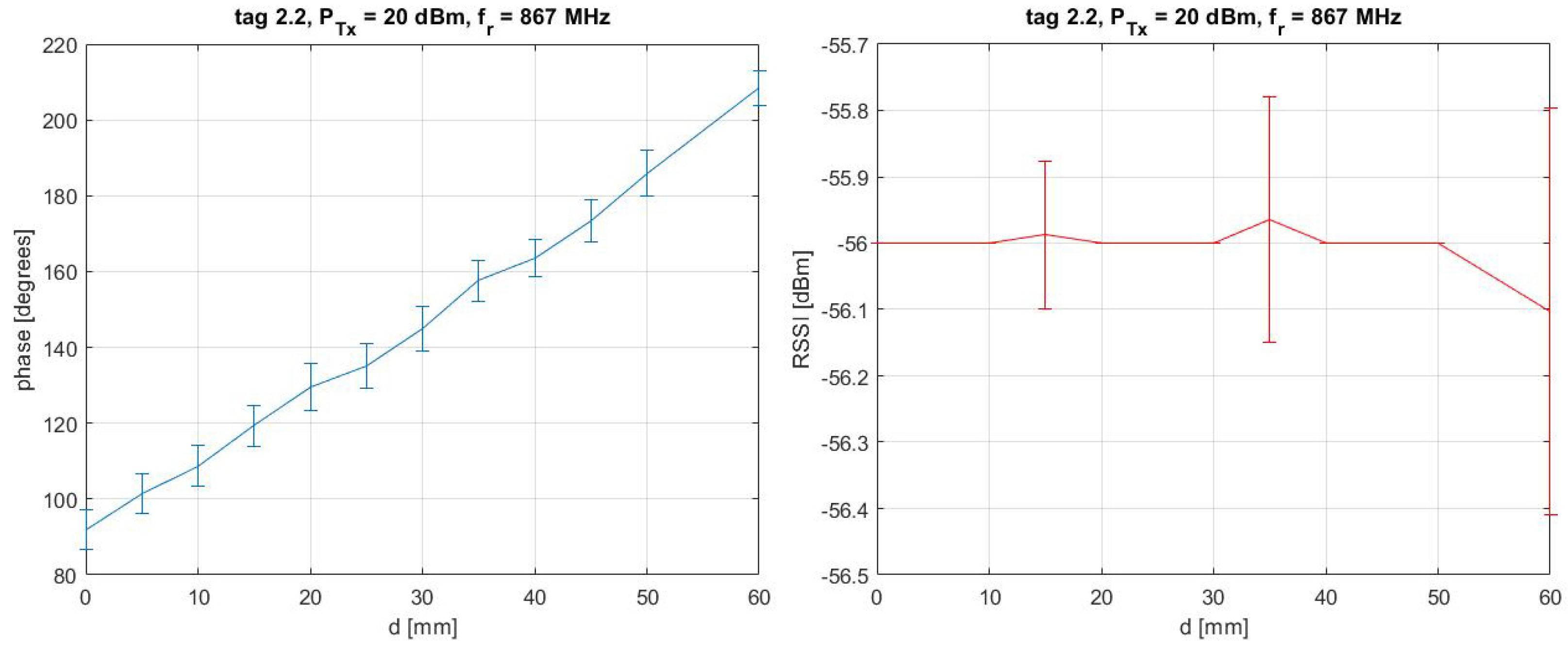
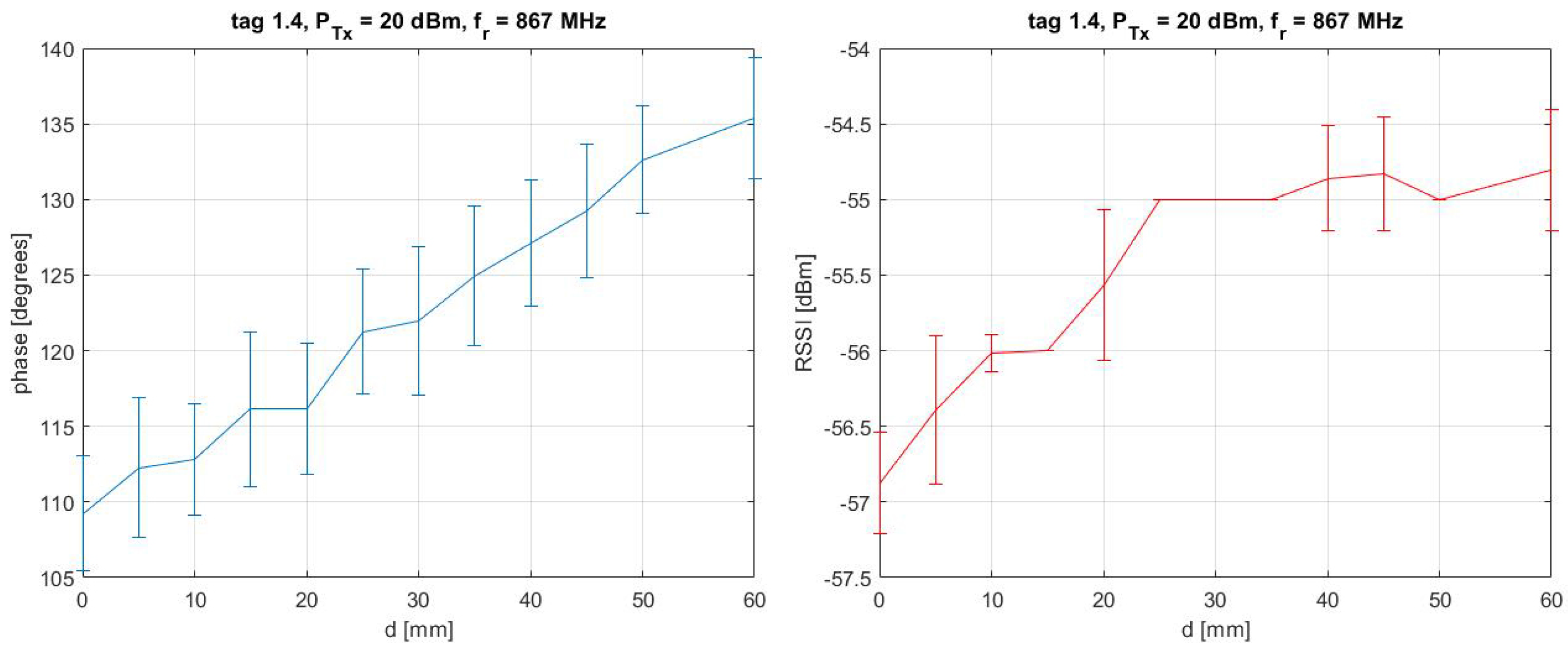
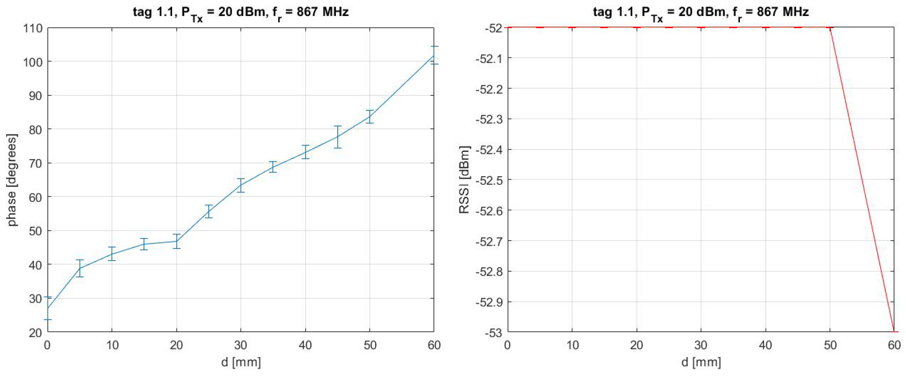
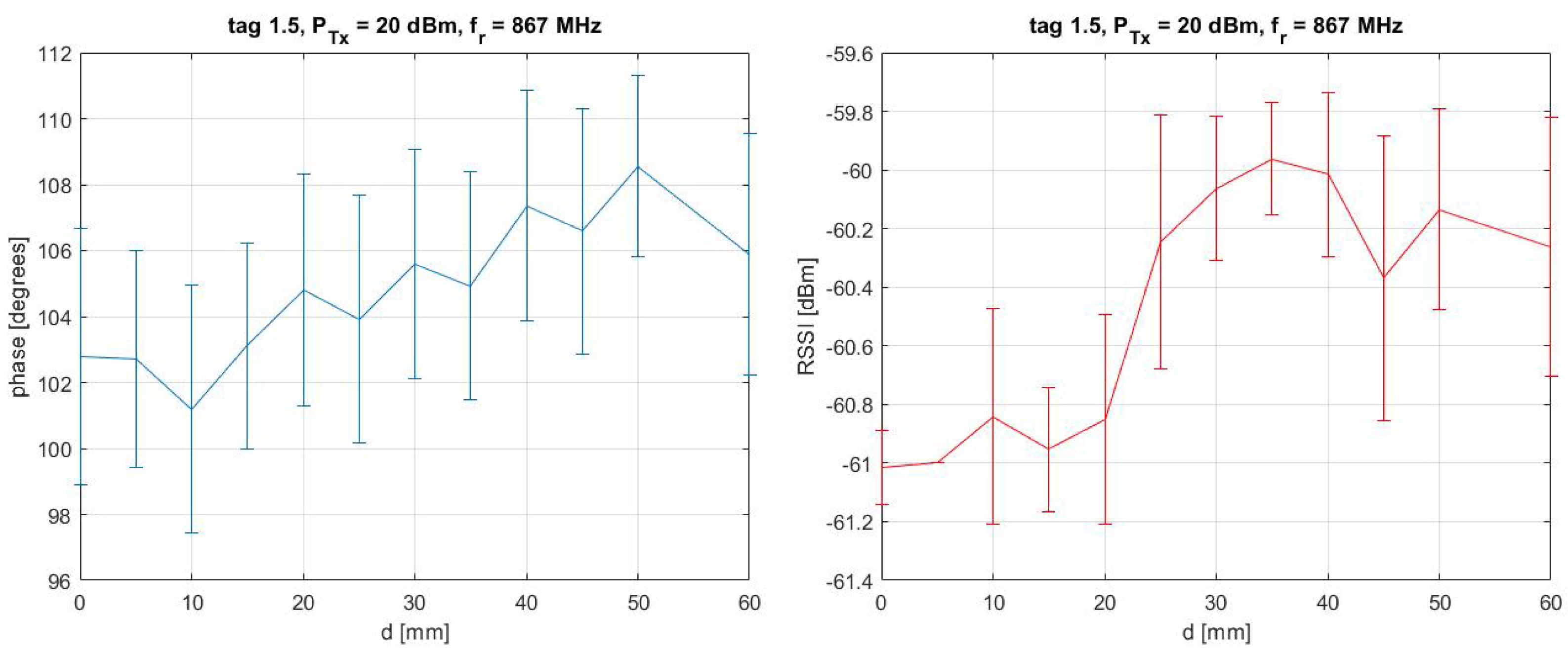
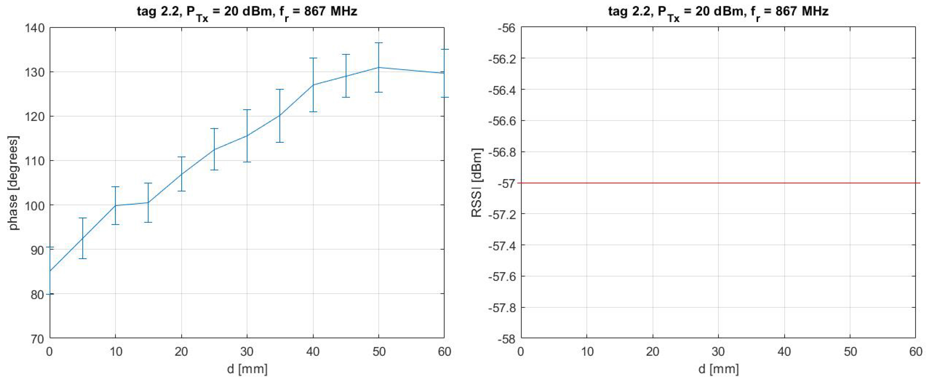
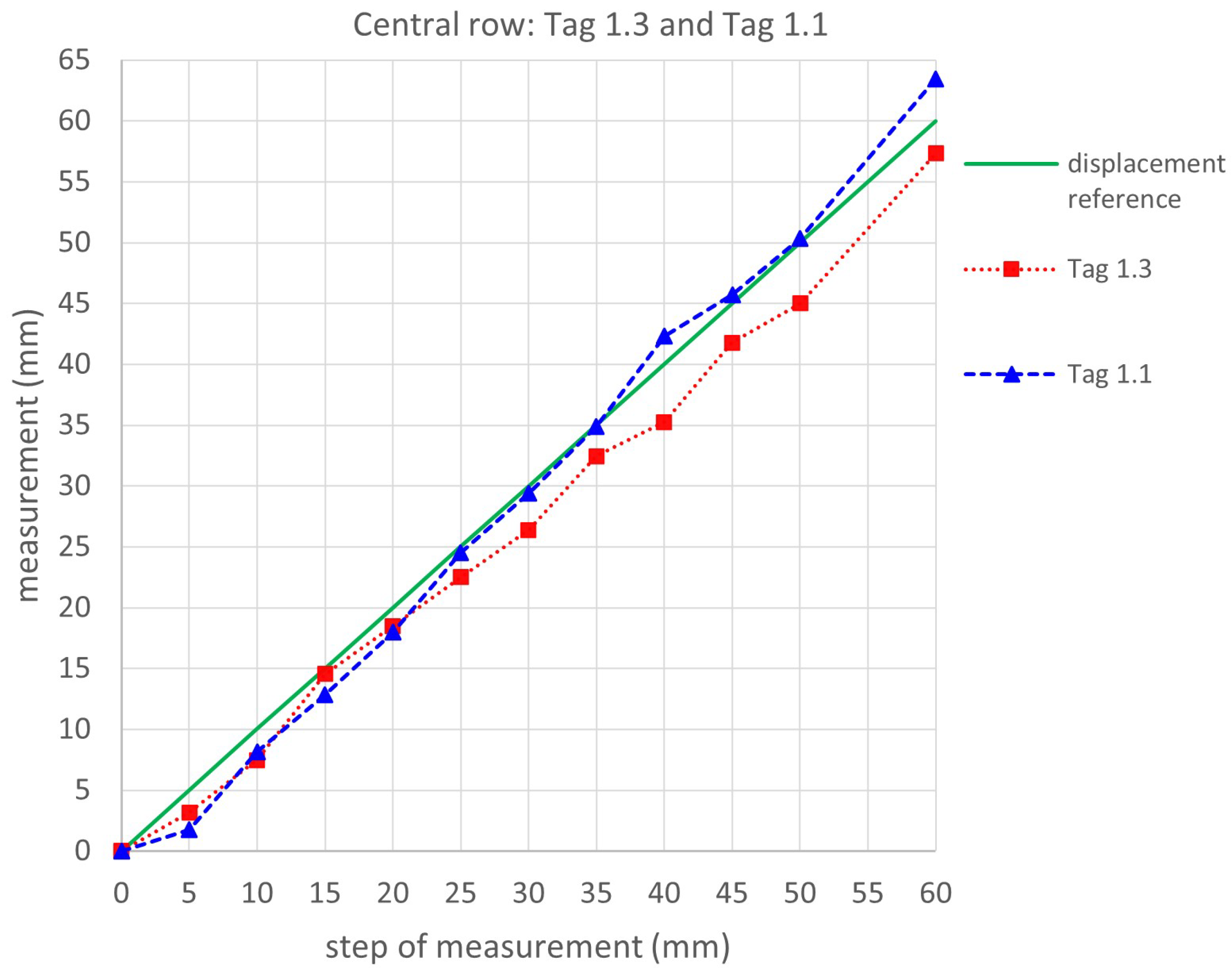
3.2.1. Results of the 1st Laboratory Test

In Figure 7, Figure 8, Figure 9, Figure 10, Figure 11, and Figure 12, the results of the acquisition systems of Tag 2.2, Tag 1.5, Tag 1.1, Tag 1.3, Tag 2.1, and Tag 1.4 are reported, respectively. The values of the mean and standard deviation of the phase recorded at each step of measurement, and RSSI values, are reported for each Tag.
Evidently, the values of phase change pass from 0 mm to 60 mm. In detail, values of phase are increasing passing from one measurement step to the successive (from Figure 7, Figure 8, Figure 9, Figure 10, Figure 11 and Figure 12). This demonstrates that tags are sensitive to the displacements imposed on the panel. For Tags 1.4, 1.5, and 2.2, the RSSI values are quite constant (meaning stale communication), while for the other tags, RSSI values show very small fluctuations, which are acceptable.
In Figure 13, a flowchart illustrating the methodology used to obtain the results is represented.
The assessment of the feasibility of this new wireless monitoring system can be achieved by converting the phase difference between two consecutive measurement steps into distance difference (which should be related to the imposed displacement) by using the following equation:
d d 0 = ( f f 0 ) · λ 4 · 180
where f f 0 is the difference in phase between a specific step of measurement and the previous step, and λ is the wavelength of the electromagnetic signal that is 0.346 m in this specific case.
From Equation (1), we determine the difference in distance d d 0 that occurs when the panel or the tag moves from one position to another.
This distance measured by the tags does not correspond to the displacement we are interested in knowing, i.e., the measured distance concerns the slant path between the reader’s and tag’s antenna while we are interested in the movement (out-of-plane) along the direction orthogonal to the plane on which the tag is placed. For this reason, the out-of-plane displacement was calculated geometrically projecting the measured slant path onto the orthogonal direction by exploiting the knowledge of measurement set-up.
In order to assess the feasibility of the proposed technique we compare the results of the displacements measured by the tags with the actual displacements imposed (indicated as “displacement reference” in the following graphs).
For faster comprehension, the comparison of displacements has been shown according to the position of the tags (see Figure 4).
Figure 14 shows the displacements measured by Tag 2.1 and 1.4, compared to the displacements imposed on the panel. Figure 15 shows the displacements measured by Tags 1.1 and 1.3 and Figure 16 shows the displacements of Tags 2.2 and 1.5.
All the tags show almost matching displacements, as can be seen from the graphs. Considering the standard deviations of the values calculated using the phase measurements and the intrinsic measurement errors of the reader itself, this represents a surprising result.
It should be considered that, generally, RFID tags are influenced by metals since the electromagnetic waves are strongly scattered by metallic objects. Specifically, tags reflect part of the electromagnetic power received from the reader, this phenomenon is known as “back-scattering”. Metal objects around the tag can modify or screen the signals exchanged with the reader, it is undesired in our experiments since it corrupts the expected results as shown later on. For this reason, experiments were performed initially in a laboratory room where no metals or other obstacles were detected.
In this experiment, a higher error is observed for the upper row tags, in particular for Tag 1.4.
The cause of higher error is supposed to be the larger distance of the reader’s antenna from the corresponding tags with respect to central and lower row tags (see Figure 4). Tags in fact are placed on a rigid panel that translates rigidly so that their out-of-plane movement should be the same. Hence, the resulting discrepancies could be due to the environment since Tag 1.4 is located close to a plasterboard wall of the laboratory. We suppose that the metallic frame of the plasterboard wall has affected the signal, modifying the tag’s response. Tags 1.5 and 1.3 (see Figure 6) also have a distance from the plasterboard wall as that of tag 1.4 but their response is better, they probably suffer less from the frame of the wall.

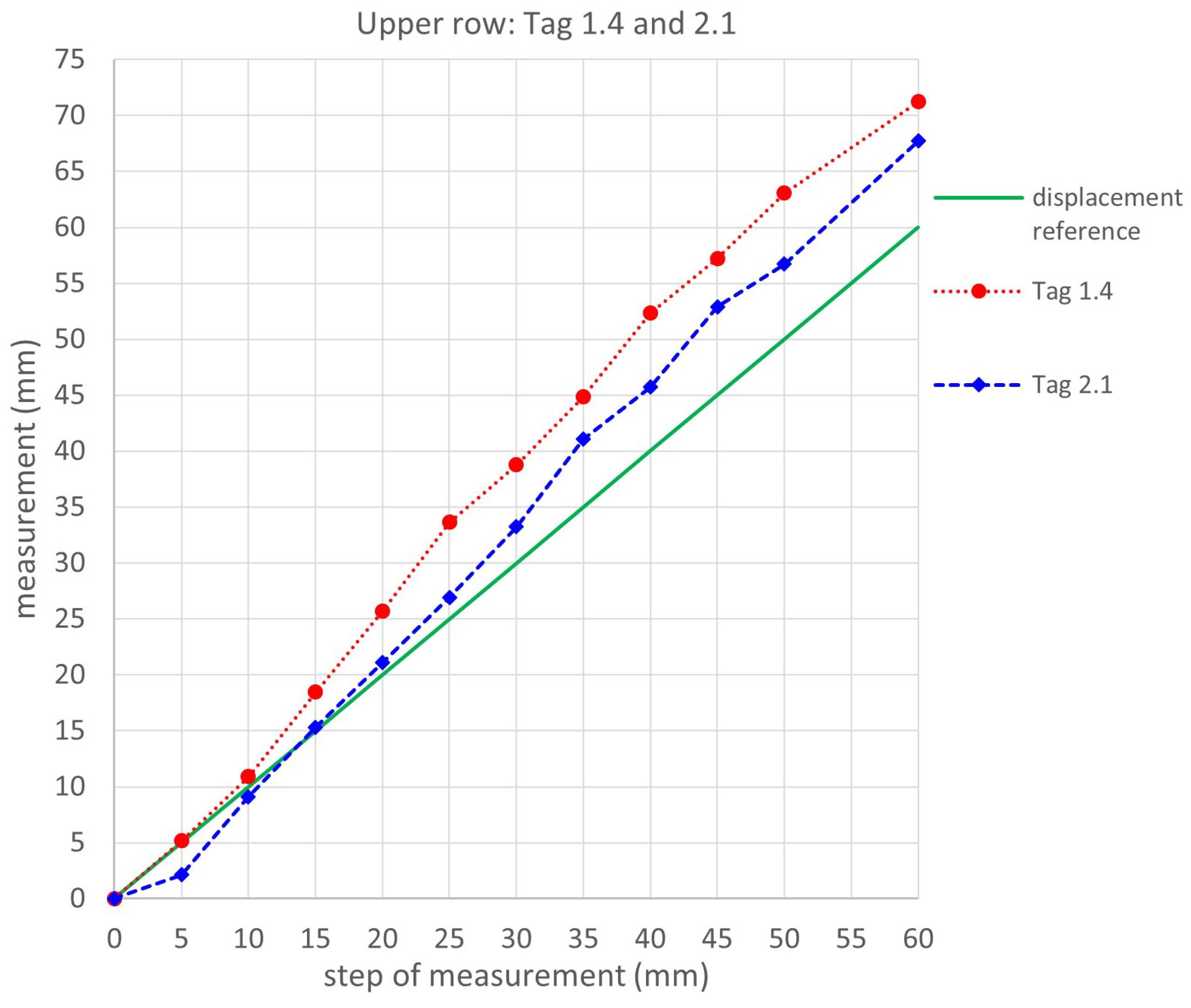
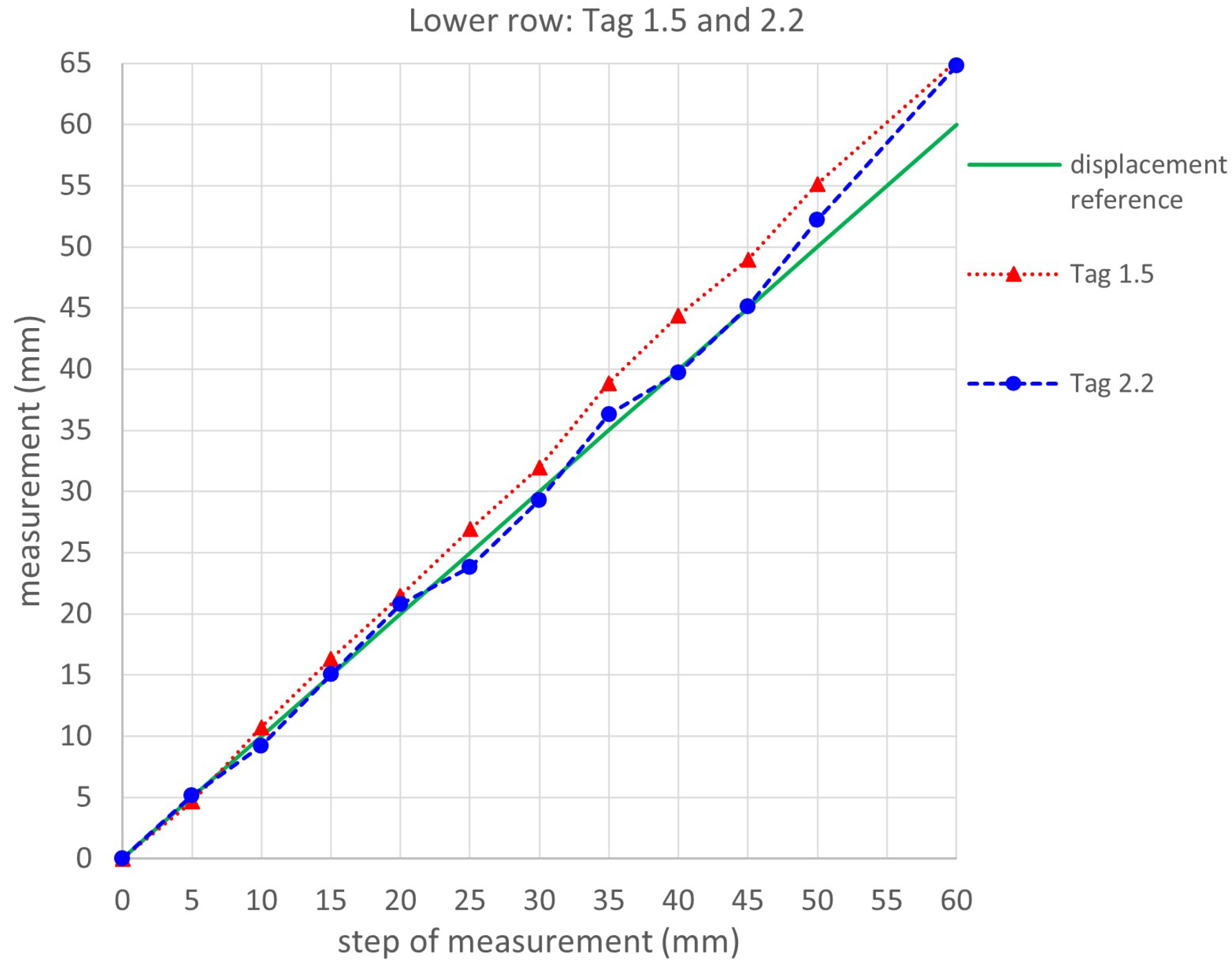
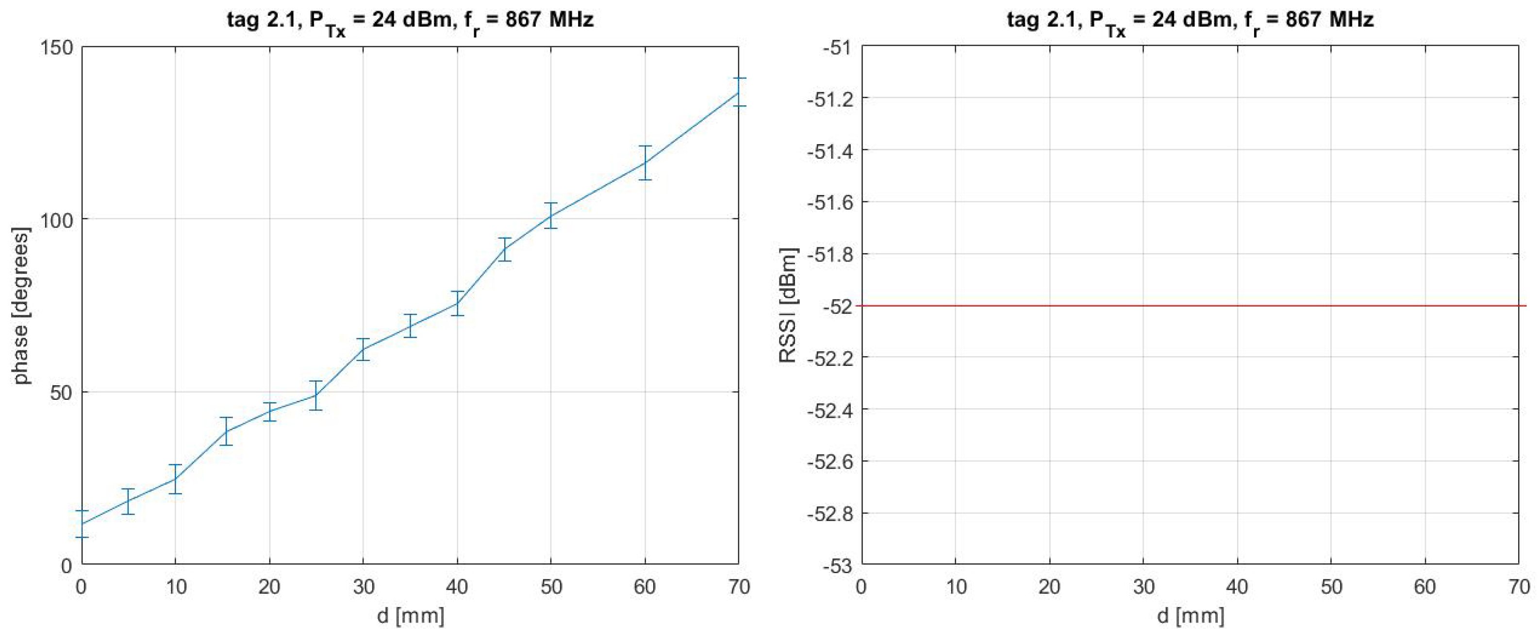
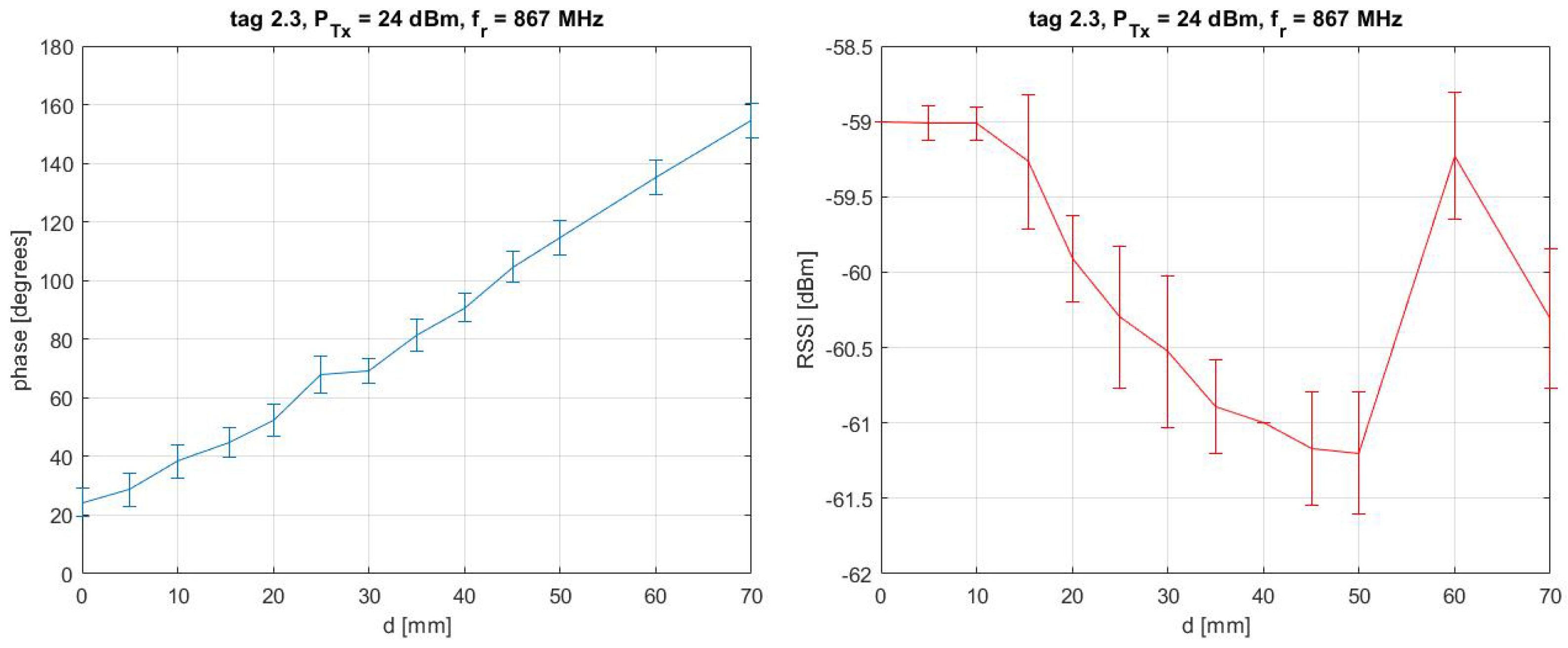
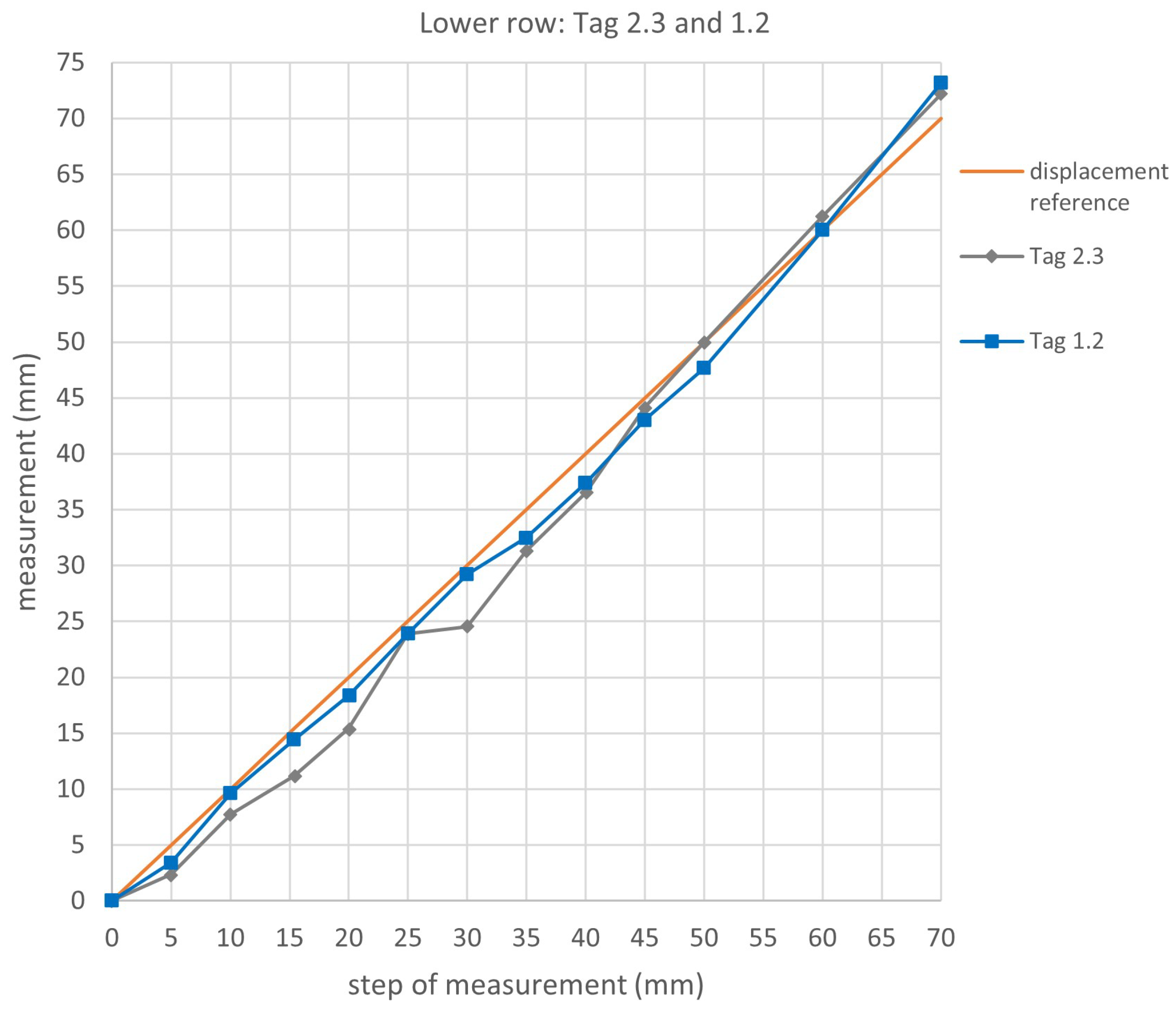
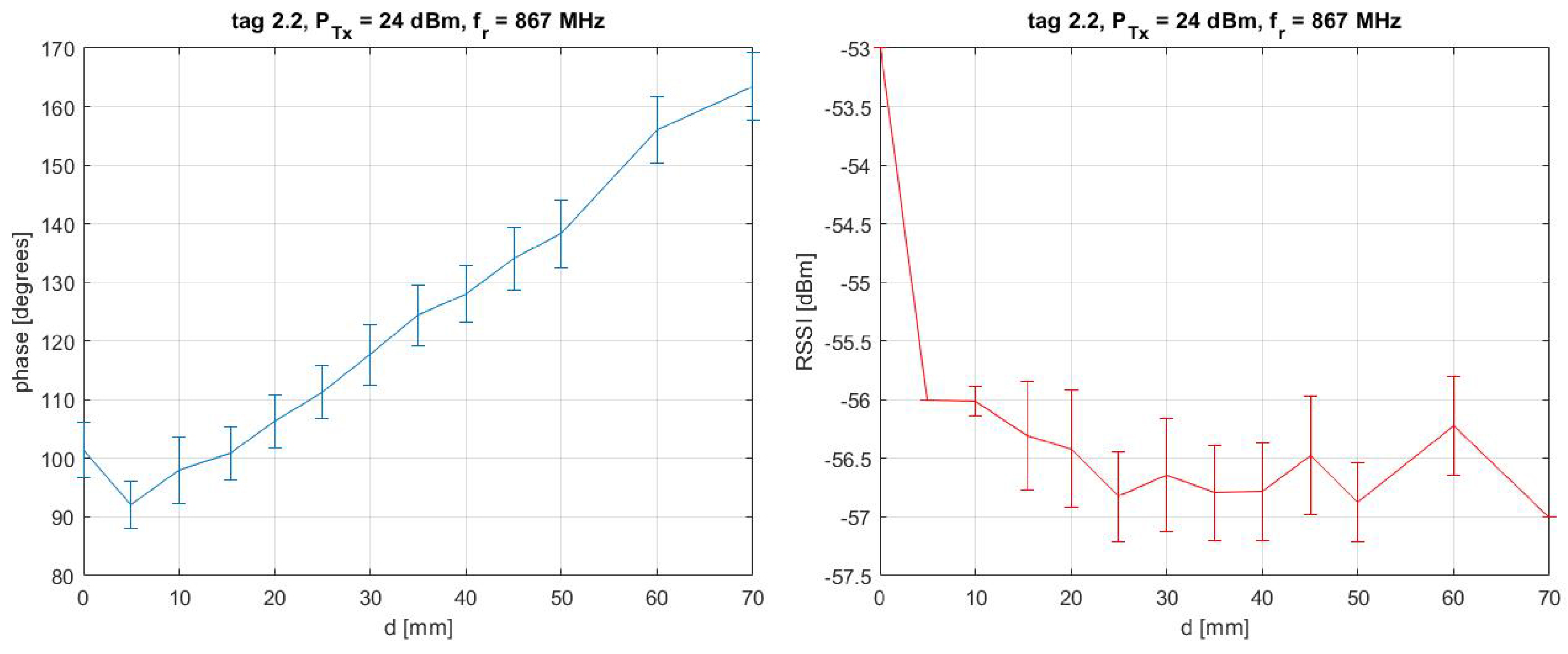
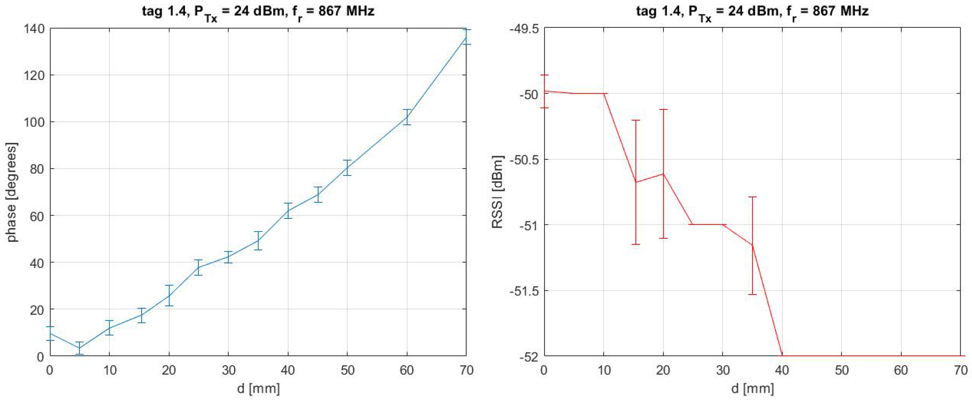
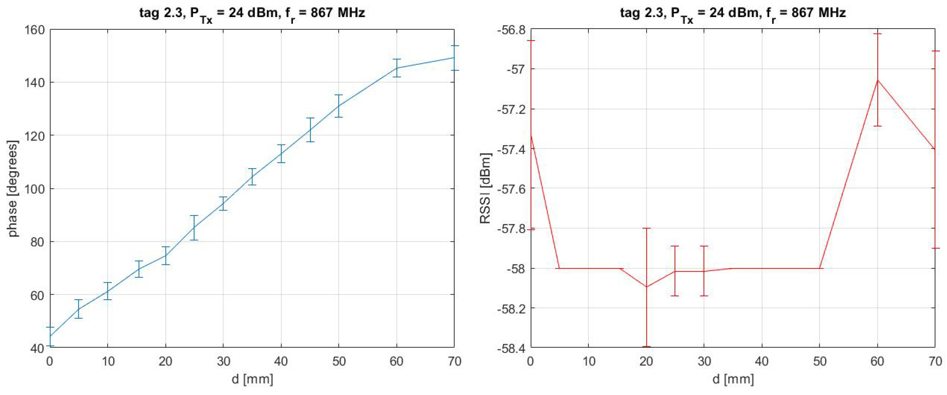
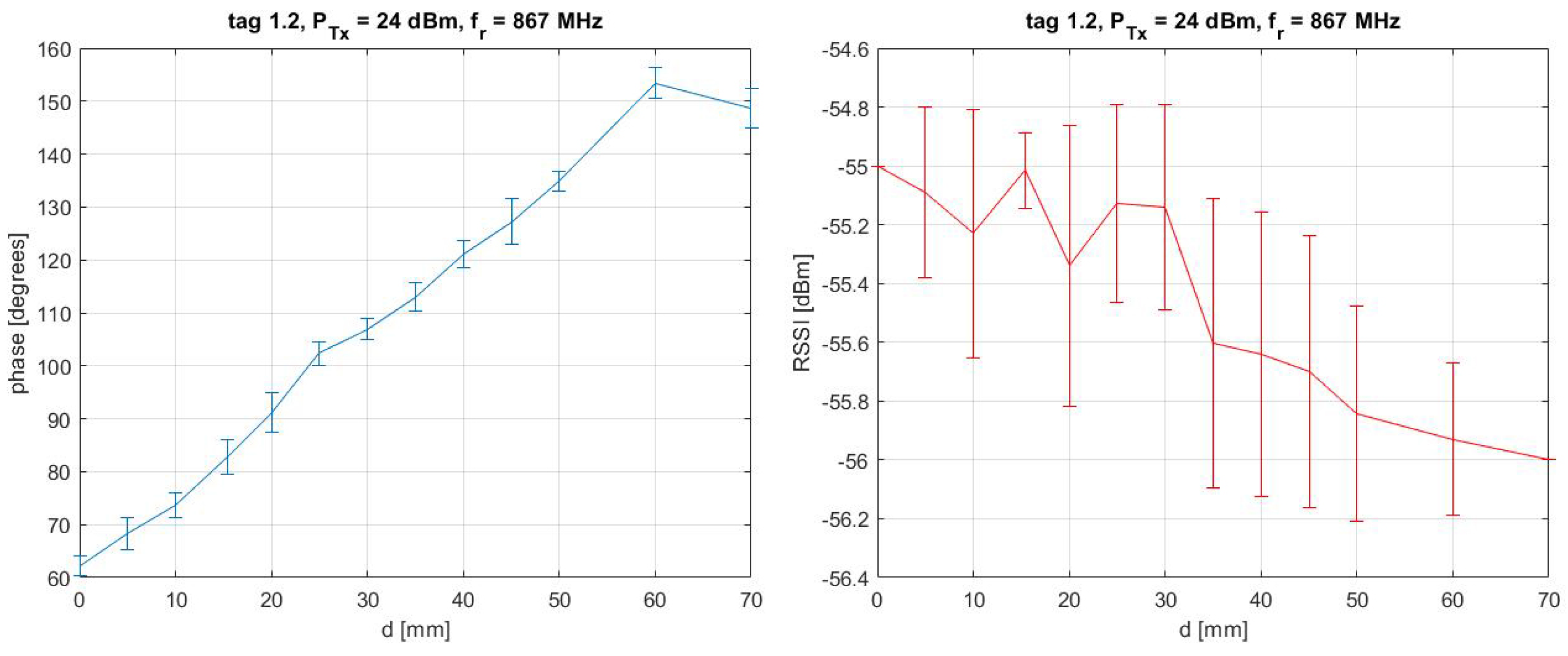
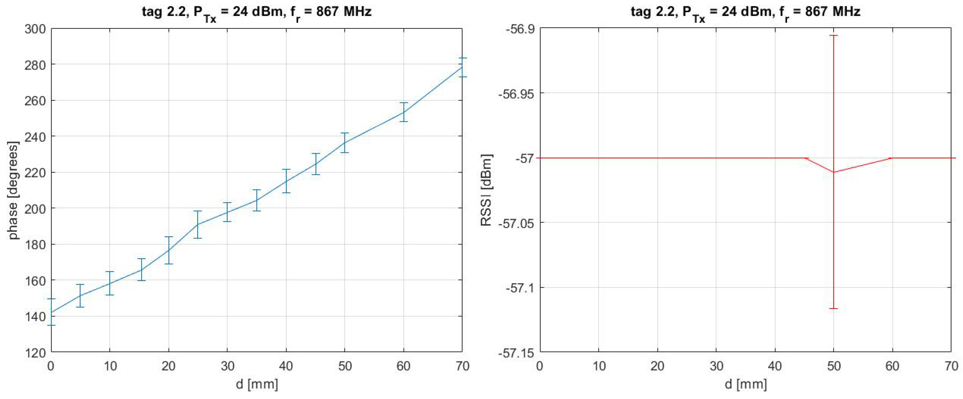
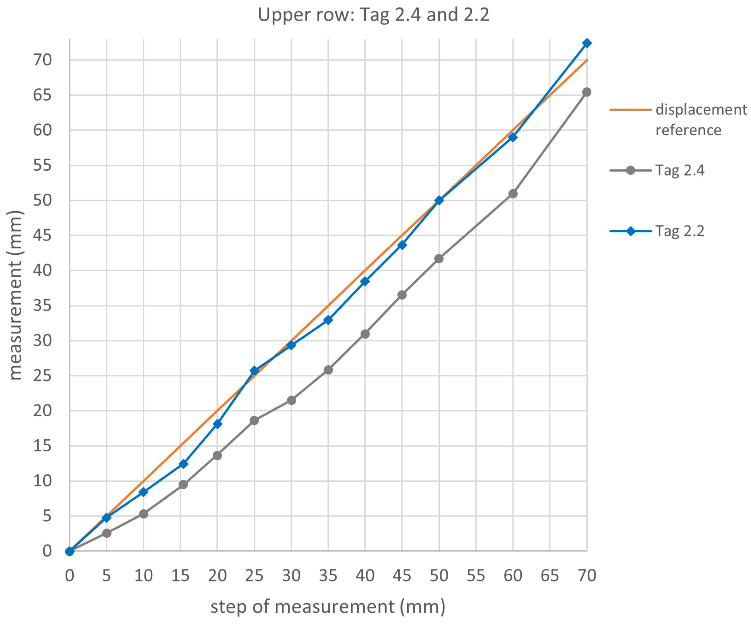
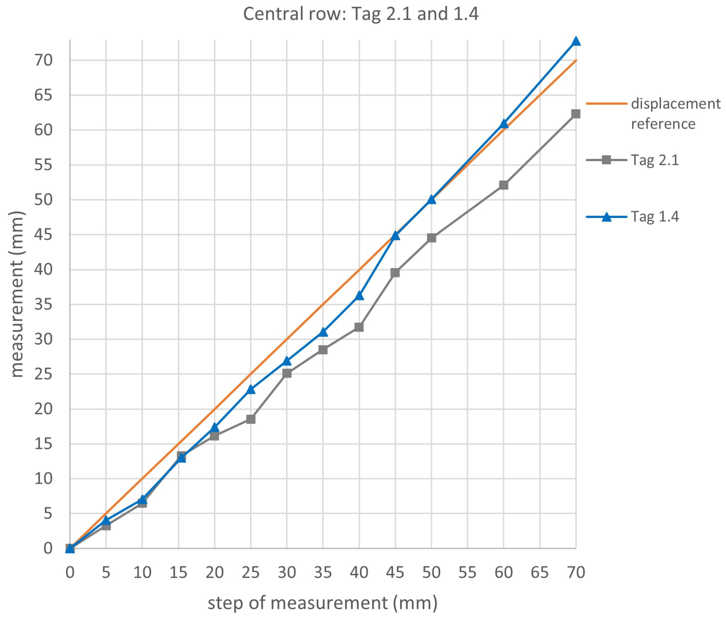
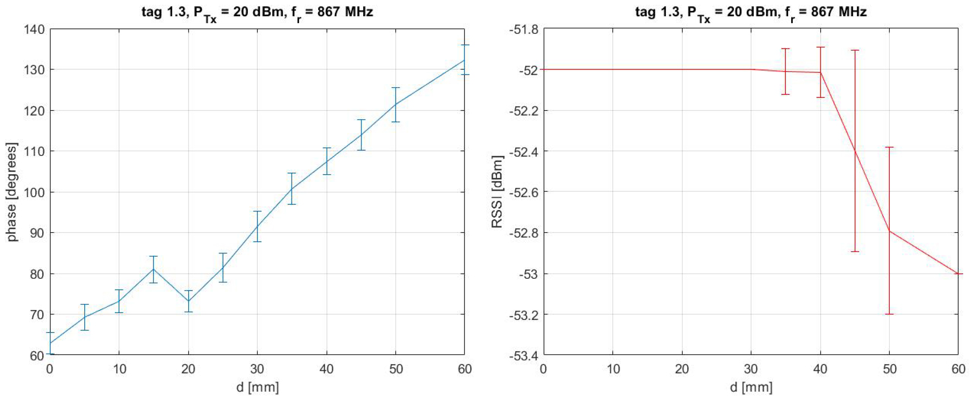
3.2.2. Results of the 2nd Laboratory Test

In this second test, the same Tags 2.1, 1.4, and 2.2 were used together with new Tags 2.4, 2.3, and 1.2.
In Figure 17, Figure 18, Figure 19, Figure 20, Figure 21, and Figure 22 the results of the acquisition systems of the Tag 2.4, Tag 2.2, Tag 2.1, Tag 1.4, Tag 2.3, and Tag 1.2 are reported, respectively. The values of mean and standard deviation of the phase recorded for each step of measurement, and RSSI values, are reported for each Tag.
As can be observed from the graphs, the values of the phase increase for increasing displacement: from the starting point (0 mm) to the final point (70 mm) (see from Figure 17, Figure 18, Figure 19, Figure 20, Figure 21 and Figure 22). The RSSI values are acceptable. They are constant for Tags 2.1 and 2.2, and present small fluctuations for the other tags.
To assess also, in this case, the feasibility of the proposed wireless monitoring system (and so consider it definitely feasible), the phase differences have been converted into distance differences by using Equation (1) and the displacements of the tags in the out-of-plane direction have been geometrically calculated by a 3D modeling.
Similarly to the previous test, we compare the results of the displacement measured by the tags with the displacements imposed using the micro-screw (indicated as “displacement reference” in the following graphs).
The comparison of displacements has been shown according to the tag’s position (see Figure 5).
Figure 23 shows the displacements measured by Tag 2.2 and 2.4 compared with the displacements imposed. Figure 24 shows the displacements measured by Tag 1.4 and 2.1 and Figure 25 shows the displacements of Tag 1.2 and 2.3.
As can be seen from the graphs, the tags all show quite matching displacements. More in-depth, we can observe that the tags that are positioned to the right (Tag 2.2, Tag 1.4, and Tag 1.2) are those that better match the real displacements. Actually, these tags detected the displacements almost perfectly. This could be due to the nearer presence of the antenna (see the projection of the center in Figure 5). The tags positioned to the left are those that present higher errors, except for Tag 1.2. It can be supposed that the reduced response of these tags is due to their position, which is more distant from the antenna, together with the influence of the plasterboard wall.
Overall, it can be observed that:
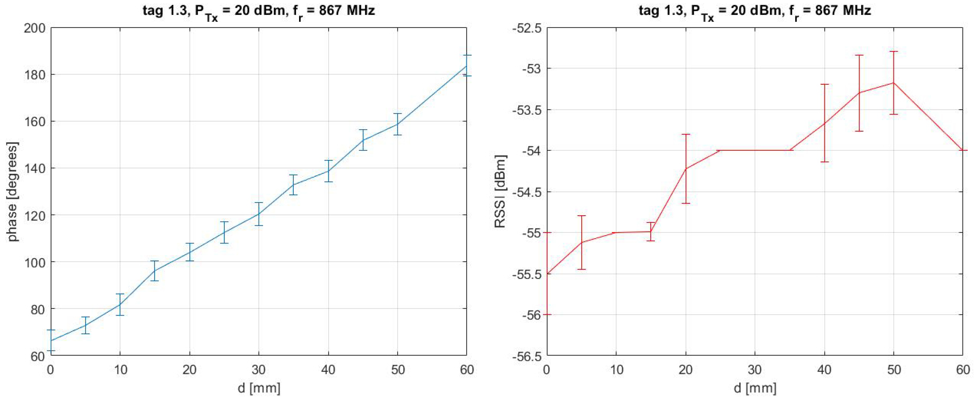
  • The displacements detected by the tags quite perfectly match the displacements imposed;
  • The altered response of some tags is due to interference in the environment and also to the more distant position of the tags in relation to the reader’s antenna;
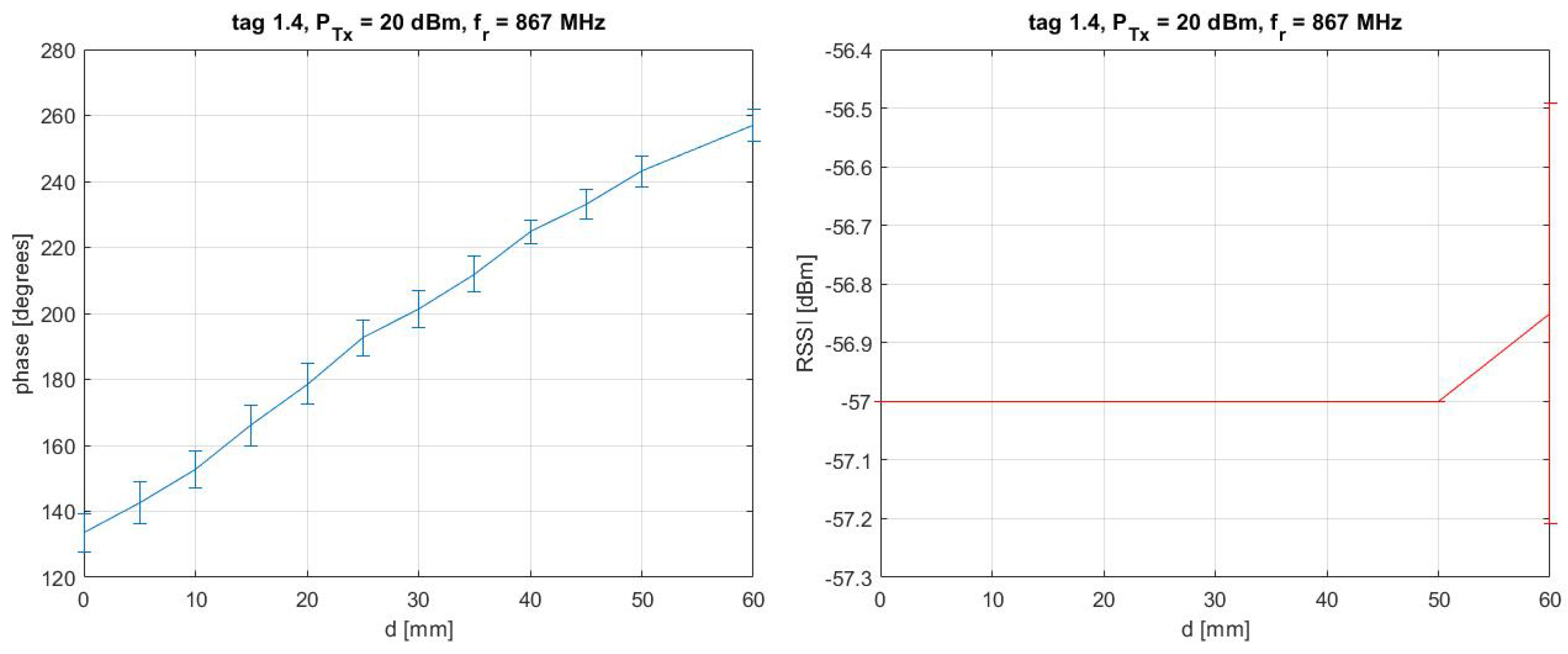
  • Measurements are intrinsically affected by the built-in errors of the reader and by the errors that occur during the processing of the data received specifically the standard deviations of the phase’s values).
For example, if we consider Tag 1.4, which has been used in both laboratory tests, in the 1st test the response of the tag is not so good because it is positioned at a greater distance from the center of the antenna (upper row) and it is near the plasterboard wall (left side). In the 2nd test, instead, the same tag is positioned in the central row (nearer the antenna) and on the right side (more distant from the plasterboard wall) and the response of the tag is very satisfactory.
We can conclude that the operation of the t in a laboratory environment is very satisfactory; thus, the innovative utilization of wireless UHF-RFID tags with the purpose of monitoring out-of-plane displacements results in being feasible and quite reliable.
Considering these results, two experimental campaigns have been performed also in situ and are described in the next section.

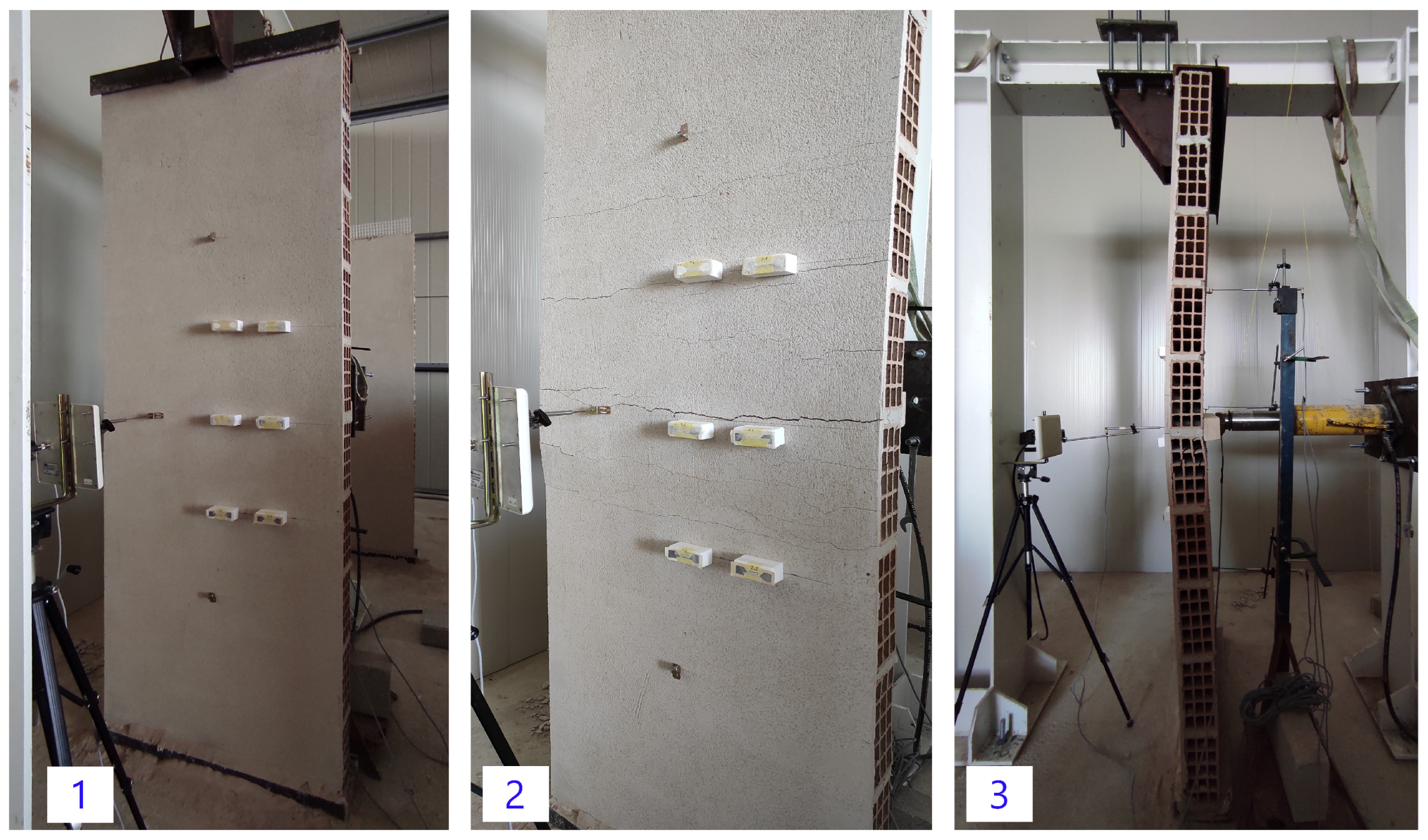
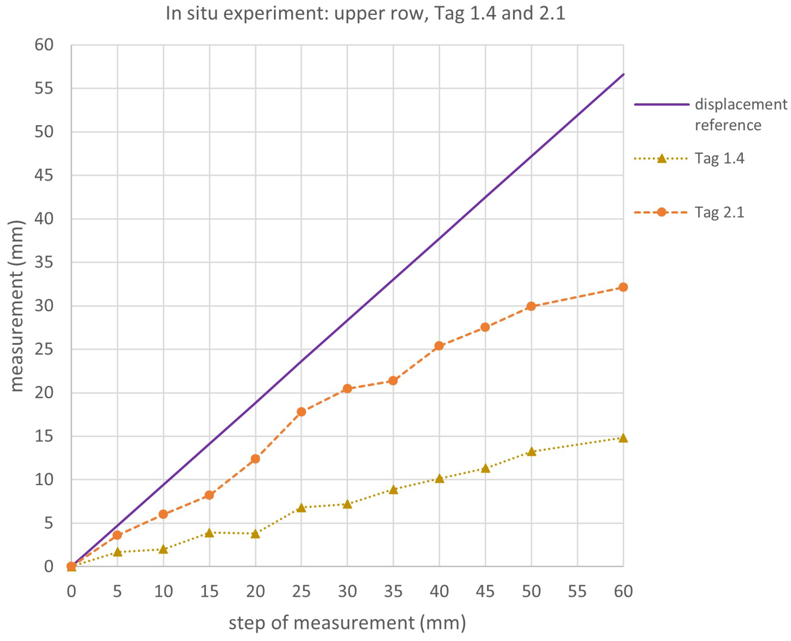
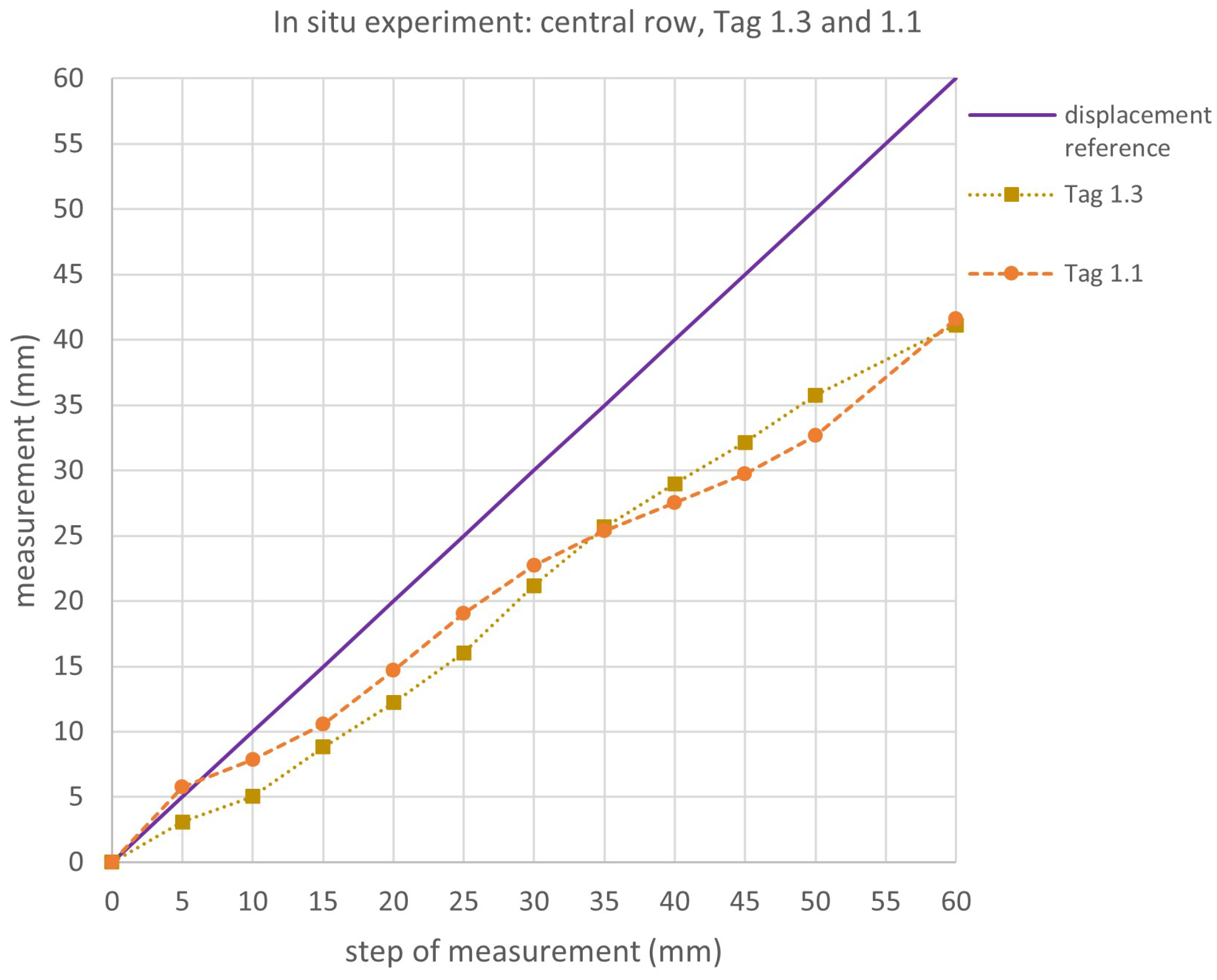
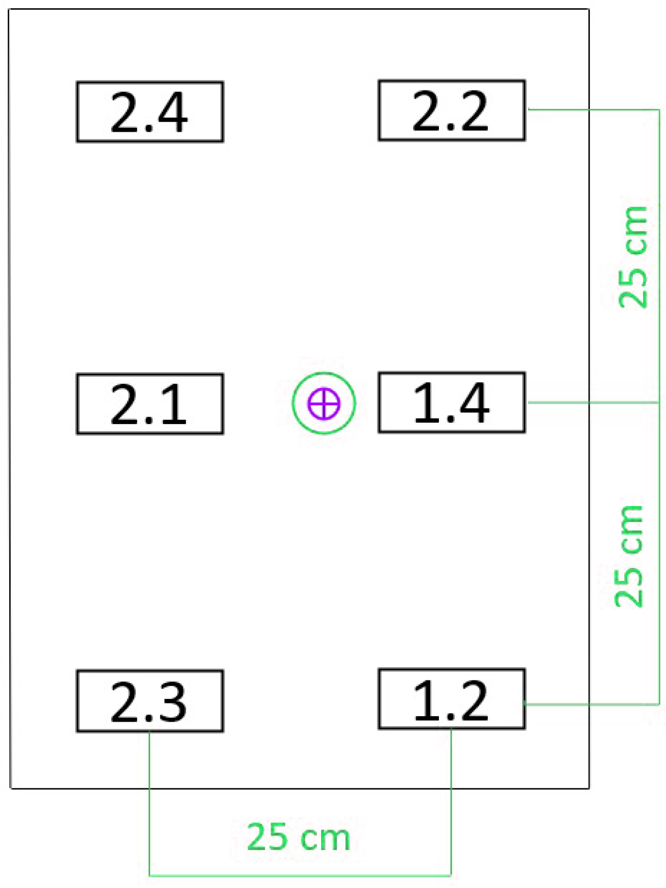
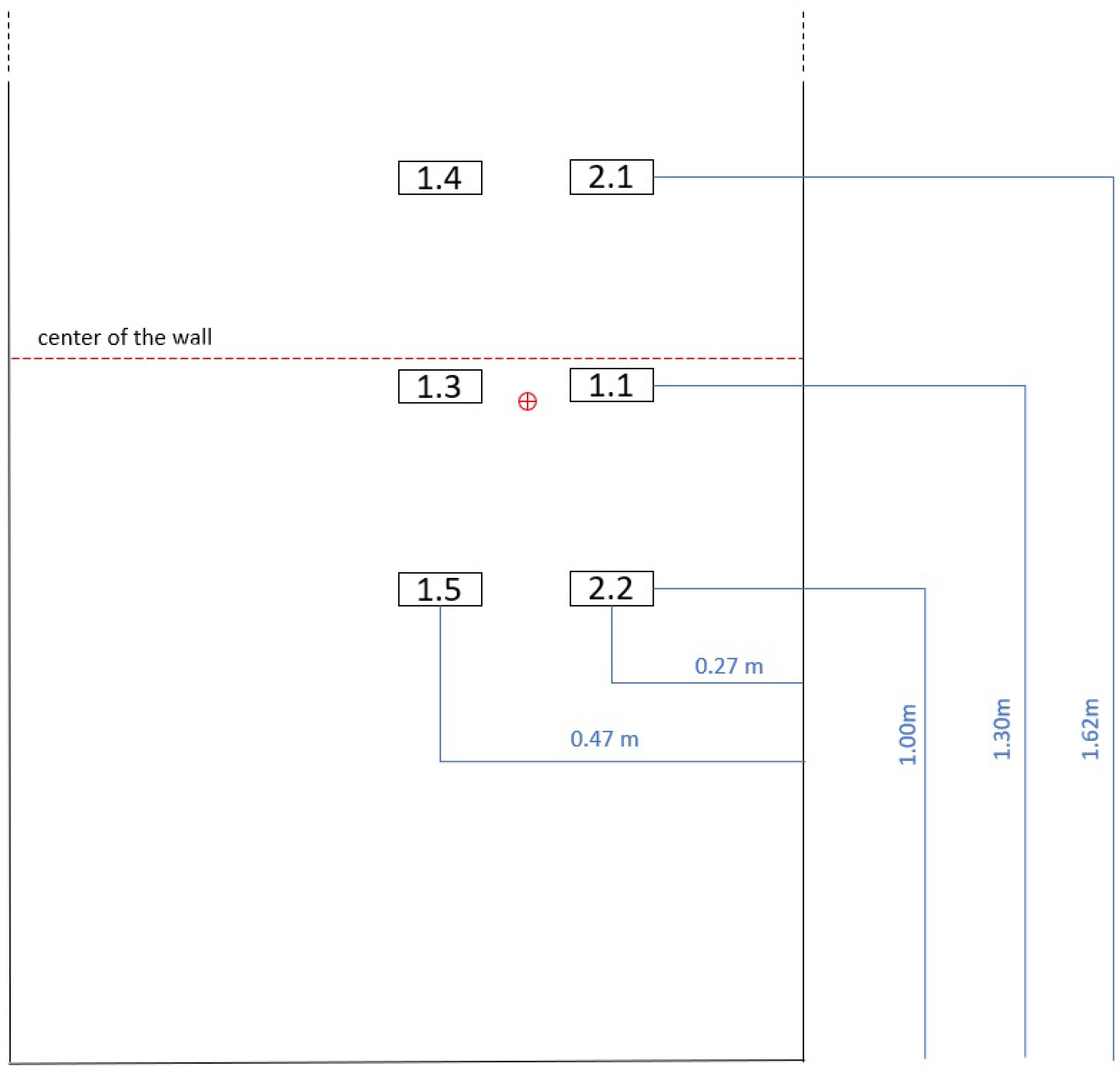
3.3. In Situ Experiments: Monitoring the Out-of-Plane Displacements of the Tags on Brick Walls

The wireless UH105 tags were used to monitor the displacements of two brick walls 1 m wide and 2.70 m high. The walls were both realized and tested on a building site. Each wall underwent an out-of-plane action caused by a concentrated load applied along the middle axis of the wall. In the set-up, each wall had a fixed constraint disposed along the entire lower side on the ground and a hinge constraint at the upper side that was anchored to the metal frame.
On the first wall, the tag’s position followed the same 3 × 2 grid used in the 1st laboratory test, in order to compare the results at the same geometric conditions. The reader’s antenna was placed at 1.27 m from the ground. The wall was 0.60 m distant from the center of the antenna. A power of 20 dBm was used for the wireless acquisition of data. The experimental set-up is reported in Figure 26.
For the 2nd wall, the same tags of the 2nd laboratory test were used. Tags were placed in a 3 × 2 grid pattern preserving the same set-up and distances. The antenna was placed at 0.62 m from the wall and at 1.35 m from ground, while the radiated power to interrogate the tags was 24 dBm. The schemes of the set-ups are shown in Figure 27.
The tags were placed on polystyrene spacers 5 cm thick in order to mitigate the electromagnetic interaction of the tag with the materials constituting the wall.
In correspondence with the expected maximum displacement (coinciding with the half of each wall and the central tags position), a wired displacement transducer was placed in order to assess the measurement. In particular, the displacement transducer was placed at a distance of 20 cm from the left-side Tag.
Compared to laboratory tests, in this case, the walls are not expected to translate rigidly since they are constrained. Consequently, the walls are subjected to deformations and the tags cannot have the same displacements as in the laboratory tests. The recording of measurements were made at each step of measurement (5 mm).
Figure 28(1) shows the set-up for the experimental test on the 1st wall. Figure 28(2) shows a detail of the tags with the deformation and cracks that appear on the wall as the displacement increases. The complete deformation and final maximum displacement are shown in Figure 28(3).
The set-up for the experimental test on the 2nd wall is shown instead in Figure 29(1) and in Figure 28(2) with a detail of the deformation and cracks.

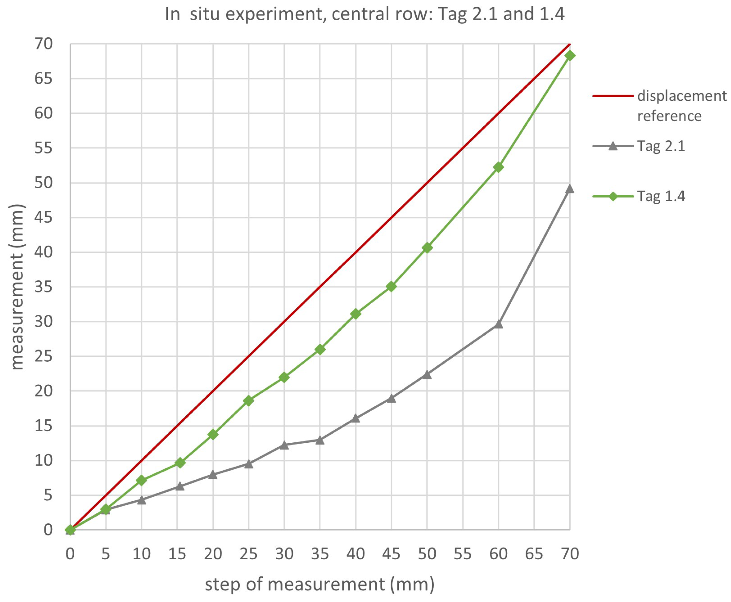
4. Results of the In Situ Experimental Tests

4.1. Test on the 1st Wall: Comparison between Wireless Tags Displacements and Displacements of the Wired Transducer

The results of the measurement acquisitions of the Tag 2.1, Tag 1.4, Tag 1.1, Tag 1.3, Tag 2.2, Tag 1.5 positioned on the 1st wall are reported in Figure 30, Figure 31, Figure 32, Figure 33, Figure 34, and Figure 35, respectively. The values of mean and standard deviation of the recorded phase for each step of measurement, and RSSI values, are reported for each tag. The variation of results mainly depends on signal-to-noise ratio, i.e., if the strength of the signal is weak the reader feels the effect of the noise more than in the case the signal is strong. Even the noise can be variable since it is a superimposition of Gaussian noise and multipath (or interference), while the former depends mainly on the quality of the used equipment the latter depends on variable environmental conditions.
As can be observed from the graphs, the values of the phase are increasing at each measurement step, from 0 mm to the maximum displacement of 60 mm (see from Figure 30, Figure 31, Figure 32, Figure 33, Figure 34 and Figure 35). The tags demonstrate a sensitive response to the displacements. The RSSI values are acceptable, quite constant for tags 1.1, 1.3, and 2.2, and with very small fluctuations for the other tags.
The detected phase differences have been converted into distance differences by using Equation (1).
The following graphs compare the displacements of the tags in the out-of-plane direction and the displacements detected by the wired transducer.
It should be pointed out that the deformation of the wall was not uniform over its surface since the wall is constrained and the deformation is caused by a load cell that imposes forces along the center of the wall pressing in the out-of-plane direction. For this reason, the measurements to consider as reference for the tags positioned up and below the middle of the wall were calculated considering a theoretic model in which the wall was simplified as a beam constrained with fixed and hinge joints on which a concentrated load is applied in the middle.
For each tag (see Figure 26), the displacement results were plotted for comparison with those calculated for the reference wired transducer.
The displacements detected by Tag 2.1 and 1.4 are reported in Figure 36 compared with the calculated displacements detected by the wired transducer (plotted as displacement reference). Similarly, the displacements detected by Tags 1.1 and 1.3 are reported in Figure 37 and the displacements of Tags 2.2 and 1.5 are reported in Figure 38.
Observing the graphs in Figure 36, Figure 37 and Figure 38, it can be stated that the displacements detected by the tags in the in situ test on the 1st wall are lower than those recorded simultaneously by the wired transducer. Some hypotheses can be advanced to explain this phenomenon.
The laboratory tests demonstrated that the t performed very well and since the power of the acquisition system and the layout of the tags have remained the same for the in situ test, the causes of the response defects should be investigated in the environmental conditions of the experimental set-up.
To perform the in-situ test, a steel frame was positioned to mount the load cell and constrain the wall. In addition, the steel frame was necessarily located near the metal walls of the building, creating of course a disadvantage. In fact, the large presence of metal negatively affected the performance of the tags, giving smaller displacements compared with the actual ones.
Tags 1.5, 1.3, and 1.4, which were placed on the left side, showed smaller displacements compared to Tags 2.2, 1.1, and 2.1, which were placed on the right side of the grid. The cause could be the presence of the metal wall, as shown in Figure 28, which interfered with the transmission of the signal, modifying the phases and so the distances and displacements, despite being about 140 cm away from the tags.
The central Tags 1.1 and 1.3 showed the best response among all the tags because they were positioned nearer to the antenna.

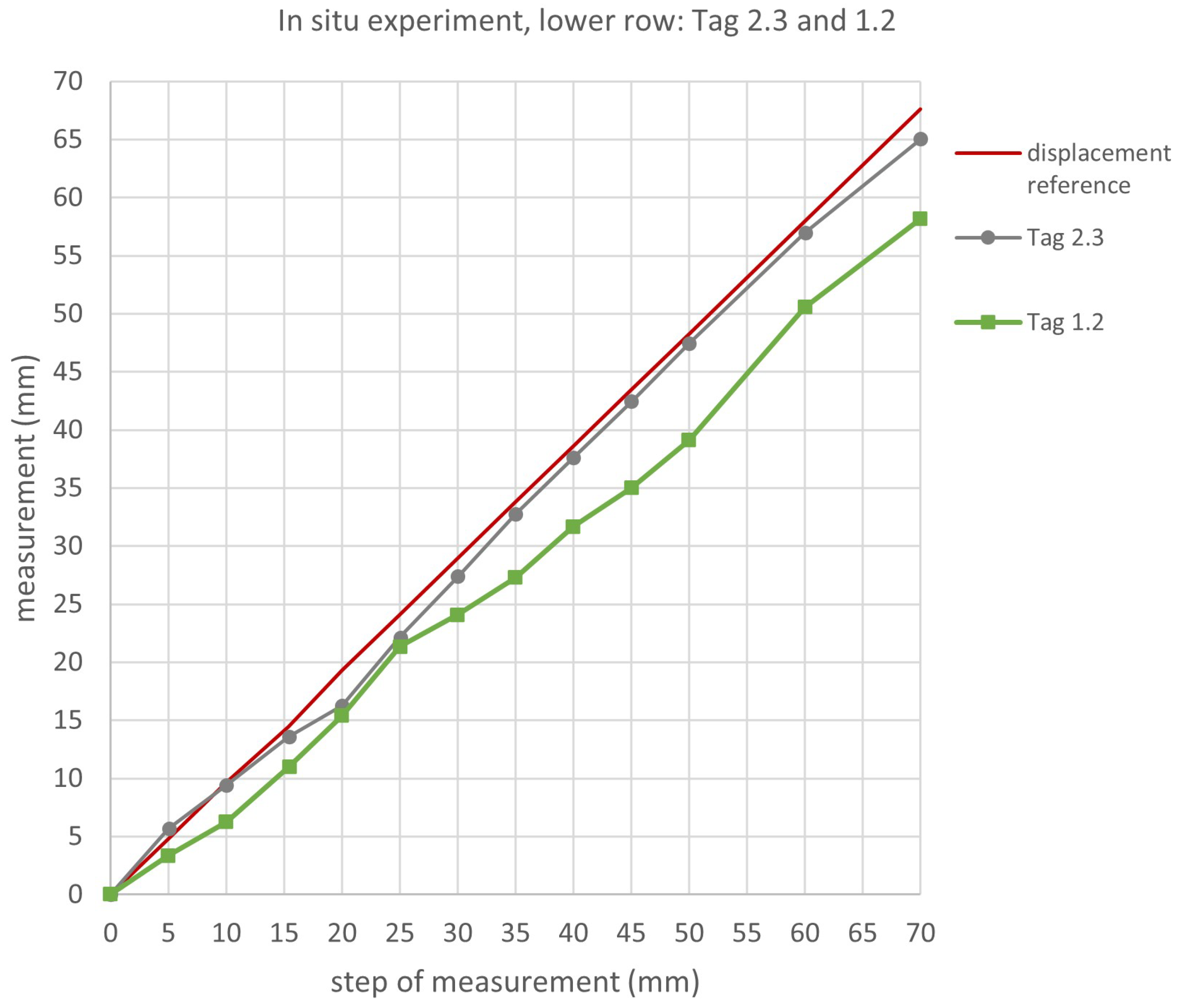
4.2. Test on the 2nd Wall: Comparison between Wireless Tags Displacements and Displacements of the Wired Transducer

In regards to the test performed on the 2nd wall, the results of the signal acquisition of Tag 2.4, Tag 2.2, Tag 2.1, Tag 1.4, Tag 2.3, and Tag 1.2 are reported in Figure 39, Figure 40, Figure 41, Figure 42, Figure 43, and Figure 44, respectively. The values of the mean and standard deviation of the recorded phase for each step of measurement, and RSSI values, are reported for each tag.
As can be observed from the graphs, the values of the phase are increasing at each measurement step, from 0 mm to the maximum displacement of 70 mm (see from Figure 39, Figure 40, Figure 41, Figure 42, Figure 43 and Figure 44). Also, in this case, the t is sensitive to the displacements that occur on the wall.
The distance differences have been calculated according to Equation (1).
The displacements of the tags in the out-of-plane direction, have been geometrically calculated as for the previous tests. The following graphs compare the displacements of the tags in the out-of-plane direction and the displacements detected by the transducer. Also, in this case, the measurements to consider as reference for the tags positioned up and below the middle of the wall were calculated considering a theoretic model, and were plotted together with the results of the tags as reference for comparison.
The displacements detected by Tag 2.4 and 2.2 are reported in Figure 45 compared with the calculated displacements of the wired transducer (plotted as displacement reference). The displacements detected by central row Tags 2.1 and 1.4 are reported in Figure 46 and the displacements of the lower row Tags 2.3 and 1.2 are reported in Figure 47.
As shown in the graphs of Figure 45, Figure 46 and Figure 47, the displacements detected by the t in the in situ test are lower than those recorded simultaneously by the wired transducer. Substantially, the same hypotheses made for the test on the 1st wall can be advanced.
Since the power of the acquisition system and the layout of the tags have remained the same for the in situ test, (compared to the laboratory test with the same tags), the causes of a lower response are due to the environmental conditions of the experimental set-up.
The steel frame used to mount the load cell and constrain the wall and the metal walls of the building, all contribute to negatively affect the performance of the tags, giving smaller displacements compared to the actual ones.
In particular, the tags that were placed on the left side (Tag 2.4 and 2.1) showed smaller displacements, except for Tag 2.3.
Tag 2.3 in fact is the only Tag that correctly matches the actual displacements.
The tags positioned on the right side are less affected by the presence of the metal, in particular Tag 1.4 and 1.2.
In this test, it is observed a generally better response for the lower row t. It is not easy to establish the causes, but it is supposed that the environment and its interference are crucial in determining a good response.

5. Conclusions

The use of commercial passive UHF-RFID tags in the field of civil engineering for monitoring out-of-plane displacements of brick walls has been investigated and discussed. The novelty of this research concerns the application of commercial tags as simple movement sensors. In particular, we used LabID UH105 passive tags, which are tags that are created and used in logistics, etc. The feasibility of the utilization of the tags in the proposed way was assessed by means of laboratory and in situ tests. The set-ups of the in situ tests were organized taking into account the same distances and spaces used in the laboratory tests, in order to compare the results with the same layout conditions, apart from environmental conditions.
Some conclusions can be drawn:
  • The response of the t in the laboratory environment was demonstrated to be very satisfactory, proving that the new application of wireless RFID tags for the monitoring of out-of-plane displacements is feasible and potentially very reliable.
  • A weaker response of some t can be attributed to the intrinsic measurement errors of the reader itself and the errors in processing the received data (standard deviations of the calculated mean values of the phases) and to environmental interference together with the position of the tags with respect to the antenna.
  • In situ experiments showed a weaker response of the t which registered displacements lower than those recorded by the wired transducer used as reference. The high presence of metal in the environment affected negatively the transmission of the electromagnetic signals, modifying the phases and consequently the indirect measurements of displacements. Unluckily, the position of the experimental set-ups necessarily near a metal wall of the building site contributed to negatively affecting the displacement results and the set-ups required steel frames to constrain the single walls and to fix the load cell.
  • Technology limits related to environmental interference can be overcome in future research by using commercial UHF-RFID tags for the real-time monitoring of an existing masonry facade that does not need a steel frame and can potentially respond adequately and properly transmit the electromagnetic signal.
In conclusion, it can be stated that the application of commercial UHF-RFID devices in the civil engineering field is promising and opens up new scenarios for sustainable, wireless, non-invasive, low-cost, and widespread remote monitoring of structures. Despite some technology limits that can be overcome, the results are very satisfactory. In fact, the use of this new measurement technology allows the advantage of sustainable remote and widespread monitoring.

Author Contributions

Conceptualization, A.G., C.C. and E.D.G.; methodology, A.G., C.C., A.D.N., M.M. and E.D.G.; software, C.C. and A.D.N.; validation, C.C.; formal analysis, C.C. and A.D.N.; resources, A.G.; data curation, C.C. and A.D.N.; writing—original draft preparation, C.C.; writing—review and editing, C.C., A.D.N. and M.M.; supervision, A.G. and E.D.G. All authors have read and agreed to the published version of the manuscript.

Funding

This research received no external funding.

Data Availability Statement

Data is contained within the article.

Conflicts of Interest

The authors declare no conflicts of interest.

Abbreviations

The following abbreviations are used in this manuscript:
UHF-RFIDUltra High-Frequency-Radio Frequency Identification
SHMStructural Health Monitoring
WSNsWireless Sensor Networks
ICIntegrated Circuit
PETPolyethylene terephthalate (polyester)
EPCElectronic Product Code
RSSIReceived Signal Strength Indicator

References

  1. Stepinski, T.; Uhl, T.; Staszewski, W. Advanced Structural Damage Detection: From Theory to Engineering Applications; John Wiley & Sons, Inc.: Hoboken, NJ, USA, 2013. [Google Scholar] [CrossRef]
  2. Gomes, G.F.; Mendéz, Y.A.D.; Alexandrino, P.d.S.L.; da Cunha, S.S., Jr.; Ancelotti, A.C., Jr. The use of intelligent computational tools for damage detection and identification with an emphasis on composites—A review. Compos. Struct. 2018, 196, 44–54. [Google Scholar] [CrossRef]
  3. dos Santos, J.A.; Maia, N.; Soares, C.M.; Soares, C.M. Structural damage identification: A survey. Trends Comput. Struct. Technol. 2008, 1, 1–24. [Google Scholar] [CrossRef]
  4. Kong, X.; Cai, C.S.; Hu, J. The state-of-the-art on framework of vibration-based structural damage identification for decision making. Appl. Sci. 2017, 7, 497. [Google Scholar] [CrossRef]
  5. Li, Y. Hypersensitivity of strain-based indicators for structural damage identification: A review. Mech. Syst. Signal Process. 2010, 24, 653–664. [Google Scholar] [CrossRef]
  6. Wang, S.; Xu, M. Modal strain energy-based structural damage identification: A review and comparative study. Struct. Eng. Int. 2019, 29, 234–248. [Google Scholar] [CrossRef]
  7. Alba-Rodríguez, M.D.; Martínez-Rocamora, A.; González-Vallejo, P.; Ferreira-Sánchez, A.; Marrero, M. Building rehabilitation versus demolition and new construction: Economic and environmental assessment. Environ. Impact Assess. Rev. 2017, 66, 115–126. [Google Scholar] [CrossRef]
  8. Munarim, U.; Ghisi, E. Environmental feasibility of heritage buildings rehabilitation. Renew. Sustain. Energy Rev. 2016, 58, 235–249. [Google Scholar] [CrossRef]
  9. Hodge, V.J.; O’Keefe, S.; Weeks, M.; Moulds, A. Wireless sensor networks for condition monitoring in the railway industry: A survey. IEEE Trans. Intell. Transp. Syst. 2014, 16, 1088–1106. [Google Scholar] [CrossRef]
  10. Zhang, R.; Wood, J.; Young, C.; Taylor, A.; Balint, D.; Charalambides, M. A numerical investigation of interfacial and channelling crack growth rates under low-cycle fatigue in bi-layer materials relevant to cultural heritage. J. Cult. Herit. 2021, 49, 70–78. [Google Scholar] [CrossRef]
  11. Li, H.N.; Ren, L.; Jia, Z.G.; Yi, T.H.; Li, D.S. State-of-the-art in structural health monitoring of large and complex civil infrastructures. J. Civ. Struct. Health Monit. 2016, 6, 3–16. [Google Scholar] [CrossRef]
  12. Seo, J.; Hu, J.W.; Lee, J. Summary Review of Structural Health Monitoring Applications for Highway Bridges. J. Perform. Constr. Facil. 2016, 30, 824. [Google Scholar] [CrossRef]
  13. Kulkarni, S.S.; Achenbach, J.D. Structural health monitoring and damage prognosis in fatigue. Struct. Health Monit. 2008, 7, 37–49. [Google Scholar] [CrossRef]
  14. Dissanayake, P.; Karunananda, P. Reliability Index for Structural Health Monitoring of Aging Bridges. Struct. Health Monit. 2008, 7, 175–183. [Google Scholar] [CrossRef]
  15. Rivard, P.; Ballivy, G.; Gravel, C.; Saint-Pierre, F. Monitoring of an hydraulic structure affected by ASR: A case study. Cem. Concr. Res. 2010, 40, 676–680. [Google Scholar] [CrossRef]
  16. Anas, S.; Alam, M.; Shariq, M. Damage response of conventionally reinforced two-way spanning concrete slab under eccentric impacting drop weight loading. Def. Technol. 2023, 19, 12–34. [Google Scholar] [CrossRef]
  17. Anas, S.; Alam, M.; Umair, M. Experimental and numerical investigations on performance of reinforced concrete slabs under explosive-induced air-blast loading: A state-of-the-art review. Structures 2021, 31, 428–461. [Google Scholar] [CrossRef]
  18. Song, G.; Wang, C.; Wang, B. Structural Health Monitoring (SHM) of Civil Structures. Appl. Sci. 2017, 7, 789. [Google Scholar] [CrossRef]
  19. Kaloop, M.R.; Kim, D. GPS-structural health monitoring of a long span bridge using neural network adaptive filter. Surv. Rev. 2014, 46, 7–14. [Google Scholar] [CrossRef]
  20. Guzman-Acevedo, G.M.; Vazquez-Becerra, G.E.; Millan-Almaraz, J.R.; Rodriguez-Lozoya, H.E.; Reyes-Salazar, A.; Gaxiola-Camacho, J.R.; Martinez-Felix, C.A. GPS, Accelerometer, and Smartphone Fused Smart Sensor for SHM on Real-Scale Bridges. Adv. Civ. Eng. 2019, 2019, 15. [Google Scholar] [CrossRef]
  21. Kong, Q.; Allen, R.M.; Kohler, M.D.; Heaton, T.H.; Bunn, J. Structural Health Monitoring of Buildings Using Smartphone Sensors. Seismol. Res. Lett. 2018, 89, 594–602. [Google Scholar] [CrossRef]
  22. Sivasuriyan, A.; Vijayan, D.S.; Górski, W.; Wodzyński, Ł.; Vaverková, M.D.; Koda, E. Practical Implementation of Structural Health Monitoring in Multi-Story Buildings. Buildings 2021, 11, 263. [Google Scholar] [CrossRef]
  23. Lynch, J.P. An overview of wireless structural health monitoring for civil structures. Philos. Trans. R. Soc. Math. Phys. Eng. Sci. 2007, 365, 345–372. [Google Scholar] [CrossRef] [PubMed]
  24. Lynch, J.P.; Loh, K.J. A summary review of wireless sensors and sensor networks for structural health monitoring. Shock Vib. Dig. 2006, 38, 91–130. [Google Scholar] [CrossRef]
  25. Abdulkarem, M.; Samsudin, K.; Rokhani, F.Z.; A Rasid, M.F. Wireless sensor network for structural health monitoring: A contemporary review of technologies, challenges, and future direction. Struct. Health Monit. 2020, 19, 693–735. [Google Scholar] [CrossRef]
  26. Sofi, A.; Regita, J.J.; Rane, B.; Lau, H.H. Structural health monitoring using wireless smart sensor network—An overview. Mech. Syst. Signal Process. 2022, 163, 108113. [Google Scholar] [CrossRef]
  27. Huang, J.; He, L.; Xue, J.; Zhou, S.; Briseghella, B.; Castoro, C.; Aloisio, A.; Marano, G. Dynamic assessment of a stress-ribbon CFST arch bridge with SHM and NDE. In Life-Cycle of Structures and Infrastructure Systems; CRC Press: Boca Raton, FL, USA, 2023; pp. 2762–2769. [Google Scholar]
  28. He, L.; Castoro, C.; Aloisio, A.; Zhang, Z.; Marano, G.C.; Gregori, A.; Deng, C.; Briseghella, B. Dynamic assessment, FE modelling and parametric updating of a butterfly-arch stress-ribbon pedestrian bridge. Struct. Infrastruct. Eng. 2022, 18, 1064–1075. [Google Scholar] [CrossRef]
  29. Aygün, B.; Cagri Gungor, V. Wireless sensor networks for structure health monitoring: Recent advances and future research directions. Sens. Rev. 2011, 31, 261–276. [Google Scholar] [CrossRef]
  30. Ramos, L.F.; Aguilar, R.; Lourenço, P.B.; Moreira, S. Dynamic structural health monitoring of Saint Torcato church. Mech. Syst. Signal Process. 2013, 35, 1–15. [Google Scholar] [CrossRef]
  31. Pallarés, F.J.; Betti, M.; Bartoli, G.; Pallarés, L. Structural health monitoring (SHM) and Nondestructive testing (NDT) of slender masonry structures: A practical review. Constr. Build. Mater. 2021, 297, 123768. [Google Scholar] [CrossRef]
  32. Barsocchi, P.; Bartoli, G.; Betti, M.; Girardi, M.; Mammolito, S.; Pellegrini, D.; Zini, G. Wireless Sensor Networks for Continuous Structural Health Monitoring of Historic Masonry Towers. Int. J. Archit. Herit. 2020, 15, 22–44. [Google Scholar] [CrossRef]
  33. Roy, S.; Jandhyala, V.; Smith, J.R.; Wetherall, D.J.; Otis, B.P.; Chakraborty, R.; Buettner, M.; Yeager, D.J.; Ko, Y.C.; Sample, A.P. RFID: From supply chains to sensor nets. Proc. IEEE 2010, 98, 1583–1592. [Google Scholar] [CrossRef]
  34. Caizzone, S.; DiGiampaolo, E.; Marrocco, G. Wireless crack monitoring by stationary phase measurements from coupled RFID tags. IEEE Trans. Antennas Propag. 2014, 62, 6412–6419. [Google Scholar] [CrossRef]
  35. Caizzone, S.; DiGiampaolo, E. Wireless passive RFID crack width sensor for structural health monitoring. IEEE Sens. J. 2015, 15, 6767–6774. [Google Scholar] [CrossRef]
  36. Caizzone, S.; DiGiampaolo, E.; Marrocco, G. Constrained pole-zero synthesis of phase-oriented RFID sensor antennas. IEEE Trans. Antennas Propag. 2015, 64, 496–503. [Google Scholar] [CrossRef]
  37. DiNatale, A.; DiCarlofelice, A.; DiGiampaolo, E. A Crack Mouth Opening Displacement Gauge Made with Passive UHF RFID Technology. IEEE Sens. J. 2022, 22, 174–181. [Google Scholar] [CrossRef]
  38. Paggi, C.; Occhiuzzi, C.; Marrocco, G. Sub-millimeter displacement sensing by passive UHF RFID antennas. IEEE Trans. Antennas Propag. 2013, 62, 905–912. [Google Scholar] [CrossRef]
  39. DiGiampaolo, E.; DiCarlofelice, A.; Gregori, A. An RFID-Enabled Wireless Strain Gauge Sensor for Static and Dynamic Structural Monitoring. IEEE Sens. J. 2017, 17, 286–294. [Google Scholar] [CrossRef]
  40. Martínez-Martínez, J.J.; Herraiz-Martínez, F.J.; Galindo-Romera, G. A Contactless RFID System Based on Chipless MIW Tags. IEEE Trans. Antennas Propag. 2018, 66, 5064–5071. [Google Scholar] [CrossRef]
  41. Jayawardana, D.; Liyanapathirana, R.; Zhu, X. RFID-Based Wireless Multi-Sensory System for Simultaneous Dynamic Acceleration and Strain Measurements of Civil Infrastructure. IEEE Sens. J. 2019, 19, 12389–12397. [Google Scholar] [CrossRef]
  42. Wang, Q.; Zhang, C.; Ma, Z.; Jiao, G.; Jiang, X.; Ni, Y.; Wang, Y.; Du, Y.; Qu, G.; Huang, J. Towards long-transmission-distance and semi-active wireless strain sensing enabled by dual-interrogation-mode RFID technology. Struct. Control. Health Monit. 2022, 29. [Google Scholar] [CrossRef]
  43. Gregori, A.; DiGiampaolo, E.; DiCarlofelice, A.; Castoro, C. Presenting a New Wireless Strain Method for Structural Monitoring: Experimental Validation. J. Sensors 2019, 2019, 5370838. [Google Scholar] [CrossRef]
  44. Gregori, A.; Castoro, C.; DiNatale, A.; Mercuri, M.; DiGiampaolo, E. Using commercial UHF-RFID wireless tags to detect structural damage. Procedia Struct. Integr. 2023, 44, 1586–1593. [Google Scholar] [CrossRef]
  45. Liu, G.; Wang, Q.A.; Jiao, G.; Dang, P.; Nie, G.; Liu, Z.; Sun, J. Review of Wireless RFID Strain Sensing Technology in Structural Health Monitoring. Sensors 2023, 23, 6925. [Google Scholar] [CrossRef] [PubMed]
  46. Mercuri, M.; Pathirage, M.; Gregori, A.; Cusatis, G. Computational modeling of the out-of-plane behavior of unreinforced irregular masonry. Eng. Struct. 2020, 223, 111181. [Google Scholar] [CrossRef]
  47. Mercuri, M.; Pathirage, M.; Gregori, A.; Cusatis, G. On the collapse of the masonry Medici tower: An integrated discrete-analytical approach. Struct. Eng. Rev. 2021, 246, 113046. [Google Scholar] [CrossRef]
  48. Cecchi, A.; Sab, K. Out of plane model for heterogeneous periodic materials: The case of masonry. Eur. J. -Mech.-A/Solids 2002, 21, 715–746. [Google Scholar] [CrossRef]
  49. Smilović Zulim, M.; Radnić, J. Anisotropy Effect of Masonry on the Behaviour and Bearing Capacity of Masonry Walls. Adv. Mater. Sci. Eng. 2020, 2020, 5676901. [Google Scholar] [CrossRef]
  50. Dominici, D.; Galeota, D.; Gregori, A.; Rosciano, E.; Alicandro, M.; Elaiopoulos, M. Integrating geomatics and structural investigation in post-earthquake monitoring of ancient monumental Buildings. J. Appl. Geod. 2014, 8, 141–154. [Google Scholar] [CrossRef]
  51. Li, X.; Gao, G.; Zhu, H.; Li, Q.; Zhang, N.; Qi, Z. UHF RFID tag antenna based on the DLS-EBG structure for metallic objects. IET Microwaves Antennas Propag. 2020, 14, 567–572. [Google Scholar] [CrossRef]
  52. Moraru, A.; Ursachi, C.; Helerea, E. A New Washable UHF RFID Tag: Design, Fabrication, and Assessment. Sensors 2020, 20, 3451. [Google Scholar] [CrossRef]
  53. Wang, P.; Dong, L.; Wang, H.; Li, G.; Di, Y.; Xie, X.; Huang, D. Passive Wireless Dual-Tag UHF RFID Sensor System for Surface Crack Monitoring. Sensors 2021, 21, 882. [Google Scholar] [CrossRef] [PubMed]
  54. Erman, F.; Koziel, S.; Leifsson, L. Broadband/Dual-Band Metal-Mountable UHF RFID Tag Antennas: A Systematic Review, Taxonomy Analysis, Standards of Seamless RFID System Operation, Supporting IoT Implementations, Recommendations, and Future Directions. IEEE Internet Things J. 2023, 10, 14780–14797. [Google Scholar] [CrossRef]
  55. Zhu, X.; Mukhopadhyay, S.K.; Kurata, H. A review of RFID technology and its managerial applications in different industries. J. Eng. Technol. Manag. 2012, 29, 152–167. [Google Scholar] [CrossRef]
  56. Nambiar, A.N. RFID technology: A review of its applications. In Proceedings of the World Congress on Engineering and Computer Science, San Francisco, CA, USA, 20–22 October 2009; International Association of Engineers: Hong Kong, China, 2009; Volume 2, pp. 20–22. [Google Scholar]
  57. Kumar, P.; Reinitz, H.; Simunovic, J.; Sandeep, K.; Franzon, P. Overview of RFID technology and its applications in the food industry. J. Food Sci. 2009, 74, R101–R106. [Google Scholar] [CrossRef]
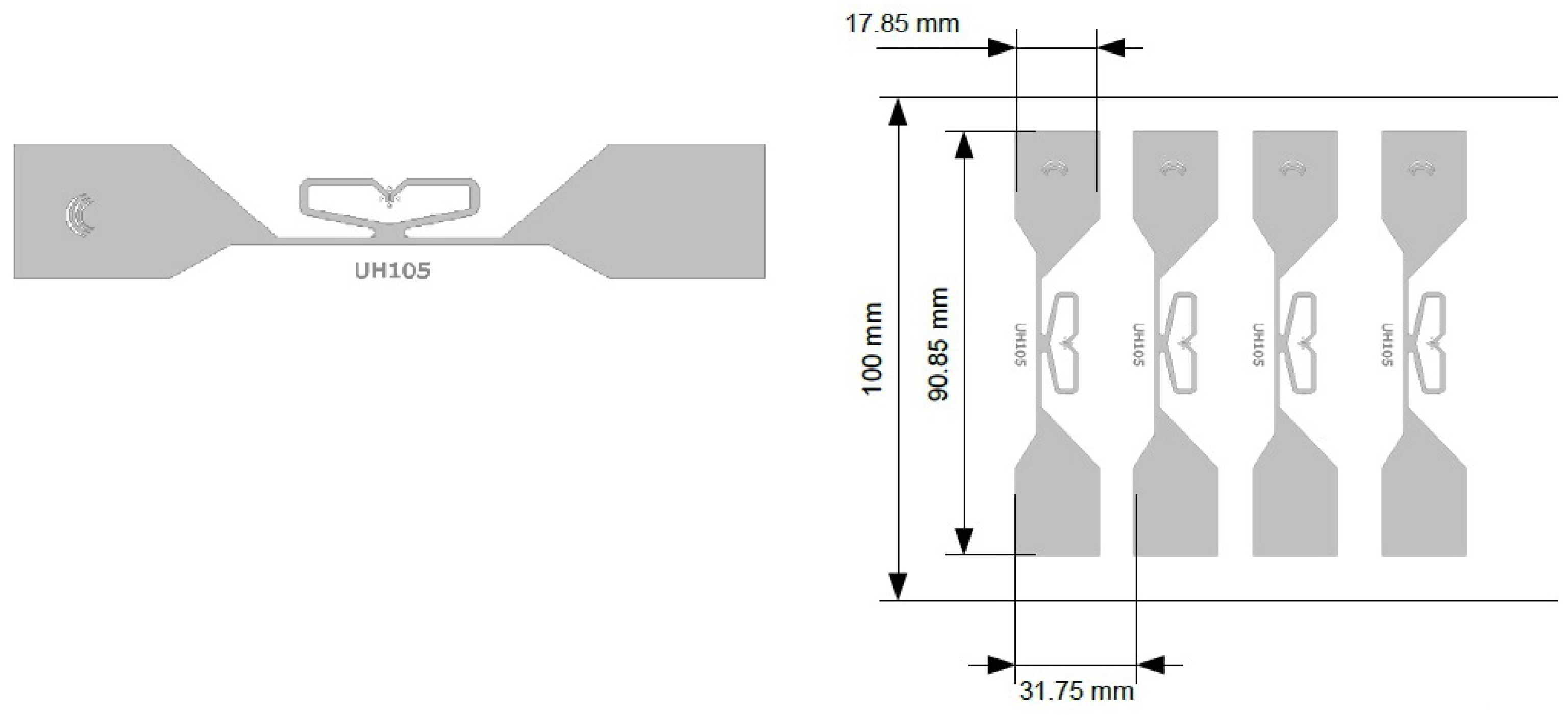
Figure 1. Example of an RFID reading system and its components: Tag, Antenna, Reader, Computer.
Buildings 14 01155 g001
Figure 2. A detail of the commercial UH105 passive tag.
Buildings 14 01155 g002
Figure 3. Radiation pattern of the commercial UH105 passive tag.
Buildings 14 01155 g003
Figure 4. Scheme of the experimental set-up of the 1st laboratory test.
Buildings 14 01155 g004
Figure 5. Scheme of the experimental set-up of the 2nd laboratory test.
Buildings 14 01155 g005
Figure 6. 2nd laboratory campaign: experimental set-up.
Buildings 14 01155 g006
Figure 7. 1st laboratory test: mean and standard deviation of phase (left side ) and RSSI (right side) recorded for each step of measurement of Tag 1.4.
Buildings 14 01155 g007
Figure 8. 1st laboratory test: mean and standard deviation of phase (left side) and RSSI (right side) recorded for each step of measurement of Tag 2.1.
Buildings 14 01155 g008
Figure 9. 1st laboratory test: mean and standard deviation of phase (left side) and RSSI (right side) recorded for each step of measurement of Tag 1.3.
Buildings 14 01155 g009
Figure 10. 1st laboratory test: mean and standard deviation of phase (left side) and RSSI (right side) recorded for each step of measurement of Tag 1.1.
Buildings 14 01155 g010
Figure 11. 1st laboratory test: mean and standard deviation of phase (left side) and RSSI (right side) recorded for each step of measurement of Tag 1.5.
Buildings 14 01155 g011
Figure 12. 1st laboratory test: mean and standard deviation of phase (left side) and RSSI (right side) recorded for each step of measurement of Tag 2.2.
Buildings 14 01155 g012
Figure 13. Flowchart of the methodology used to obtain the results.
Buildings 14 01155 g013
Figure 14. 1st laboratory test: Upper row Tag 1.4 and 2.1. Comparison between the displacements measured using tags and that imposed on the panel (displacement reference).
Buildings 14 01155 g014
Figure 15. First laboratory test: Central row Tag 1.3 and 1.1. Comparison between the displacements measured using tags and that imposed on the panel (displacement reference).
Buildings 14 01155 g015
Figure 16. First laboratory test: Lower row Tag 1.5 and 2.2. Comparison between the displacements measured using tags and that imposed on the panel (displacement reference).
Buildings 14 01155 g016
Figure 17. 2nd laboratory test: mean and standard deviation of phase (left side) and RSSI (right side) recorded for each step of measurement for Tag 2.4.
Buildings 14 01155 g017
Figure 18. 2nd laboratory test: mean and standard deviation of phase (left side) and RSSI (right side) recorded for each step of measurement for Tag 2.2.
Buildings 14 01155 g018
Figure 19. 2nd laboratory test: mean and standard deviation of phase (left side) and RSSI (right side) recorded for each step of measurement for Tag 2.1.
Buildings 14 01155 g019
Figure 20. 2ond laboratory test: mean and standard deviation of phase (left side) and RSSI (right side) recorded for each step of measurement for Tag 1.4.
Buildings 14 01155 g020
Figure 21. 2nd laboratory test: mean and standard deviation of phase (left side) and RSSI (right side) recorded for each step of measurement for Tag 2.3.
Buildings 14 01155 g021
Figure 22. 2nd laboratory test: mean and standard deviation of phase (left side) and RSSI (right side) recorded for each step of measurement for Tag 1.2.
Buildings 14 01155 g022
Figure 23. 2nd laboratory test: Upper row Tag 2.4 and 2.2. Comparison of displacements detected by the tags with that imposed on the panel (displacement reference).
Buildings 14 01155 g023
Figure 24. 2nd laboratory test: Central row Tag 2.1 and 1.4. Comparison of displacements detected by the tags with that imposed on the panel (displacement reference).
Buildings 14 01155 g024
Figure 25. 2nd laboratory test: Lower row Tag 2.3 and 1.2. Comparison of displacements detected by the tags with that imposed on the panel (displacement reference).
Buildings 14 01155 g025
Figure 26. Scheme of the in-situ experimental set-up of the first wall.
Buildings 14 01155 g026
Figure 27. Scheme of the in-situ experimental set-up of the second wall.
Buildings 14 01155 g027
Figure 28. In situ experimental test conducted on the 1st wall: (1 ) Set-up; (2) first deformations and cracks; (3) Maximum deformation reached at 60 mm of displacement.
Buildings 14 01155 g028
Figure 29. In situ experimental test conducted on the 2nd wall: (1) Set-up; (2) Complete deformation of the wall in correspondence of the final displacement of 70 mm.
Buildings 14 01155 g029
Figure 30. In situ experimental test on the 1st wall: mean and standard deviation of phase (left side) and RSSI (right side) recorded for each step of measurement of Tag 1.4.
Buildings 14 01155 g030
Figure 31. In situ experimental test on the 1st wall: mean and standard deviation of phase (left side) and RSSI (right side) recorded for each step of measurement of Tag 2.1.
Buildings 14 01155 g031
Figure 32. In situ experimental test on the 1st wall: mean and standard deviation of phase (left side) and RSSI (right side) recorded for each step of measurement of Tag 1.3.
Buildings 14 01155 g032
Figure 33. In situ experimental test on the 1st wall: mean and standard deviation of phase (left side) and RSSI (right side) recorded for each step of measurement of Tag 1.1.
Buildings 14 01155 g033
Figure 34. In situ experimental test on the 1st wall: mean and standard deviation of phase (left side) and RSSI (right side) recorded for each step of measurement of Tag 1.5.
Buildings 14 01155 g034
Figure 35. In situ experimental test on the 1st wall: mean and standard deviation of phase (left side) and RSSI (right side) recorded for each step of measurement of Tag 2.2.
Buildings 14 01155 g035
Figure 36. In situ experimental test on the 1st wall: the displacements detected by Tags 2.1 and 1.4 are compared with the calculated displacements of the wired transducer.
Buildings 14 01155 g036
Figure 37. In situ experimental test on the 1st wall: the displacements detected by Tags 1.1 and 1.3 are compared with the calculated displacements of the wired transducer.
Buildings 14 01155 g037
Figure 38. In situ experimental test on the 1st wall: the displacements detected by Tags 2.2 and 1.5 are compared with the calculated displacements of the wired transducer.
Buildings 14 01155 g038
Figure 39. In situ experimental test on the 2nd wall: mean and standard deviation of phase (left side) and RSSI (right side) recorded for each step of measurement of Tag 2.4.
Buildings 14 01155 g039
Figure 40. In situ experimental test on the 2nd wall: mean and standard deviation of phase (left side) and RSSI (right side) recorded for each step of measurement of Tag 2.2.
Buildings 14 01155 g040
Figure 41. In situ experimental test on the 2nd wall: mean and standard deviation of phase (left side) and RSSI (right side) recorded for each step of measurement of Tag 2.1.
Buildings 14 01155 g041
Figure 42. In situ experimental test on the 2nd wall: mean and standard deviation of phase (left side) and RSSI (right side) recorded for each step of measurement of Tag 1.4.
Buildings 14 01155 g042
Figure 43. In situ experimental test on the 2nd wall: mean and standard deviation of phase (left side) and RSSI (right side) recorded for each step of measurement of Tag 2.3.
Buildings 14 01155 g043
Figure 44. In situ experimental test on the 2nd wall: mean and standard deviation of phase (left side) and RSSI (right side) recorded for each step of measurement of Tag 1.2.
Buildings 14 01155 g044
Figure 45. In situ experimental test on the 2nd wall: the displacements detected by the upper row Tags 2.4 and 2.2 are compared to the calculated displacements detected by the wired transducer.
Buildings 14 01155 g045
Figure 46. In situ experimental test on the 2nd wall: the displacements detected by Tags 2.1 and 1.4 are compared with the calculated displacements of the wired transducer.
Buildings 14 01155 g046
Figure 47. In situ experimental test on the 2nd wall: the displacements detected by Tags 2.3 and 1.2 are compared with the calculated displacements of the wired transducer.
Buildings 14 01155 g047
Table 1. Characteristics of the tag UH105.
CompositionMaterialThickness [μm]
TopAluminum9 ± 5%
SupportPolyester PET38 ± 5%
TagOperating frequencyOperating temperature
840–960 MHz−40 °C to +85 °C
Disclaimer/Publisher’s Note: The statements, opinions and data contained in all publications are solely those of the individual author(s) and contributor(s) and not of MDPI and/or the editor(s). MDPI and/or the editor(s) disclaim responsibility for any injury to people or property resulting from any ideas, methods, instructions or products referred to in the content.

