
A Review of Static and Dynamic p-y Curve Models for Pile Foundations


Abstract
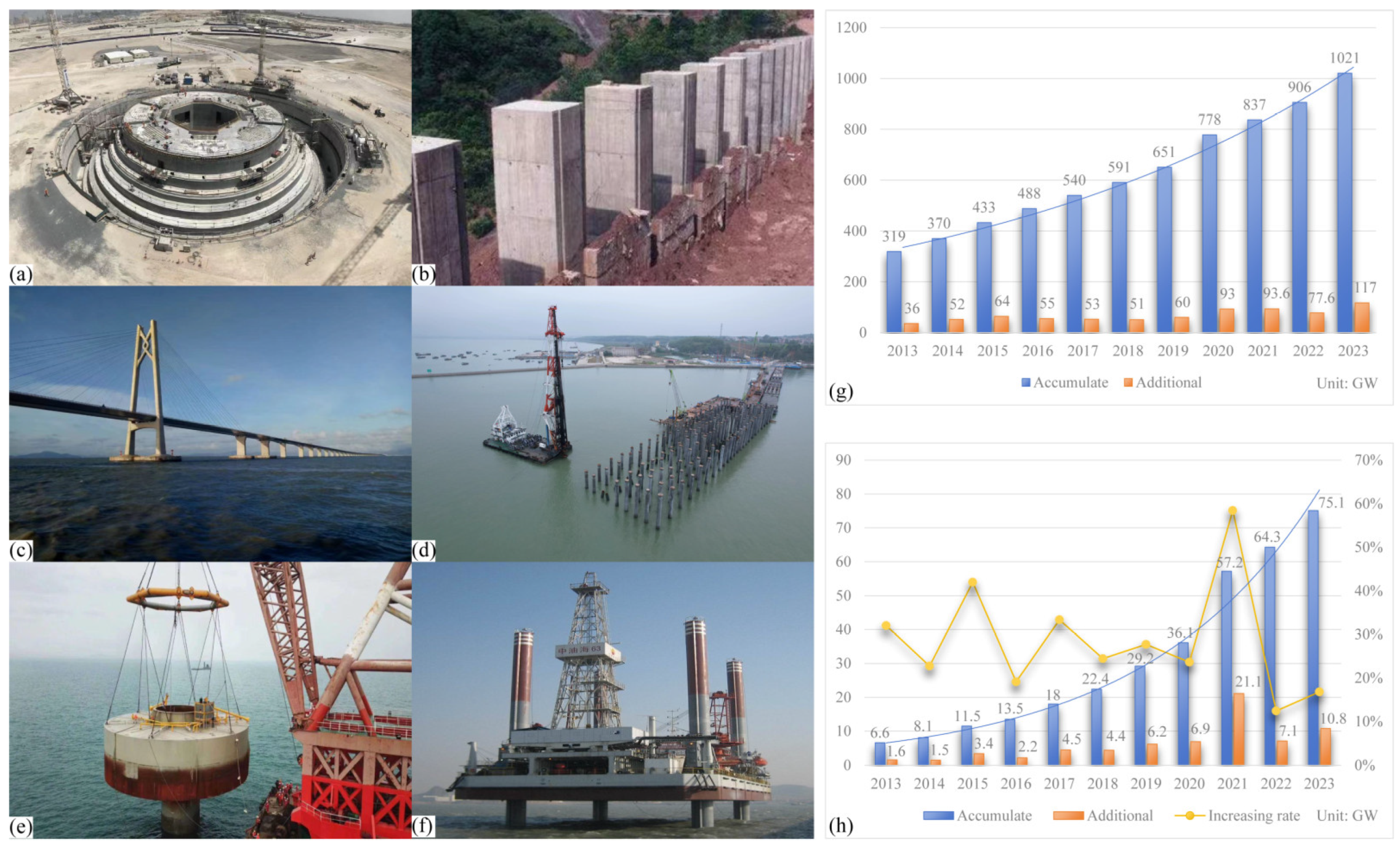
1. Introduction
2. Static p-y Curve Model
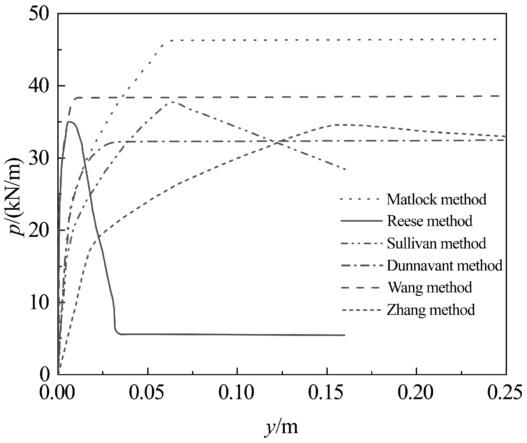
2.1. Static p-y Curves for Clay


| References | p-y Curve Model | Model Description |
|---|---|---|
| Matlock (1970) [5] | Divided into two segments with 8 as the boundary, applicable to soft clay | |
| Reese (1975) [7] | Applicable to underwater stiff clay | |
| Dunnavant and O’Neill (1989) [15] | Based on full-scale pile load tests | |
| Wang (1991) [16] | are all parameters | |
| Zhang (1992) [18] | Piecewise function with the critical depth as the boundary | |
| Zhou (2013) [20] | Applicable to soft clay | |
| Chen (2018) [25] | Piecewise function for large-diameter winged piles in soft clay | |
| Zhang (2020) [11] | Based on the stress increment theory, errors exist under small displacements in sand | |
| Zhang (2020) [23] | Applicable to large-diameter single piles |
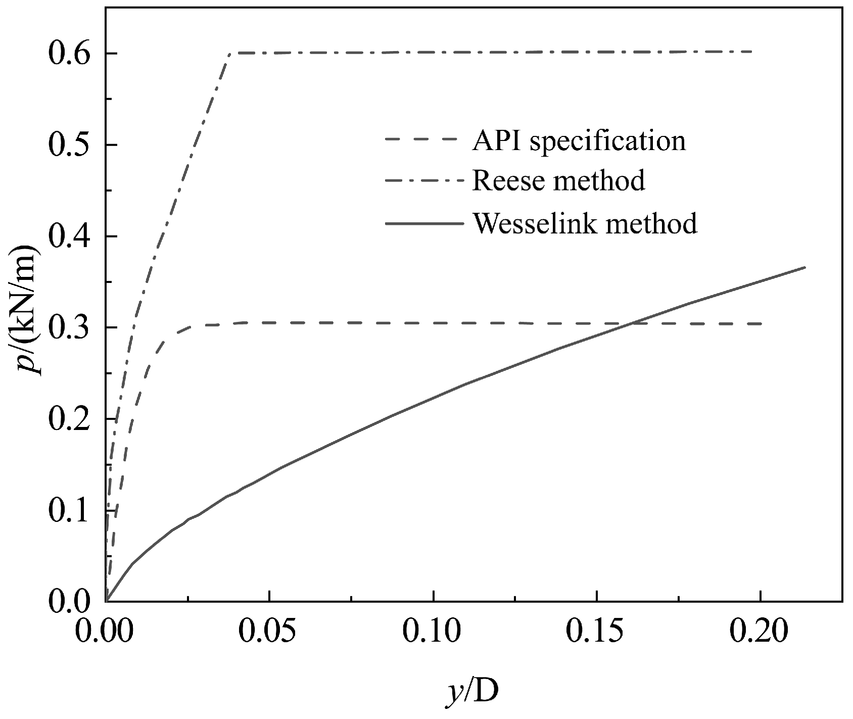
2.2. Static p-y Curves for Sand
2.2.1. API Specification Type p-y Curve
2.2.2. Hyperbolic-Shaped p-y Curve
2.2.3. Discussion on Sand p-y Curves
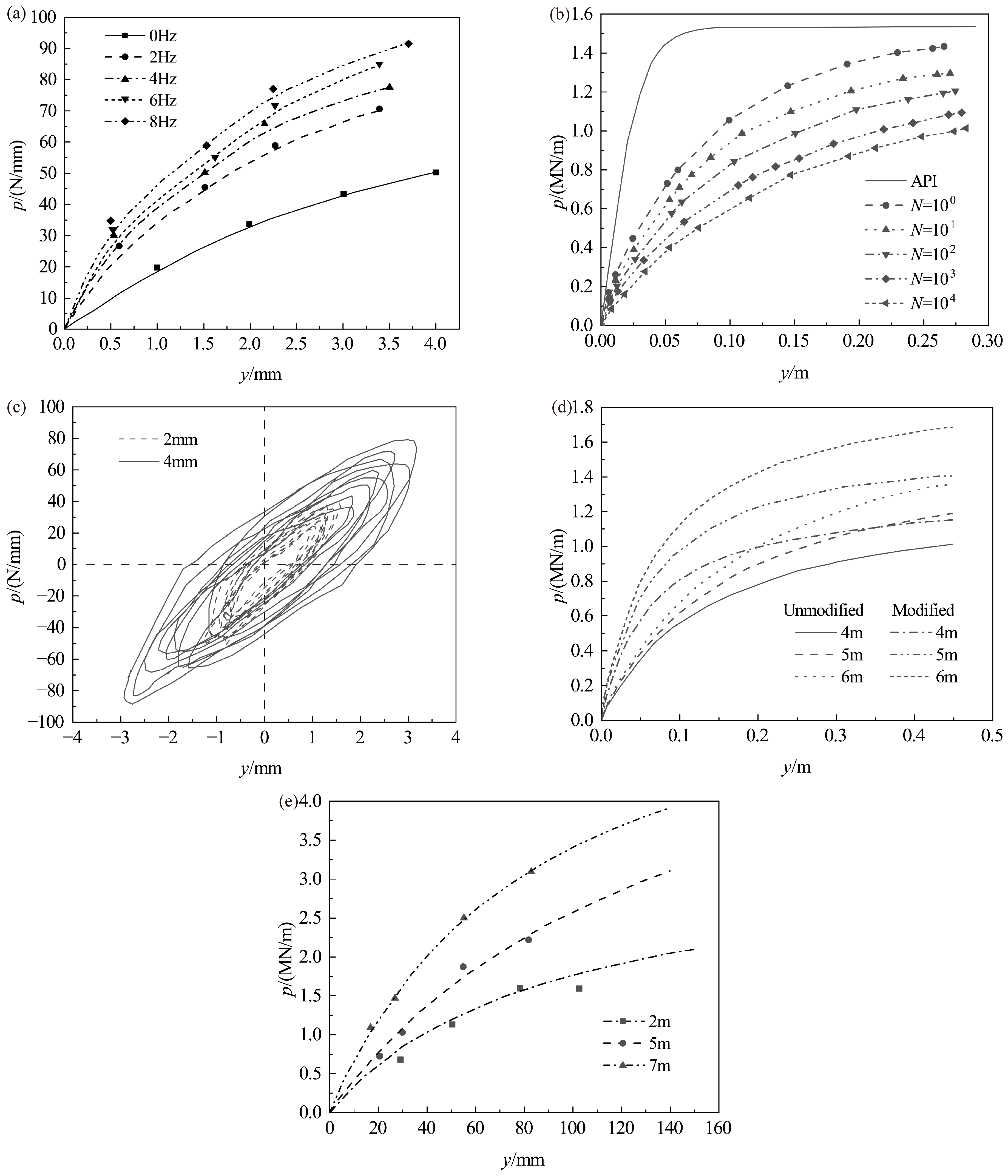
3. Cyclic p-y Curves
3.1. Cyclic p-y Curve Models
3.1.1. Reduction Coefficient Method
3.1.2. Empirical Fitting Method
3.1.3. Unified Method
3.1.4. Normalization Method
3.2. Analysis of Influencing Factors
4. Seismic p-y Curves
4.1. Seismic p-y Curve Models
4.1.1. p-Multiplier Method
4.1.2. Empirical Fitting Method
4.1.3. Other Methods
4.2. Discussion on Seismic p-y Curve Models
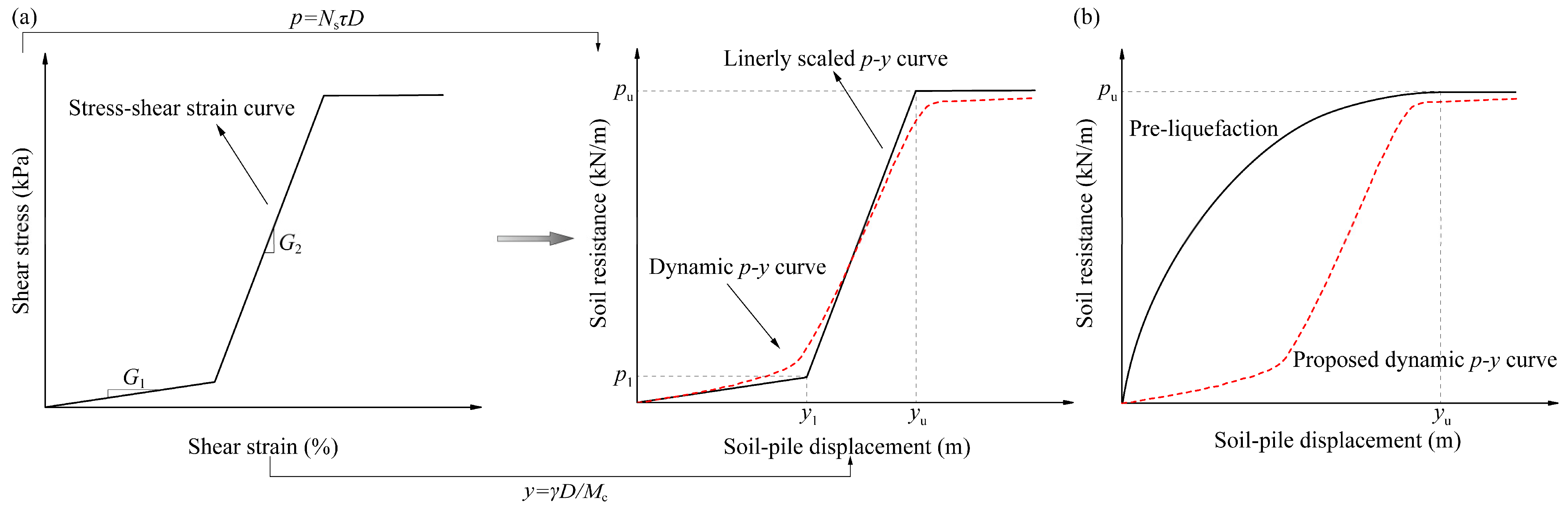
4.2.1. Shape of Seismically Liquefied Soil p-y Curves
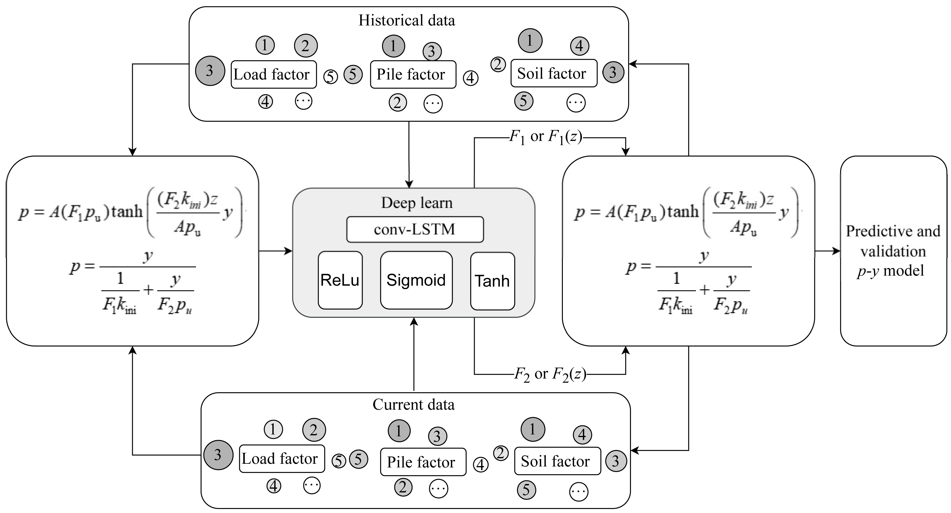
4.2.2. Discussion on the p-Multiplier Method
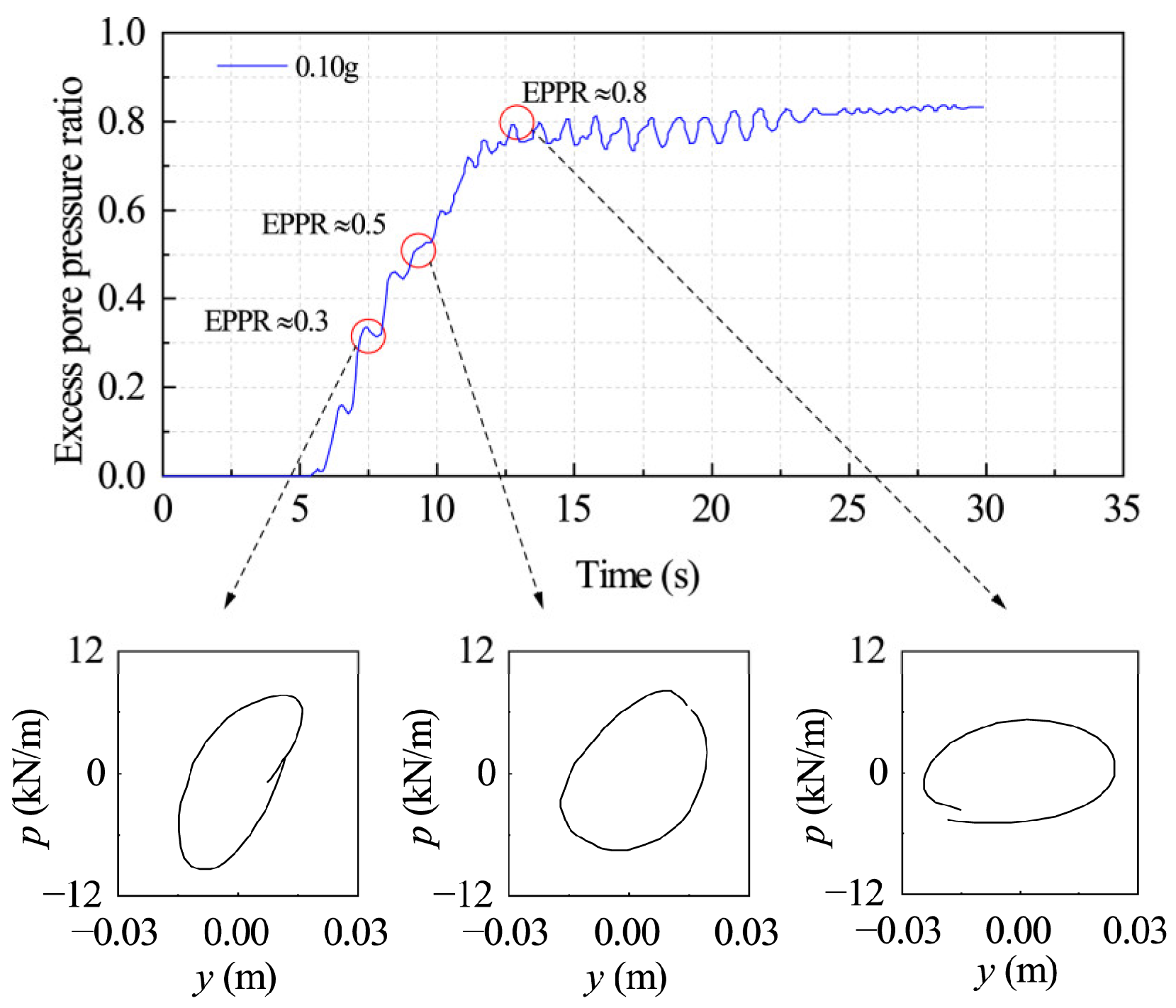
4.2.3. Factors Influencing Seismic p-y Curves
5. Discussion
6. Conclusions
Author Contributions
Funding
Data Availability Statement
Conflicts of Interest
References
- JGJ 94-2008; Technical Specifications for Construction Pile Foundations. Ministry of Housing and Urban-Rural Development of the People’s Republic of China: Beijing, China, 2008.
- Bai, X.Y.; He, Q.; Zhao, Y. Discussion of m-method and p-y curve method in pile foundation calculation for bridges on soft soil sites. Transp. Sci. Technol. 2019, 5, 64–68. [Google Scholar]
- RP2GEO; Geotechnical Consideration and Foundation Design for Offshore Structures. American Petroleum Institute: Houston, TX, USA, 2014.
- JTG 3363-2019; Highway Bridge Foundation and Foundation Design Specification. Ministry of Transport of the People’s Republic of China: Beijing, China, 2019.
- Matlock, H. Correlation for design of laterally loaded piles in soft clay. In Proceedings of the Offshore Technology Conference, Houston, TX, USA, 21–23 April 1970. [Google Scholar]
- Reese, L.C.; Cox, W.R.; Koop, F.D. Analysis of laterally loaded piles in sand. In Proceedings of the 6th Annual Offshore Technology Conference, Houston, TX, USA, 5–7 May 1974. [Google Scholar]
- Reese, L.C.; Welch, R.C. Lateral loading of deep foundations in stiff clay. J. Geo. Eng. Div. 1975, 101, 633–649. [Google Scholar] [CrossRef]
- Sun, B.W.; Jiang, C.; Pang, L.; Liu, P.; Li, X.T. Effect of the pile diameter and slope on the undrained lateral response of the Large-Diameter pile. Comput. Geotech. 2022, 152, 104981. [Google Scholar] [CrossRef]
- Wang, W.; Yan, J.Y.; Liu, J.P.; Yu, G.M.; Zhang, Z.C. Study on combination of p-y models for laterally loaded pile in offshore wind farm. Ocean Eng. 2022, 265, 112640. [Google Scholar] [CrossRef]
- Kim, J.; Kim, G.; Lee, J. Dynamic p-y analysis method based on cone penetration test results for monopiles in sand. Soil Dyn. Earthq. Eng. 2022, 163, 107503. [Google Scholar] [CrossRef]
- Zhang, X.L.; Zhao, J.J.; Xu, C.S. A method for p-y curve based on Vesic expansion theory. Soil Dyn. Earthq. Eng. 2020, 137, 106291. [Google Scholar]
- Ghazavi, M.; Mahmoodi, E.; El Naggar, H. Load-deflection analysis of laterally loaded piles in unsaturated soils. Acta Geotech. 2023, 18, 2217–2238. [Google Scholar] [CrossRef]
- Lee, P.Y.; Gilbert, L.W. Behavior of laterally loaded pile in very soft clay. In Proceedings of the Offshore Technology Conference, Houston, TX, USA, 30 April–3 May 1979. [Google Scholar]
- Sullivan, W.R.; Reese, L.C.; Fenske, C.W. Unified Method for Analysis of Laterally Loaded Piles in Clay; Institution of Civil Engineers, Numerical in Offshore Piling: London, UK, 1980. [Google Scholar]
- Dnnavant, T.W.; O’Neill, M.W. Experimental p-y model for submerged stiff clay. J. Geotech. Eng. 1989, 115, 95–114. [Google Scholar] [CrossRef]
- Wang, H.C.; Wu, D.Q.; Tian, P. A new unified method for transverse static load pile p-y curves in clay coils. J. Hohai Univ. 1991, 19, 9–17. [Google Scholar]
- Tian, P.; Wang, H.C. Unified method of p-y curve for transverse periodically loaded piles in clay soils. J. Hohai Univ. 1993, 21, 9–14. [Google Scholar]
- Zhang, L.Y.; Chen, Z.C. A method for calculating p-y curves of cohesive soils. Ocean Eng. 1992, 10, 50–58. [Google Scholar]
- Wang, G.C.; Yang, M. Calculation method of horizontally loaded pile foundation in clay soil. J. Tongji Univ. 2012, 40, 373–378. [Google Scholar]
- Zhou, T.Q.; Lu, Z.A.; Wang, D.H. Calculation method for laterally loaded ultra-long PHC piles. Port Waterw. Eng. 2013, 6, 155–160. [Google Scholar]
- Zeng, S.P.; Ye, G.L.; Chen, J.J. Numerical analysis of horizontal loading on single piles with p-y curves in clay. Spec. Struct. 2016, 33, 94–98. [Google Scholar]
- Wang, A.H.; Zhang, D.W.; Xie, J.C. Study on horizontal bearing characteristics of rigid composite piles in soft clay using p-y curves. Chin. J. Geotech. Eng. 2020, 42, 381–389. [Google Scholar]
- Zhang, H.Y.; Liu, R.; Yuan, Y.; Liang, C. Correction of p-y curve for large diameter monopile foundation in the sea. J. Hydraul. Eng. 2020, 51, 201–211. [Google Scholar]
- Hu, Y.Z.; Lu, Z.A.; Zhai, Q.; Zhang, Y.Q. Exploration of p-y curves of Large Diameter Plus-Wing Piles in Soft Clay Soils. Water Resour. Hydropower Eng. 2018, 49, 143–152. [Google Scholar]
- Chen, C.M.; Su, X.D.; He, J.X.; Wang, X.P.; Huang, W.L. Study on the horizontal bearing performance of large-diameter plus-wing piles for offshore wind power. Ocean Eng. 2018, 36, 97–104,146. [Google Scholar]
- Jiao, Y.Q.; Qiao, D.S.; Wang, B.; Tang, G.Q.; Lu, L.; Ou, J.P. Three-spring soil reaction model for wind turbine monopile foundation in clay. Appl. Ocean Res. 2024, 144, 103911. [Google Scholar] [CrossRef]
- Scott, R.F. Analysis of Centrifuge Pile Tests: Simulation of Pile Driving; American Petroleum Institute: Pasadena, CA, USA, 1980. [Google Scholar]
- Murchison, J.M.; O’Neill, M.W. Evaluation of p-y relationships in cohesionless soils. In Analysis and Design of Pile Foundations; Power Research Institute: New York, NY, USA, 1984. [Google Scholar]
- Zhou, J.W. Comparative analysis of two p-y curve methods for sandy soils. Build. Struct. 2019, 49, 837–840. [Google Scholar]
- Kondner, R.L. Hyperbolic stress-strain response: Cohesive soils. J. Soil Mech. 1963, 89, 115–143. [Google Scholar] [CrossRef]
- Kim, B.T.; Kim, N.K.; Lee, W.J.; Kim, Y.S. Experimental load-transfer curves of laterally loaded piles in Nak-Dong river sand. J. Geotech. Geoenviron. 2004, 130, 416–425. [Google Scholar]
- Lim, H.; Jeong, S. Simplified p-y curves under dynamic loading in dry sand. Soil Dyn. Earthq. Eng. 2018, 113, 101–111. [Google Scholar] [CrossRef]
- Yang, E.K.; Choi, J.I.; Kwon, S.Y.; Kim, M.M. Development of dynamic p-y backbone curves for a single pile in dense sand by 1g shaking table tests. KSCE J. Civ. Eng. 2011, 15, 813–821. [Google Scholar] [CrossRef]
- Wesselink, B.D.; Murff, J.D.; Randolph, M.F.; Nunez, I.L.; Hyden, A.M. Analysis of centrifuge model test data from laterally loaded piles in calcareous sand. In Engineering for Calcareous Sediments, 1st ed.; Andrews, D., Jewell, R., Eds.; CRC Press: Rotterdam, The Netherlands, 1988; Volume 1, pp. 261–270. [Google Scholar]
- Wang, G.C.; Yang, M. Nonlinear analysis of piles under horizontal loading in sandy soil. Rock Soil Mech. 2011, 32, 261–267. [Google Scholar]
- Hu, Z.B.; Zhai, E.D.; Luo, L.B.; Yang, X.G. Research on sandy soil p-y curves for offshore wind turbine monopiles based on static loading tests. Acta Energiae Solaris Sin. 2019, 40, 3571–3577. [Google Scholar]
- Sun, Y.L.; Xu, C.S.; Du, X.L.; Du, X.P.; Xi, R.Q. Modified p-y curve model for large diameter monopiles in offshore wind power. Eng. Mech. 2021, 38, 44–53. [Google Scholar] [CrossRef]
- Cao, W.P.; Xia, B.; Ge, X. Development and application of hyperbolic p-y curves for laterally loaded batter piles. J. Zhejiang Univ. (Eng. Sci.) 2019, 53, 1946–1954. [Google Scholar]
- Ling, D.S.; Ren, T.; Wang, Y.G. Horizontal bearing characteristics of inclined piles for sandy soil foundations by p-y curve method. Rock Soil Mech. 2013, 34, 155–162. [Google Scholar]
- Fu, C.; Zhuang, Y.Z.; Chen, B.C.; Fan, Z.H. Analysis on p-y curves of micro-pile in sand. Chin. J. Undergr. Space Eng. 2017, 13, 1271–1279. [Google Scholar]
- Sun, X.; Huang, W.P. Study on the p-y curve of large-diameter piles for offshore wind power based on field measurement data. Acta Energiae Solaris Sin. 2016, 37, 216–221. [Google Scholar]
- Zhang, X.L.; Zhou, R.; Zhang, G.L.; Han, Y. A corrected p-y curve model for large-diameter pile foundation of offshore wind turbine. Ocean Eng. 2023, 273, 114012. [Google Scholar] [CrossRef]
- Wang, T.; Wang, T.L. Experimental research on silt p-y curves. Rock. Soil Mech. 2009, 30, 1343–1346. [Google Scholar]
- Liu, H.J.; Lv, X.H.; Zhang, D.D.; Wang, Z.L. Experimental study of p-y curves of lateral loaded single-piles in the Yellow River Delta silt. Ind. Constr. 2014, 44, 79–83. [Google Scholar]
- Zhang, M.; Huang, J.Z.; Wang, Y.; Gong, W.M.; Dai, G.L. Model test study on p-y curve of silt. Build. Struct. 2022, 52, 2456–2462. [Google Scholar]
- Gao, M.; Chen, J.Z.; Zheng, G.F.; Fang, H.L. Study on behavior of lateral loaded piles under static, dynamic and cyclic loadings and proposal of p-y curve formulation. Ocean Eng. 1988, 6, 34–44. [Google Scholar]
- Wang, Z.Y.; Liu, H.J.; Hu, R.G. The review of p-y curve model for lateral cyclic loaded pile. Mar. Sci. Bull. 2020, 39, 401–407. [Google Scholar]
- Gerolymos, N.; Escoffier, S.; Gaztas, G.; Garnier, J. Numerical modeling of centrifuge cyclic lateral pile load experiments. Earthq. Eng. Eng. Vib. 2009, 8, 61–76. [Google Scholar] [CrossRef]
- Bienen, B.; Dührkop, J.; Grabe, J.; Randolph, M.F.; White, D.J. Response of piles with wings to monotonic and cyclic lateral loading in sand. J. Geotech. Geoenviron. 2012, 138, 364–375. [Google Scholar] [CrossRef]
- Zhu, B.; Xiong, G.; Liu, J.C.; Sun, Y.X.; Chen, R.P. Centrifuge modelling of a large-diameter single pile under lateral loads in sand. Chin. J. Geotech. Eng. 2013, 35, 1807–1815. [Google Scholar]
- Liu, H.J.; Zhang, D.D.; Lv, X.H.; Wang, H. Experimental study on horizontal bearing characteristics of saturated powder foundation monopile under cyclic loading. Period. Ocean Univ. China (Nat. Sci.) 2015, 45, 76–82. [Google Scholar]
- Zhong, C.; Mao, D.F.; Ni, M.C.; Huang, J.; Yan, C.; Li, X.H.; Zhang, T. Research on pile-soil interaction considering the degradation of pile foundation. China Offshore Oil Gas 2015, 27, 98–104, 110. [Google Scholar]
- Baek, S.H.; Kim, J.Y.; Lee, S.H.; Chung, C.K. Development of the cyclic p-y curve for a single pile in sandy soil. Mar. Georesources Geotechnol. 2017, 36, 351–359. [Google Scholar] [CrossRef]
- Lee, M.; Bae, K.T.; Lee, I.W.; Yoo, M. Cyclic p-y curves of monopiles in dense dry sand using centrifuge mode tests. Appl. Sci. 2019, 9, 1641. [Google Scholar] [CrossRef]
- Broms, B.B. Lateral resistance of piles in cohesionless soils. J. Soil Mech. Found. Div. 1964, 90, 123–158. [Google Scholar] [CrossRef]
- Hu, A.F.; Nan, B.W.; Chen, Y.; Fu, P. Modified p-y curves method based on degradation stiffness model of sand. J. Shanghai Jiaotong Univ. 2020, 54, 1316–1323. [Google Scholar]
- Fuentes, W.; Gil, M.; Rivillas, G. A p-y model for large diameter monopiles in sands subjected to lateral loading under static and long-term cyclic conditions. J. Geotech. Geoenviron. Eng. 2021, 147, 04020164. [Google Scholar] [CrossRef]
- Chen, X.L.; Guan, C.Y.; Zhang, G.W.; Dai, G.L.; Gao, L.C.; Wan, Z.H. Simplified p-y curves for horizontally loaded monopiles of offshore wind turbines. Acta Energiae Solaris Sin. 2022, 43, 366–371. [Google Scholar]
- Zhang, F.; Liu, J.B.; Wu, J.B. The study on single pile model test in soft clay under cyclic lateral loading. Sichuan Build. Sci. 2017, 43, 56–60. [Google Scholar]
- Wu, Y.J.; Lu, C.Y.; Li, W.C.; Yang, M. A modified p-y curve model applied to the characterization of horizontally loaded piles in marine engineering. J. Dalian Univ. Technol. 2018, 58, 511–518. [Google Scholar]
- Sun, Y.X.; Liu, H.T.; He, C.H.; Zhu, Y.; Zhu, B. Research on pile-soil interaction of a rigid pile subjected to cyclic loading in silt foundation. Ind. Constr. 2018, 48, 111–115, 181. [Google Scholar]
- Zhang, L.Y.; Chen, Z.C. Response characteristics of monopiles in cohesive soils under lateral cyclic loading. China Harb. Eng. 1990, 000, 7–12. [Google Scholar]
- Wang, H.; Wang, L.Z.; Hong, Y.; Masin, D.; Li, W.; He, B.; Pan, H.L. Centrifuge testing on monotonic and cyclic lateral behavior of large-diameter slender piles in sand. Ocean Eng. 2021, 226, 108299. [Google Scholar] [CrossRef]
- Zhang, L.Y.; Silva, F.; Grismala, R. Ultimate lateral resistance to piles in cohesionless soils. J. Geotech. Geoenviron. Eng. 2005, 131, 78–83. [Google Scholar] [CrossRef]
- Barton, Y.O. Laterally Loaded Model Piles in Sand: Centrifuge Tests and Finite Element Analyses. Ph.D. Thesis, University of Cambridge, Cambridge, UK, 1982. [Google Scholar]
- Kim, G.; Kyung, D.; Park, D.; Lee, J. CPT-based p-y analysis for mono-piles in sands under static and cyclic loading conditions. Geomech. Eng. 2015, 9, 313–328. [Google Scholar] [CrossRef]
- Kim, G.; Kyung, D.; Park, D.; Kim, I.; Lee, J. CPT-Based p-y analysis for piles embedded in clays under cyclic loading conditions. KSCE J. Civ. Eng. 2016, 20, 1759–1768. [Google Scholar] [CrossRef]
- Liang, F.Y.; Qin, C.R.; Chen, S.Q.; Zhang, H. Model test for dynamic p-y backbone curves of soil-pile interaction under cyclic lateral loading. China Harb. Eng. 2017, 37, 21–26. [Google Scholar]
- Zhu, B.; Ren, J.; Wu, L.Y.; Kong, D.Q.; Ye, G.L.; Tang, Q.J.; Lai, Y. Effect of loading rate on lateral pile-soil interaction in sand considering partially drained condition. China Ocean Eng. 2020, 34, 772–783. [Google Scholar] [CrossRef]
- Nikitas, G.; Arany, L.; Aligaran, S.; Vimalan, J.N.; Bhattacharya, S. Predicting long term performance of offshore wind turbines using cyclic simple shear apparatus. Soil Dyn. Earthq. Eng. 2017, 92, 678–683. [Google Scholar] [CrossRef]
- Yang, G.P.; Zhang, Z.M. Research on p-y curve of laterally bearing piles under large displacement. Port Waterw. Eng. 2002, 342, 40–45+71. [Google Scholar]
- Kong, D.Q.; Wen, K.; Zhu, B.; Zhu, Z.J.; Chen, Y.M. Centrifuge modeling of cyclic lateral behaviors of a tetrapod piled jacket foundation for offshore wind turbines in sand. J. Geotech. Geoenviron. Eng. 2019, 145, 04019099. [Google Scholar] [CrossRef]
- Hong, Y.; Yao, M.H.; Wang, L.Z. A multi-axial bounding surface p-y model with application in analyzing pile responses under multi-directional lateral cycling. Comput. Geotech. 2023, 157, 105301. [Google Scholar] [CrossRef]
- Leblanc, C.; Houlsby, G.T.; Byrne, B.W. Response of stiff piles in sand to long-term cyclic lateral loading. Geotechnique. 2010, 60, 79–90. [Google Scholar] [CrossRef]
- Yang, H.X.; Chen, X.D.; Qi, L. Analysis of mechanical response of monopiles in saturated clay foundations under cyclic loading. Eng. Frontiers. 2020, 5, 9–10+15. [Google Scholar]
- Fu, Z.A.; Wang, G.S.; Yu, Y.M.; Shi, L. Model test study on bearing capacity and deformation characteristics of symmetric pile-bucket foundation subjected to cyclic horizontal load. Symmetry 2021, 13, 1647. [Google Scholar] [CrossRef]
- Zhu, N.; Cui, L.; Liu, J.W.; Wang, M.M.; Zhao, H.; Jia, N. Discrete element simulation on the behavior of open-ended pipe pile under cyclic lateral loading. Soil Dyn. Earthq. Eng. 2021, 144, 106646. [Google Scholar] [CrossRef]
- Heidari, M.; El Naggar, H.; Jahanandish, M.; Ghahramani, A. Generalized cyclic p-y curve modeling for analysis of laterally loaded piles. Soil Dyn. Earthq. Eng. 2014, 63, 138–149. [Google Scholar] [CrossRef]
- Naggar, M.H.E.; Bentley, K.J. Dynamic analysis for laterally loaded piles and dynamic p-y curves. Can. Geotech. J. 2000, 37, 1166–1183. [Google Scholar] [CrossRef]
- Zhu, B.T. Ultimate Resistance of Soils and Laterally Loaded Pile Properties. Ph.D. Thesis, Tongji University, Shanghai, China, 2005. [Google Scholar]
- Liu, L.; Dobry, R. Effect of Liquefaction on Lateral Response of Piles by Centrifuge Model Tests; Bureau of Transportation Statistics: New York, NY, USA, 1995.
- Boulanger, R.W.; Wilson, D.W.; Kutter, B.L.; Abghari, A. Soil-pile-superstructure interaction in liquefiable sand. Transp. Res. Rec. 1997, 1569, 55–64. [Google Scholar] [CrossRef]
- Wang, J.H.; Feng, S.L. Analysis of horizontal bearing characteristics of pile foundations in liquefied soils. Rock Soil Mech. 2005, 26, 76–80. [Google Scholar]
- Gerber, T.M. p-y Curves for Liquefied Sand Subject to Cyclic Loading Based on Testing of Full-Scale Deep Foundations. Ph.D. Thesis, Brigham Young University, Provo, UT, USA, 2003. [Google Scholar]
- Rollins, K.M.; Gerber, T.M.; Lane, J.D.; Ashford, S. Lateral resistance of a full-scale pile group in liquefied sand. J. Geotech. Geoenviron. Eng. 2005, 131, 115–125. [Google Scholar] [CrossRef]
- Chang, B.J.; Hutchinson, T.C. Experimental evaluation of p-y curves considering development of liquefaction. J. Geotech. Geoenviron. Eng. 2013, 139, 577–586. [Google Scholar] [CrossRef]
- Zhang, X.L.; Zu, D.Z.; Xu, C.S.; Du, X.L. Research on p-y curves of soil-pile interaction in saturated sand foundation in weakened state. Rock Soil Mech. 2020, 41, 2252–2260. [Google Scholar]
- Li, Y.R.; Yuan, X.M.; Liang, Y. Modified calculation method of p-y curves for liquefied soil-pile interaction. Chin. J. Geotech. Eng. 2009, 31, 595–599. [Google Scholar]
- Yoo, M.T.; Choi, J.I.; Han, J.T.; Kim, M.M. Dynamic p-y curves for dry sand from centrifuge tests. J. Earthq. Eng. 2013, 17, 1082–1102. [Google Scholar] [CrossRef]
- Yoo, M.; Kwon, S.Y.; Kim, J.Y.; Lee, M.; Jung, S. Development of dynamic p-y curves for piles in soft clay by using 1-g shaking table test. J. Struct. Integr. Maint. 2019, 4, 207–215. [Google Scholar]
- Franke, K.W.; Rollins, K.M. Simplified hybrid p-y spring model for liquefied soils. J. Geotech. Geoenviron. Eng. 2013, 139, 564–576. [Google Scholar] [CrossRef]
- Ling, X.C.; Tang, L. Recent advance of p-y curve to model lateral response of pile foundation on liquefied ground. Advances in Mechanics. 2010, 40, 250–262. [Google Scholar]
- Zhang, Z.; Tang, L.; Ling, X.C.; Si, P.; Tian, S.; Cong, S.Y. p-y curve characteristics of dynamic pile-soil interaction during sand liquefaction. J. Harbin Eng. Univ. 2022, 43, 1433–1439. [Google Scholar]
- Dash, S.R.; Rouholamin, M.; Lombardi, D.; Bhattacharya, S. A practical method for construction of p-y curves for liquefiable soils. J. Soil Dyn. Earthq. Eng. 2017, 97, 478–481. [Google Scholar] [CrossRef]
- Wilson, D.W.; Boulanger, R.W.; Kutter, B.L. Observed seismic lateral resistance of liquefying sand. J. Geotech. Geoenviron. Eng. 2000, 126, 898–906. [Google Scholar] [CrossRef]
- Park, J.S.; Jeong, S.S. Estimation of lateral dynamic p-multiplier of group pile using dynamic numerical analysis results. J. Civ. Environ. Eng. Res. 2018, 38, 567–578. [Google Scholar]
- Lombardi, D.; Bhattacharya, S. Evaluation of seismic performance of pile-supported models in liquefiable soils. Earthq. Eng. Struct D. 2016, 45, 1019–1038. [Google Scholar] [CrossRef]
- Cubrinovski, M.; Kokusho, T.; Ishihara, K. Interpretation from large-scale shake table tests on piles undergoing lateral spreading in liquefied soils. Soil Dyn. Earthq. Eng. 2006, 26, 275–286. [Google Scholar] [CrossRef]
- Choi, J.I.; Kim, M.M.; Brandenberg, S.J. Cyclic p-y plasticity model applied to pile foundations in sand. J. Geotech. Geoenviron. Eng. 2015, 141, 04015013. [Google Scholar] [CrossRef]
- Zhang, J.; Li, Y.R.; Rong, X.; Liang, Y. Dynamic p-y curves for vertical and batter pile groups in liquefied sand. Earthq. Eng. Eng. Vibr. 2022, 21, 605–616. [Google Scholar] [CrossRef]
- Zhang, X.L.; Zhang, B.J.; Zhang, W.X.; Han, Y. Research on dynamic p-y curves in liquefied sand under cyclic loading conditions. Ocean Eng. 2023, 285, 115360. [Google Scholar] [CrossRef]
- Wang, C.Y.; Ding, X.M.; Cao, G.W.; Jian, C.Y.; Fang, H.Q. Numerical investigation of the effect of particle gradation on the lateral response of pile in coral sand. Comput. Geotech. 2022, 152, 316–326. [Google Scholar] [CrossRef]
- McCarron, W.O. Bounding surface model for soil resistance to cyclic lateral pile displacements with arbitrary direction. Comput. Geotech. 2016, 71, 47–55. [Google Scholar] [CrossRef]
- Mu, L.L.; Chen, W.; Zhan, Y.M.; Chen, X.X.; Li, W. A framework of analytical methods for horizontal behaviours of monopiles under V-H-M loads in sand. Mar. Georesources Geotechnol. 2021, 40, 349–360. [Google Scholar] [CrossRef]
- Zhang, Z.C.; Zhang, J.; Wu, X.F.; Wang, Y.B. Quantitative analysis and modification of dynamic p-y curve model for offshore wind turbines considering earthquake history effect based on deep learning. Ocean Eng. 2024, 299, 117372. [Google Scholar] [CrossRef]


| References | p-y Curve Model | Model Description |
|---|---|---|
| Reese (1974) [6] | Based on full-scale experiments | |
| Scott (1980) [27] | Developed based on centrifuge experiments | |
| Murchison and O’Neill (1984) [28] | is the pile type factor, and is the load empirical factor | |
| Gao (1988) [46] | is the correction factor, based on sand model experiments | |
| Kim (2004) [31] | and consider the influence of installation methods and pile head constraint conditions | |
| Wang (2009) [43] | Modified according to API specifications for application in silty soil | |
| Wang (2011) [35] | considers the influence of the pile diameter and is calculated at the soil parameter selection location | |
| Sun (2021) [37] | Stiffness correction based on API, considering pile diameter and depth | |
| Zhang (2022) [45] | Modified according to API specifications for application in silty soil | |
| Zhang (2023) [42] | Modified according to API specifications, applicable to large-diameter single pile in sand |
| References | p-y Curve Model | Model Description |
|---|---|---|
| Gerolymos et al. (2009) [48] | Correction for the influence of soil strength and stiffness parameters | |
| Bienen et al. (2012) [49] | is a correction factor and represents the load conditions | |
| Zhu et al. (2013) [50] | Considering cyclic impact factors | |
| Liu et al. (2015) [51] | in segments based on critical depth (for silty soil) | |
| Zhong et al. (2015) [52] | is the reduction coefficient | |
| Baek et al. (2017) [53] | Considering the influence of relative density and depth | |
| Lee et al. (2019) [54] | calculated based on Broms [55] | |
| Hu et al. (2020) [56] | is the stiffness reduction factor, considers the influence of pile diameter | |
| Fuentes et al. (2021) [57] | Based on API |
Disclaimer/Publisher’s Note: The statements, opinions and data contained in all publications are solely those of the individual author(s) and contributor(s) and not of MDPI and/or the editor(s). MDPI and/or the editor(s) disclaim responsibility for any injury to people or property resulting from any ideas, methods, instructions or products referred to in the content. |
© 2024 by the authors. Licensee MDPI, Basel, Switzerland. This article is an open access article distributed under the terms and conditions of the Creative Commons Attribution (CC BY) license (https://creativecommons.org/licenses/by/4.0/).
Share and Cite
Wu, J.; Pu, L.; Zhai, C. A Review of Static and Dynamic p-y Curve Models for Pile Foundations. Buildings 2024, 14, 1507. https://doi.org/10.3390/buildings14061507
Wu J, Pu L, Zhai C. A Review of Static and Dynamic p-y Curve Models for Pile Foundations. Buildings. 2024; 14(6):1507. https://doi.org/10.3390/buildings14061507
Chicago/Turabian StyleWu, Jiujiang, Longjun Pu, and Changming Zhai. 2024. "A Review of Static and Dynamic p-y Curve Models for Pile Foundations" Buildings 14, no. 6: 1507. https://doi.org/10.3390/buildings14061507
APA StyleWu, J., Pu, L., & Zhai, C. (2024). A Review of Static and Dynamic p-y Curve Models for Pile Foundations. Buildings, 14(6), 1507. https://doi.org/10.3390/buildings14061507