


Finite Element Method Simulation and Experimental Investigation on the Temperature Control System with Groundwater Circulation in Bridge Deck Pavement


Abstract
:1. Introduction
2. Methodology
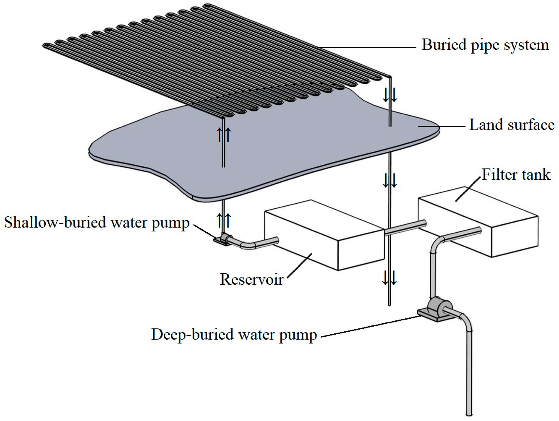
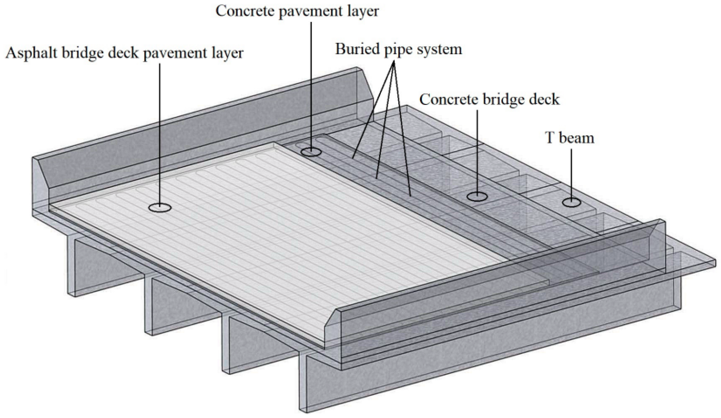
2.1. GCTCS System
2.2. Physics
- The surface water film is evenly distributed, and the film thickness is taken as 3 mm regardless of evaporation and loss.
- The ambient wind speed is in a stable and continuous condition.
- The temperature of the groundwater flow is constant, i.e., the water temperature at the inlet to the input pipe system is maintained.
- The effect of phase-change submersible heat is ignored for the water film.
- The effect of traffic on the road surface is ignored.
- The bridge deck slab connects to the infrastructure through the abutment, and there is thus little thermal conduction.
- The longitudinal axis of the bridge, the bottom area of which is sheltered by the lateral T-beams, is not exposed to solar radiation.
- Wind slows down in the cavity, which reduces heat convection loss (Figure 4 shows the wind speed distribution across the T-beam structure under the action of transverse wind, and the wind speed in the cavity therein is decreased).
2.3. Settings
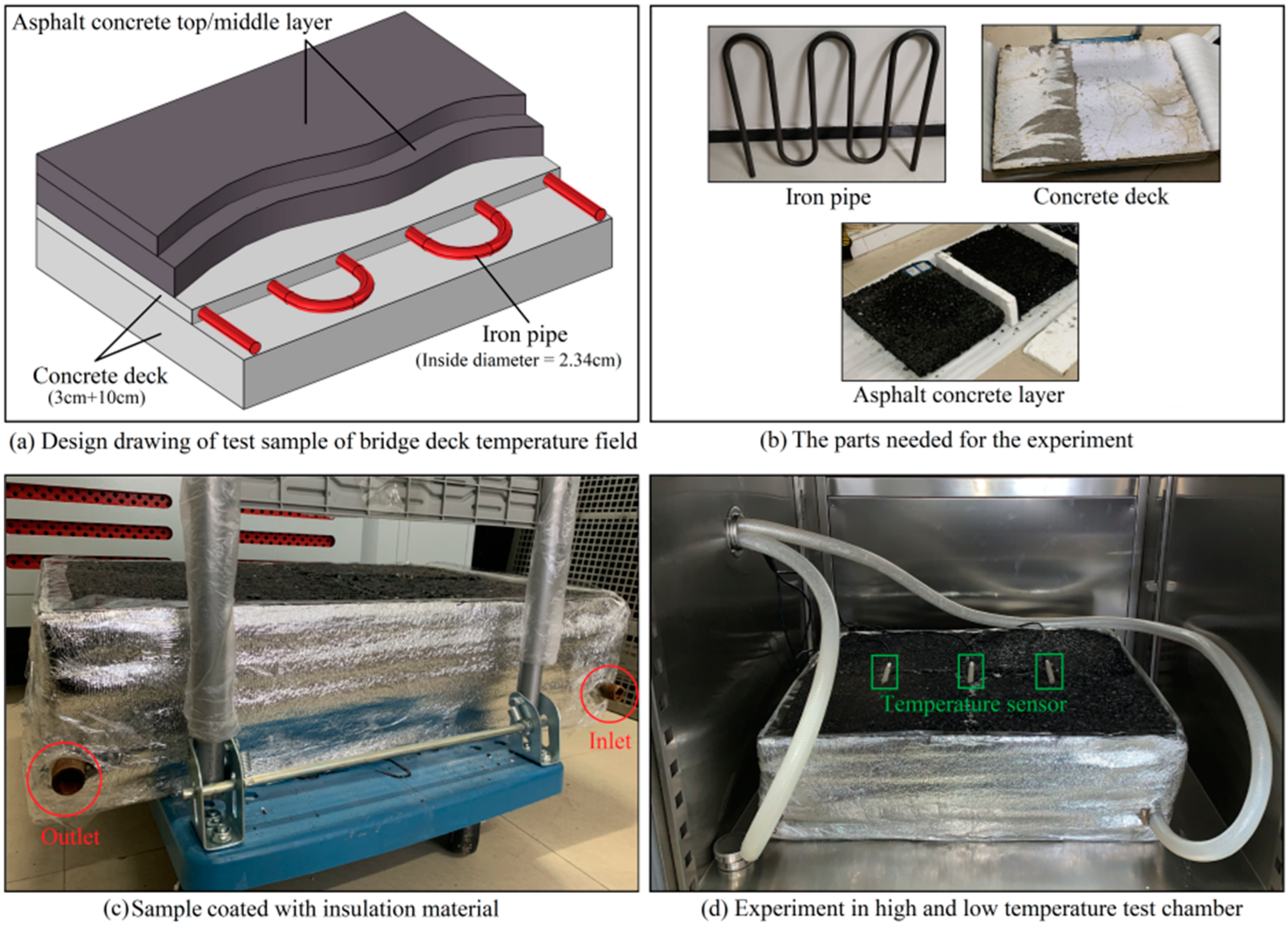
2.4. Experiment
3. Results
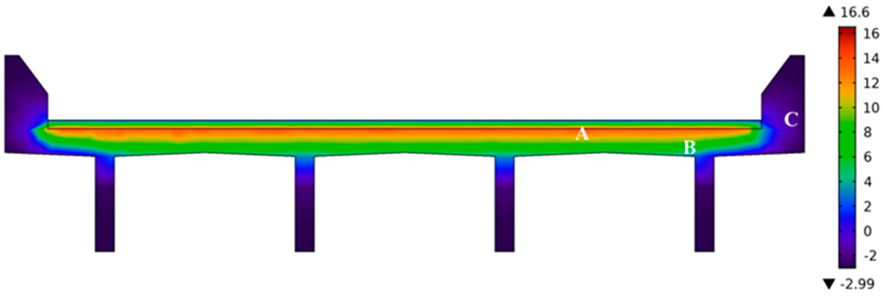
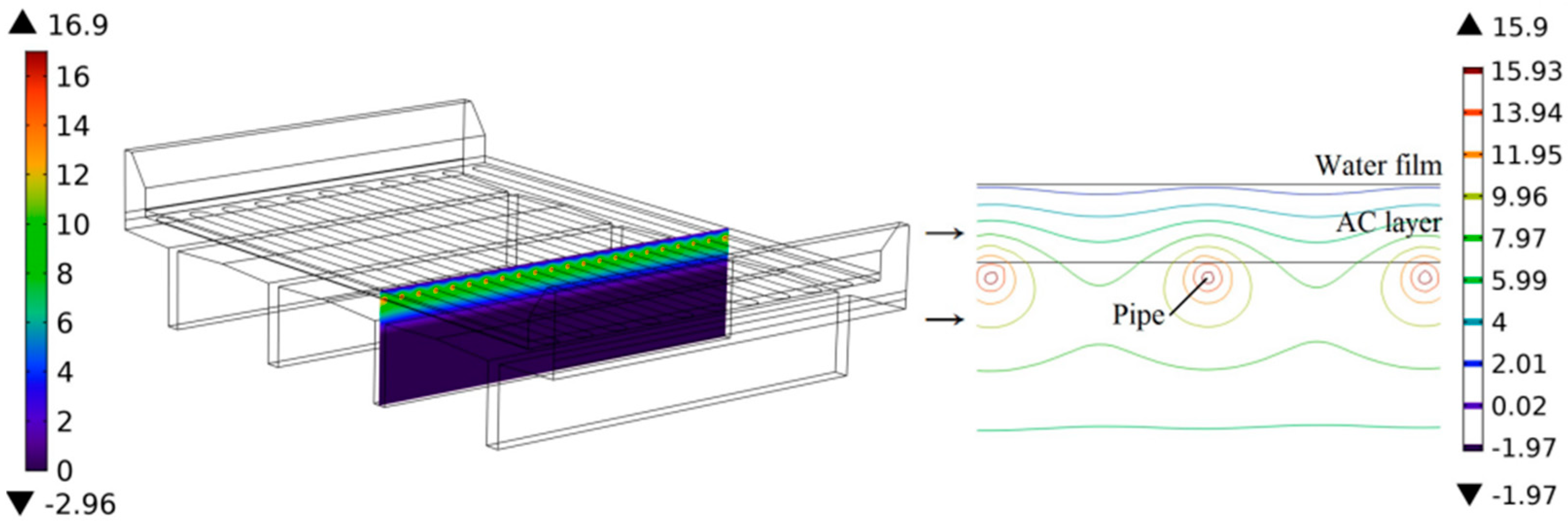
3.1. Steady-State
- Wind speed directly impacts the thermal convection of the surface, leading to a reduction in the temperature of the water film as wind speed increases. However, the cooling effect slows down. The simulation result demonstrates the significant influence of wind speed on the water film temperature (see Figure 8a). For instance, as the wind speed increased from 1.6 m/s to 10.6 m/s, the average water film temperature decreased by 5.6 °C in the simulation. When the wind speed exceeded 10 m/s, the minimum temperature of the water film dropped below 0 °C;
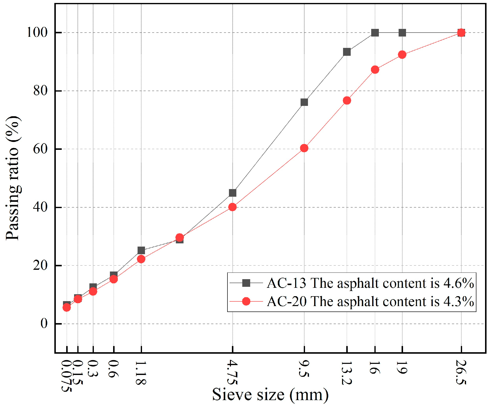
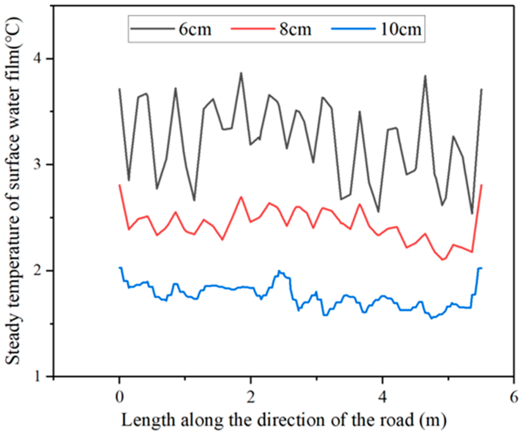
- The variation in the asphalt concrete (AC) layer’s thickness determines the distance between the pipe system and the surface water film, directly affecting the heat transfer. The simulation result indicates that increasing the AC layer thickness leads to a gradual decrease in the water film temperature, along with a reduction in the difference between the maximum and minimum temperatures (see Figure 8b).
- Groundwater temperature plays a crucial role in determining the temperature difference between the interior and exterior of the pipe, thereby affecting heat transfer. Both the simulation and experiment reveal a linear increase in the surface water film temperature with respect to groundwater temperature. When the groundwater temperature reached approximately 13 °C, the minimum temperature remained above the freezing point of water (see Figure 8c).
- The water flow rate determines whether warm water can enter the pipe system in a timely manner for heat release. Increasing the flow rate from 25 L/min to 125 L/min resulted in a relative growth rate of 400%. However, the water film temperature shows a slow increase, with the average temperature rising from 1.65 °C to 2.15 °C in the simulation (see Figure 8d). The experimental results show slightly lower water film temperatures compared to the simulated values, but the overall trend remains the same.
- Pipe spacing governs the temperature field distribution and determines the sufficient flow time for groundwater within the pipe network system. It serves as a comprehensive indicator of system behavior. With an increase in pipe spacing, all four temperature indicators decrease to varying extents, with the minimum temperature exhibiting the most significant reduction, followed by the average temperatures. At a pipe spacing of 100 mm, the temperature difference is only 0.47 °C, whereas at a spacing of 300 mm, the temperature difference rises to 2.65 °C, and the minimum temperature falls below freezing (see Figure 8e).
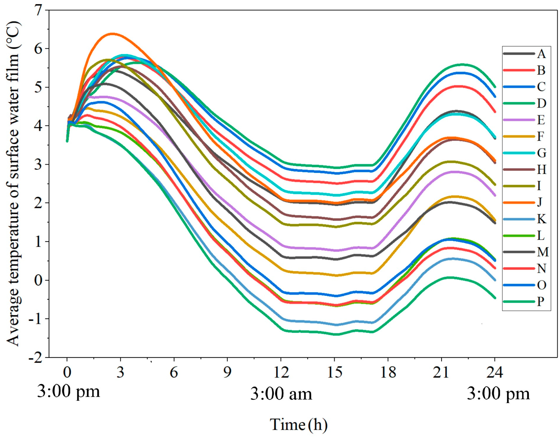
3.2. Transient Effects
4. Discussion
4.1. Wind Speed
4.2. Groundwater Temperature
4.3. Thermal Conductivity
4.4. Pipe Spacing
4.5. AC Layer Thickness and Flow Rate
5. Conclusions
- Wind speed emerges as the most influential factor among the five considered. As wind speed increases, the temperature of the water film experiences a sharp decline. This cooling effect is particularly pronounced at low wind speeds. When the wind speed exceeds 10 m/s, the water film temperature can rapidly drop below the freezing point, with convective heat loss accounting for over 90% of the overall heat loss.
- Groundwater temperature ranks second only to wind speed in terms of its impact on the heat transfer process. A direct linear relationship exists between groundwater temperature and the steady temperature of the water film, with higher groundwater temperatures resulting in higher water film temperatures.
- Pipe spacing noticeably affects the minimum temperature of the surface water film, while the thickness of the AC layer significantly influences the uniformity of the temperature distribution within the water film. Conversely, the flow rate exhibits minimal influence on these factors.
- Enhancing the thermal conductivity of the AC layer and concrete layer proves beneficial in elevating the water film temperature.
Author Contributions
Funding
Data Availability Statement
Conflicts of Interest
References
- Dan, H.C.; He, L.H.; Zou, J.F.; Zhao, L.H.; Bai, S.Y. Laboratory study on the adhesive properties of ice to the asphalt pavement of the highway. Cold Reg. Sci. Technol. 2014, 104, 7–13. [Google Scholar] [CrossRef]
- Hagedorn, R.; Martí-Vargas, J.R.; Dang, C.N.; Hale, W.M.; Floyd, R.W. Temperature gradients in bridge concrete i-girders under a heatwave. J. Bridge Eng. 2019, 24, 04019077. [Google Scholar] [CrossRef]
- Hanbali, R.M. The economic impact of winter road maintenance on road users. Transp. Res. Rec. 1994, 1442, 429–439. [Google Scholar]
- Lund, J.W. Pavement Snow Melting; Geo-Heat Center Quarterly Bull.: Klamath Falls, OR, USA, 2000; Volume 21, pp. 12–19. [Google Scholar]
- Dan, H.C.; Tan, J.W.; Du, Y.F.; Cai, J.M. Simulation and optimization of road de-icing salt usage based on the Water-Ice- Salt Model. Cold Reg. Sci. Technol. 2020, 169, 102917. [Google Scholar] [CrossRef]
- Guo, Q.; Li, G.; Gao, Y.; Wang, K.; Dong, Z.; Liu, F.; Zhu, H. Experimental investigation on bonding property of asphalt-aggregate interface under the actions of salt immersion and freeze-thaw cycles. Constr. Build. Mater. 2019, 206, 590–599. [Google Scholar] [CrossRef]
- Tian, J.; Wu, X.W.; Zheng, Y.; Hu, S.W.; Ren, W.; Du, Y.F.; Wang, W.W.; Sun, C.; Ma, J.; Ye, Y.X. Investigation of damage behaviors of ECC-to-concrete interface and damage prediction model under salt freeze-thaw cycles. Constr. Build. Mater. 2019, 226, 238–249. [Google Scholar] [CrossRef]
- Wright, M.; Parry, T.; Airey, G. Chemical pavement modifications to reduce ice adhesion. Proc. Inst. Civ. Eng.-Transp. 2016, 169, 76–87. [Google Scholar] [CrossRef]
- Gao, J.; Guo, H.; Wang, X.; Wang, P.; Wei, Y.; Wang, Z.; Yang, B. Microwave de-icing for asphalt mixture containing steel wool fibers. J. Clean. Prod. 2019, 206, 1110–1122. [Google Scholar] [CrossRef]
- Du, Y.F.; Wang, J.C.; Deng, H.B.; Liu, Y.C.; Tian, J.; Wu, X.W. Using steel fibers to accelerate the heat conduction in asphalt mixture and its performance evaluation. Constr. Build. Mater. 2021, 282, 122637. [Google Scholar] [CrossRef]
- Wang, Z.; He, Z.; Wang, Z.; Ning, M. Microwave Deicing of Functional Pavement Using Sintered Magnetically Separated Fly Ash as Microwave-Heating Aggregate. J. Mater. Civ. Eng. 2019, 31, 04019127. [Google Scholar] [CrossRef]
- Ho, I.H.; Li, S.; Abudureyimu, S. Alternative hydronic pavement heating system using deep direct use of geothermal hot water. Cold Reg. Sci. Technol. 2019, 160, 194–208. [Google Scholar] [CrossRef]
- Zheng, Q.Q.; Deng, Y.P.; Gan, K. Groundwater and groundwater-source heat pump systems in the urban district of Nanchang. Resour. Surv. Environ. 2010, 31, 66–70. [Google Scholar]
- Hassan, Y.; Abd El Halim, A.O.; Bekheet, W.; Farha, M.H. Effects of runway deicers on pavement materials and mixes: Comparison with road salt. Transp. Eng. 2002, 128, 385–391. [Google Scholar] [CrossRef]
- Abraham, S.P.; Abdelaziz, S.L.; Longtin, J. Heat Exchangers for pavement surface de-icing. Geo-Chicago 2016, 633–643. [Google Scholar]
- Dan, H.C.; He, L.H.; Zhao, L.H. Experimental investigation on the resilient response of unbound graded aggregate materials by using large-scale dynamic triaxial tests. Road Mater. Pavement Des. 2020, 21, 434–451. [Google Scholar]
- Dan, H.C.; Tan, J.W.; Chen, J.Q. Temperature distribution of asphalt bridge deck pavement with groundwater circulation temperature control system under high-and low-temperature conditions. Road Mater. Pavement Des. 2019, 20, 509–527. [Google Scholar]
- Chi, Z.; Yiqiu, T.; Fengchen, C.; Qing, Y.; Huining, X. Long-term thermal analysis of an airfield-runway snow-melting system utilizing heat-pipe technology. Energy Convers. Manag. 2019, 186, 473–486. [Google Scholar] [CrossRef]
- COMSOL Multiphysics. Introduction to COMSOL Multiphysics®; COMSOL Multiphysics: Burlington, MA, USA, 1998. [Google Scholar]
- COMSOL AB. COMSOL Multiphysics User’s Guide; Version 5.3a; COMSOL AB: Stockholm, Sweden, 10 September 2005; p. 333. [Google Scholar]
- Pepper, D.W.; Heinrich, J.C. The Finite Element Method: Basic Concepts and Applications with MATLAB, MAPLE, and COMSOL; CRC Press: Boca Raton, FL, USA, 2017. [Google Scholar]
- Solaimanian, M.; Kennedy, T.W. Predicting maximum pavement surface temperature using maximum air temperature and hourly solar radiation. Transp. Res. Rec. 1993, 1417, 1–11. [Google Scholar]
- Abid, S.R. Three-dimensional finite element temperature gradient analysis in concrete bridge girders subjected to environmental thermal loads. Cogent Eng. 2018, 5, 1447223. [Google Scholar] [CrossRef]
- Luo, Y.; Wu, H.; Song, W.M.; Yin, J.; Zhan, Y.Q.; Yu, J.; Wada, S.A. Thermal fatigue and cracking behaviors of asphalt mixtures under different temperature variations. Constr. Build. Mater. 2023, 369, 130623. [Google Scholar] [CrossRef]
- Chen, J.Q.; Zhang, L.C.; Du, Y.F.; Wang, H.; Dan, H.C. Three-dimensional microstructure-based model for evaluating the coefficient of thermal expansion and contraction of asphalt concrete. Constr. Build. Mater. 2021, 284, 122764. [Google Scholar] [CrossRef]
- Forrester, F.H. How strong is the wind? The origin of the Beaufort Scale. Weatherwise 1986, 39, 147–151. [Google Scholar] [CrossRef]
- Du, Y.F.; Liu, P.S.; Wang, J.C.; Dan, H.C.; Wu, H.; Li, Y.T. Effect of lightweight aggregate gradation on latent heat storage capacity of asphalt mixture for cooling asphalt pavement. Constr. Build. Mater. 2020, 250, 118849. [Google Scholar]
- Yu, P. Lanxin high-speed railway bridge windbreak design. Railw. Stand. Des. 2016, 60, 86–90. [Google Scholar]
- Zhou, L.L.; Liang, X.F.; Yang, M.Z.; Huang, S. Optimization of bridge windbreak on the high-speed railway through substantial wind area. Adv. Mater. Res. 2012, 452, 1518–1521. [Google Scholar] [CrossRef]
- Zheng, J.P. The windbreak of bridges in the high wind area of the Southern Xinjiang Railway is studied and designed. Railw. Stand. Des. 2008, 11, 27–29. [Google Scholar]
- Kurylyk, B.L.; Bourque, C.P.A.; MacQuarrie, K.T. Potential surface temperature and shallow groundwater temperature response to climate change: An example from a small forested catchment in east-central New Brunswick (Canada). Hydrol. Earth Syst. Sci. 2013, 17, 2701–2716. [Google Scholar] [CrossRef]
- Menberg, K.; Blum, P.; Kurylyk, B.L.; Bayer, P. The observed groundwater temperature response to recent climate change. Hydrol. Earth Syst. Sci. 2014, 18, 4453–4466. [Google Scholar] [CrossRef]
- Taniguchi, M. Evaluation of vertical groundwater fluxes and thermal properties of aquifers based on transient temperature-depth profiles. Water Resour. Res. 1993, 29, 2021–2026. [Google Scholar] [CrossRef]
- Taylor, C.A.; Stefan, H.G. The shallow groundwater temperature response to climate change and urbanization. J. Hydrol. 2009, 375, 601–612. [Google Scholar] [CrossRef]
- Yu, W.; Yi, X.; Guo, M.; Chen, L. State of the art and practice of pavement anti-icing and de-icing techniques. Sci. Cold Arid. Reg. 2014, 6, 14–21. [Google Scholar]
- Carbonell, D.; Philippen, D.; Haller, M.Y.; Frank, E. Modeling of an ice storage based on a de-icing concept for solar heating applications. Sol. Energy 2015, 121, 2–16. [Google Scholar] [CrossRef]
- Ghaebi, H.; Bahadori, M.N.; Saidi, M.H. Performance analysis and parametric study of thermal energy storage in an aquifer coupled with a heat pump and solar collectors, for a residential complex in Tehran, Iran. Appl. Therm. Eng. 2014, 62, 156–170. [Google Scholar] [CrossRef]
- Inalli, M. Design parameters for a solar heating system with an underground cylindrical tank. Energy 1998, 23, 1015–1027. [Google Scholar] [CrossRef]
- Lindenberger, D.; Bruckner, T.; Groscurth, H.M.; Kümmel, R. Optimization of solar district heating systems: Seasonal storage, heat pumps, and cogeneration. Energy 2000, 25, 591–608. [Google Scholar] [CrossRef]
- Ucar, A.; Inalli, M. Thermal and economic comparisons of solar heating systems with seasonal storage used in building heating. Renew. Energy 2008, 33, 2532–2539. [Google Scholar] [CrossRef]
- Tritt, T.M. (Ed.) Thermal Conductivity: Theory, Properties, and Applications; Springer Science & Business Media: Berlin/Heidelberg, Germany, 2005. [Google Scholar]
- Dan, H.C.; Zou, Z.M.; Zhang, Z.; Tan, J.W. Effects of aggregate type and SBS copolymer on the interfacial heat transport ability of asphalt mixture using molecular dynamics simulation. Constr. Build. Mater. 2020, 250, 118922. [Google Scholar] [CrossRef]
- Vo, H.V.; Park, D.W.; Seo, W.J.; Yoo, B.S. Evaluation of asphalt mixture modified with graphite and carbon fibers for winter adaptation: Thermal conductivity improvement. J. Mater. Civ. Eng. 2017, 29, 04016176. [Google Scholar] [CrossRef]
- Shi, X.; Rew, Y.; Ivers, E.; Shon, C.S.; Stenger, E.M.; Park, P. Effects of thermally modified asphalt concrete on pavement temperature. Int. J. Pavement Eng. 2019, 20, 669–681. [Google Scholar] [CrossRef]


| Name and Parameters | Materials | |||
|---|---|---|---|---|
| AC Layer | Concrete Layer | Groundwater | Water Film | |
| Asphalt Mixture | Cement Concrete | Liquid Water | Liquid Water | |
| Density (kg/m3) | 2400 | 2300 * | 1000 | 1000 |
| Heat capacity kJ/(kg·K) | 1.0 | 0.88 * | 4.2 * | 4.2 * |
| Thermal conductivity W/(m·K) | 1.3 | 1.8 * | 0.57 * | 0.56 * |
| The ratio of specific heats | 1.0 * | 1.0 * | ||
| Structures | ||||
| Thickness (mm) | 60~100 | 30 | 3 | |
| Length and width of individual module (m) | 5.5 (L) 7.5 (W) | 5.5 (L) 7.5 (W) | 5.5 (L) 7.5 (W) | |
| Pipe spacing (mm) | 100~300 | |||
| Water flow rate (L/min) | 25~125 | |||
| Ambient Temperature | Wind Speed | Groundwater Temperature | Bridge Location |
|---|---|---|---|
| −3 °C | 1.6~10.8 m/s | 8~20 °C | 29°15′16″ N, 115°44′08″ E |
| Group | Wind Speed (m/s) | AC Layer Thickness (mm) | Groundwater Temperature (°C) | Flow Rate (L/min) | Pipe Spacing (mm) |
|---|---|---|---|---|---|
| A | 3.4 | 70 | 11 | 50 | 100 |
| B | 3.4 | 80 | 14 | 75 | 150 |
| C | 3.4 | 90 | 17 | 100 | 200 |
| D | 3.4 | 100 | 20 | 125 | 250 |
| E | 5.5 | 70 | 14 | 100 | 250 |
| F | 5.5 | 80 | 11 | 125 | 200 |
| G | 5.5 | 90 | 20 | 50 | 150 |
| H | 5.5 | 100 | 17 | 75 | 100 |
| I | 8.0 | 70 | 17 | 125 | 150 |
| J | 8.0 | 80 | 20 | 100 | 100 |
| K | 8.0 | 90 | 11 | 75 | 250 |
| L | 8.0 | 100 | 14 | 50 | 200 |
| M | 10.8 | 70 | 20 | 75 | 200 |
| N | 10.8 | 80 | 17 | 50 | 250 |
| O | 10.8 | 90 | 14 | 125 | 100 |
| P | 10.8 | 100 | 11 | 100 | 150 |
| Indicator | Factor | Analysis of Indicators | ||||
|---|---|---|---|---|---|---|
| The lower limit of the average temperature of the water film in 24 h (°C) | Wind speed | 2.541 | 1.168 | 0.395 | −0.477 | 3.018 |
| AC layer thickness | 1.166 | 1.000 | 0.855 | 0.606 | 0.560 | |
| Groundwater temperature | −0.117 | 0.555 | 1.272 | 1.917 | 2.034 | |
| Flow rate | 0.716 | 0.868 | 1.036 | 1.007 | 0.320 | |
| Pipe spacing | 1.283 | 1.174 | 0.696 | 0.474 | 0.809 | |
| The lower limit of the minimum temperature of the water film in 24 h (°C) | Wind speed | 1.797 | 0.486 | −0.224 | −1.093 | 2.890 |
| AC layer thickness | 0.339 | 0.393 | 0.223 | 0.012 | 0.381 | |
| Groundwater temperature | −0.651 | −0.109 | 0.584 | 1.144 | 1.795 | |
| Flow rate | 0.029 | 0.222 | 0.387 | 0.33 | 0.358 | |
| Pipe spacing | 0.956 | 0.589 | −0.031 | −0.547 | 1.503 | |
| Indicator | Factor | Sums of Squares (SS) | Degrees of Freedom (DF) | F-Ration (F) | Significance |
|---|---|---|---|---|---|
| The lower limit of the average temperature of the water film in 24 h (°C) | Wind speed | 19.654 | 3 | 76.178 | * |
| AC layer thickness | 0.675 | 3 | 2.616 | ||
| Groundwater temperature | 9.3 | 3 | 36.047 | * | |
| Flow rate | 0.258 | 3 | 1 | ||
| Pipe spacing | 1.781 | 3 | 6.903 | ||
| Error | 0.258 | 3 | |||
| The lower limit of the minimum temperature of the water film in 24 h (°C) | Wind speed | 17.906 | 3 | 59.886 | * |
| AC layer thickness | 0.341 | 3 | 1.14 | ||
| Groundwater temperature | 7.403 | 3 | 24.759 | * | |
| Flow rate | 0.299 | 3 | 1 | ||
| Pipe spacing | 5.314 | 3 | 17.773 | * | |
| Error | 0.299 | 3 |
| Model (Wind Speed/AC Layer Thickness/Groundwater Temperature/Flow Rate/Pipe Spacing) | Inlet (°C) | Outlet (°C) | Difference (°C) |
|---|---|---|---|
| 5.5 m/s, 90 mm, 14 °C, 75 L/min, 200 mm | 14 | 13.1 | 0.9 |
| 5.5 m/s, 90 mm, 17 °C, 75 L/min, 200 mm | 17 | 15.9 | 1.1 |
| 5.5 m/s, 90 mm, 20 °C, 75 L/min, 200 mm | 20 | 18.7 | 1.3 |
| 5.5 m/s, 60 mm, 17 °C, 75 L/min, 200 mm | 17 | 15.7 | 1.3 |
| 10.8 m/s, 90 mm, 17 °C, 75 L/min, 200 mm | 17 | 15.8 | 1.2 |
| 5.5 m/s, 90 mm, 17 °C, 75 L/min, 150 mm | 17 | 15.9 | 1.1 |
| Model (Wind Speed/AC Layer Thickness/Groundwater Temperature/Flow Rate/Pipe Spacing) | AC Layer Thermal Conductivity W/(m·K) | Concrete Layer Thermal Conductivity W/(m·K) | The Average Temperature of Water Film (°C) |
|---|---|---|---|
| A. 10.8 m/s, 90 mm, 11 °C, 75 L/min, 200 mm | 1.3 | 1.6 | −0.70 |
| 2.5 | 2.2 | 0.50 | |
| B. 5.5 m/s, 90 mm, 17 °C, 75 L/min, 200 mm | 1.3 | 1.6 | 1.92 |
| 2.5 | 2.2 | 4.12 | |
| C. 3.4 m/s, 90 mm, 20 °C, 75 L/min, 200 mm | 1.3 | 1.6 | 4.29 |
| 2.5 | 2.2 | 7.11 |
Disclaimer/Publisher’s Note: The statements, opinions and data contained in all publications are solely those of the individual author(s) and contributor(s) and not of MDPI and/or the editor(s). MDPI and/or the editor(s) disclaim responsibility for any injury to people or property resulting from any ideas, methods, instructions or products referred to in the content. |
© 2024 by the authors. Licensee MDPI, Basel, Switzerland. This article is an open access article distributed under the terms and conditions of the Creative Commons Attribution (CC BY) license (https://creativecommons.org/licenses/by/4.0/).
Share and Cite
Ni, W.; Dan, H.; Bai, G.; Tan, J. Finite Element Method Simulation and Experimental Investigation on the Temperature Control System with Groundwater Circulation in Bridge Deck Pavement. Buildings 2024, 14, 1537. https://doi.org/10.3390/buildings14061537
Ni W, Dan H, Bai G, Tan J. Finite Element Method Simulation and Experimental Investigation on the Temperature Control System with Groundwater Circulation in Bridge Deck Pavement. Buildings. 2024; 14(6):1537. https://doi.org/10.3390/buildings14061537
Chicago/Turabian StyleNi, Wei, Hancheng Dan, Gewen Bai, and Jiawei Tan. 2024. "Finite Element Method Simulation and Experimental Investigation on the Temperature Control System with Groundwater Circulation in Bridge Deck Pavement" Buildings 14, no. 6: 1537. https://doi.org/10.3390/buildings14061537
APA StyleNi, W., Dan, H., Bai, G., & Tan, J. (2024). Finite Element Method Simulation and Experimental Investigation on the Temperature Control System with Groundwater Circulation in Bridge Deck Pavement. Buildings, 14(6), 1537. https://doi.org/10.3390/buildings14061537