Experimental and Three-Dimensional Numerical Investigations of Dehydration and Pyrolysis in Wood under Elevated and High Temperatures

Abstract

Thermal responses of wood significantly depend on the dehydration and pyrolysis processes. However, the dehydration and pyrolysis of wood are not well understood. In this study, the thermal model of wood, considering the temperature-dependent thermo-physical parameters, was presented. Differential scanning calorimetry (DSC) experiments were conducted on the Douglas fir wood with different moisture contents to validate the apparent specific heat capacity submodel. Subsequently, the thermal model was, respectively, implemented in the finite element software Abaqus 6.14 and finite volume software OpenFOAM 5.0 to simulate the three-dimensional temperature profiles within the wood. Dehydration experiment was conducted on the Douglas fir wood to verify the thermal model from room temperature to 200 °C. The thermal model was further validated by the full-scale fire experiment of the cross-laminated timber panel made of Spruce wood. It was found that both latent heat and pyrolysis heat have significant influence on the apparent specific heat capacity which further affected the thermal responses of wood. Moreover, the temperature is more sensitive to the latent heat than to the pyrolysis heat. The gas velocity is rather low in the dehydration and pyrolysis stages due to the low gas pressure. As a result, the gas convection seems to have very limited influence on the temperature progressions.

1. Introduction

Wood is a natural, renewable material and has been increasingly used in structural elements due to the advantages such as high strength–weight ratio, fast installation, and good thermal insulation [1,2]. However, one of the barriers for the application of wooden structures is the fire resistance since wood is a combustible material. When exposed to a high temperature environment, wood will undergo dehydration followed by pyrolysis. During the dehydration stage, the moisture evaporates as vapor at around 100 °C, while during the pyrolysis stage, the dehydrated wood decomposes into char and volatiles from approximately 200 to 400 °C, depending on the species [3]. Both dehydration and pyrolysis processes have significant effects on the thermo-physical properties, which play a key role in the modeling of thermal responses of wood. Many heat transfer models were proposed to predict the thermal response of wood. Some of them [4,5,6] are comprehensive and the thermo-physical properties of wood are explicitly calculated based on the individual properties of the sub-phases, such as liquid water, vapor, virgin wood and char. On the other hand, some simplified approaches [7,8,9] were proposed in which apparent thermo-physical properties are implicitly and gradually modified to take into account the dehydration and pyrolysis processes.

The thermo-physical properties, including density, specific heat capacity and thermal conductivity, are temperature-dependent. At the dehydration stage, the apparent density of wood decreases while the apparent specific heat capacity exhibits a peak at the maximum rate of evaporation. However, the temperature intervals of evaporation reported in literature are different from each other. Mehaffey et al. [10] assumed that the moisture is evaporated in the interval of 100–120 °C and the corresponding apparent specific heat capacity is 13.5 kJ/(kg·K), which was adopted by König [8] and Eurocode 5 (EC5) [11]. Janssens [12] assumed that the moisture is driven off between 100 and 160 °C; however, the effect of evaporation on the specific heat capacity was neglected. Frangi [9] assumed a narrower interval between 95 and 105 °C and the apparent specific heat capacity was firstly linearly increased from 1.73 kJ/(kg·K) at 95 °C to 50 kJ/(kg·K) at 100 °C and subsequently linearly decreased back to 1.73 kJ/(kg·K) at 105 °C. Regarding the thermal conductivity, Janssens [12] developed a comprehensive conductivity model based on mixture rules. The conductivity of wood was assumed to be composed of the contributions of the solid fibers (charred wood fibers used above 200 °C), air and water (below 100 °C). An interpolation between the parallel and series models was used to calculate the conductivity. The contribution of each phase was calculated using the temperature-dependent values and proportions of wood. As a result, the conductivity increased from room temperature up to 100 °C and then decreased up to the end of evaporation due to the loss of the contribution from water. A similar process was used by Fredlund [4] and two sets of results for wood and char were reported. Thomas [13] adopted Fredlund’s values below 120 °C, but doubled the conductivity between 60 and 110 °C due to the movement of evaporated moisture into the wood and re-condensation.

During the pyrolysis stage, the wood decomposes to char, resulting in a secondary drop of the apparent density. At this stage, the apparent specific heat capacity depends on the type of pyrolysis, endothermic or exothermic. Frangi [9] and Mehaffey [10] assumed that pyrolysis is endothermic and the apparent specific heat capacity was considered. However, some researchers [7,8,13] neglected the effect of pyrolysis on the specific heat capacity since it was disputed whether pyrolysis is endothermic or exothermic [8]. The thermal conductivity exhibited a drop since the char had a lower value than wood [4,8,9,13]. For temperatures above 500 °C, König [8] modeled the effect of crack formation in the char by increasing the conductivity. In addition, the recession of char was modeled by an additional increase in conductivity from 800 to 1200 °C. Frangi [9] used a similar process by linearly increasing the conductivity from 550 to 1200 °C, considering the effect of char cracking and recession. Naser [14] developed an Artificial Intelligence (AI) model to predict the temperature-dependent thermo-physical parameters. The AI model can reasonably estimate the density and thermal conductivity. However, it seems that the evaporation and pyrolysis processes were not considered in predicting the specific capacity. Díaz et al. [15] proposed a multiscale approach to predict the effective thermal conductivity of wood, with the components of 0.308 W/(m·K), 0.107 W/(m·K), and 0.115 W/(m·K) along the longitudinal, radial and tangential axes of wood, respectively.

As described above, it can be found that most of the existing thermo-physical models are expressed as piecewise linear functions of temperature, and hence the physical meaning is not obvious. The influences of the convection of pyrolysis gas, as well as the latent heat and pyrolysis heat on the temperature responses of wood were not well understood.

To address the above problems, based on the Bai’s model [16] for GFRP composites, this study aims to (1) develop an theoretical thermo-physical model with an apparent specific heat capacity sub-model considering moisture content; (2) extend the 1D model to 3D model and solving the 3D model using Finite Volume Method to study the convection of pyrolysis gas on the thermal responses of wood; (3) investigate the influence of latent heat and pyrolysis heat on the temperature responses of wood.

Small-scale 3-D dehydration experiments on Douglas-fir considering 0% and 13.7% moisture content (MC) were conducted for the validation of the implemented thermo-physical model at the dehydration stage. Existing experimental data [17] of Spruce CLT panels (12% MC) subjected to a standard fire was used for the validation at the pyrolysis stage.

2. Modeling of Thermo-Physical Properties of Wood

2.1. Mass Transfer Model Considering Dehydration and Pyrolysis

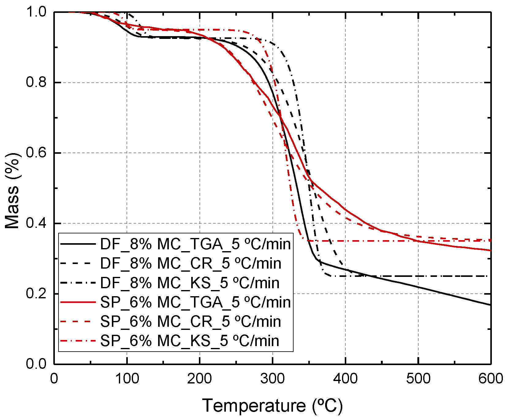
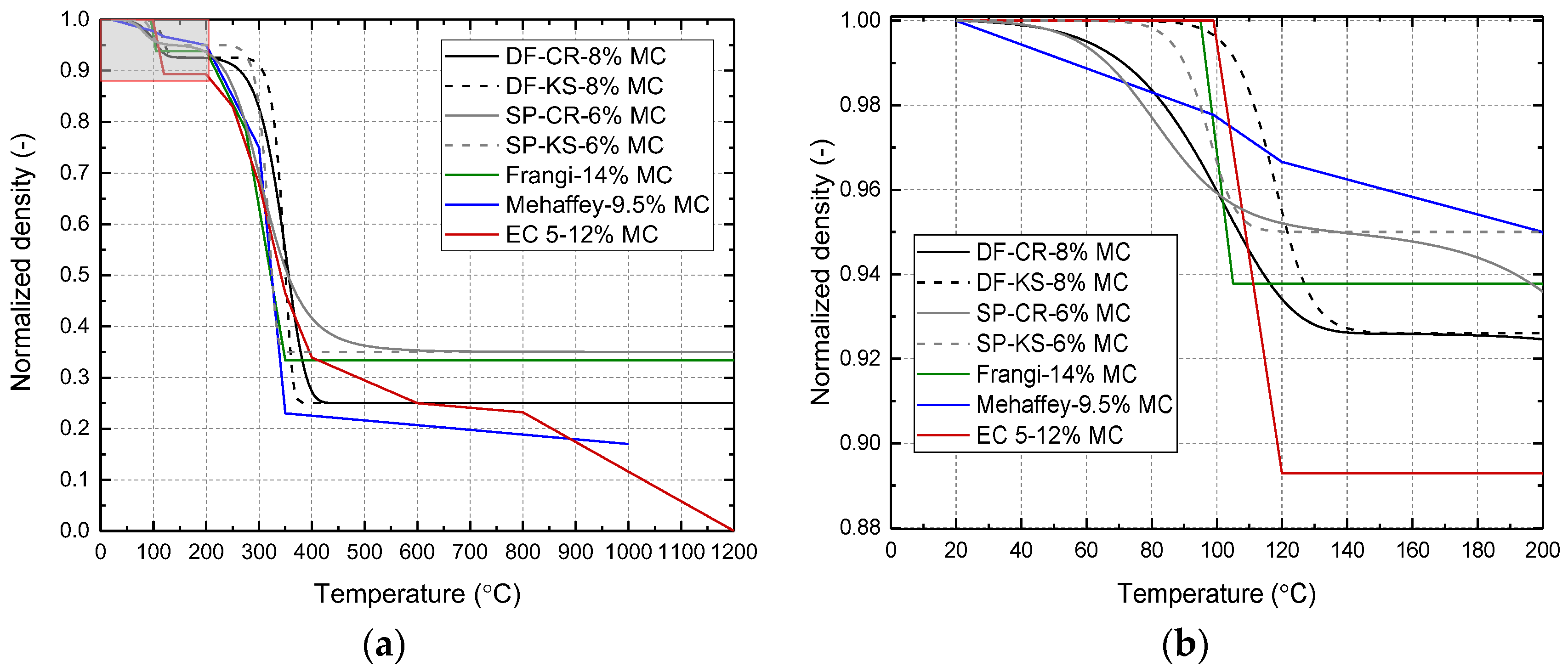
During the heating of wood, dehydration and pyrolysis are two key processes which have significant influence on the thermo-physical properties. The dehydration can be simply treated as a single-stage kinetic reaction of water, while the pyrolysis is much more complex since several pyrolysis reactions occur due to the simultaneous single-stage decompositions of hemicellulose, cellulose and lignin [18]. However, the mass loss of wood during pyrolysis generally exhibits a single stage for softwood [3], and hence the single-stage kinetic theory can be used to approximate the pyrolysis.

In this study, the wood is assumed to be composed of virgin wood, dehydrated wood and char. Hence, the conversion degrees of dehydration α_d and pyrolysis α_p can be expressed as

$$\begin{array}{l}{\alpha }_{\mathrm{d}}=\frac{{\rho }_{\mathrm{v}}-\rho }{{\rho }_{\mathrm{v}}-{\rho }_{\mathrm{d}}}\\ {\alpha }_{\mathrm{p}}=\frac{{\rho }_{\mathrm{d}}-\rho }{{\rho }_{\mathrm{d}}-{\rho }_{\mathrm{c}}}\end{array}$$

(1)

where ρ is the density; the subscripts v, d, c denote the virgin wood, dehydrated wood and char, respectively. The conversion degrees can be determined by the Arrhenius equations [16]:

$$\begin{array}{l}\frac{\partial {\alpha }_{\mathrm{d}}}{\partial t}=A_{\mathrm{d}}\exp \left(-\frac{E_{\mathrm{d}}}{RT}\right){\left(1-{\alpha }_{\mathrm{d}}\right)}^{n_{\mathrm{d}}}\\ \frac{\partial {\alpha }_{\mathrm{p}}}{\partial t}=A_{\mathrm{p}}\exp \left(-\frac{E_{\mathrm{p}}}{RT}\right){\left(1-{\alpha }_{\mathrm{p}}\right)}^{n_{\mathrm{p}}}\end{array}$$

(2)

where A, E and n are the frequency, activate energy and reaction order, respectively; R is the ideal gas constant; T is the temperature.

Douglas fir (DF) and Spruce (SP), i.e., the same types of wood used in the subsequent validation experiments, were selected to obtain the kinetic parameters. DF samples with an average density of 500 kg/m³ and a MC of 8% were used in TGA experiments at the heating rates of 5, 10 and 20 °C/min. The TGA curves of SP with a MC of 6%, subjected to the same heating rates, were adopted from literature [19]. The above mentioned heating rates were adopted since they generally covered the average heating rates of approximately 5 °C/min for the dehydration experiment and 15.4 °C/min for the standard fire experiment. The kinetic parameters of dehydration and pyrolysis of DF and SP were calculated based on these TGA measurements, using the modified Coats–Redfern (CR) [16,20] and Kissinger (KS) [21] methods; the results are shown in

Table 1. Kinetic parameters of dehydration and pyrolysis.

Specie	Model	Ad (Hz)	Ed (kJ/mol)	nd (-)	Ap (Hz)	Ep (kJ/mol)	np (-)
DF (8% MC)	CR	1.21 × 104	4.66 × 104	1.01	4.88 × 104	8.60 × 104	1.00
DF (8% MC)	KS	6.50 × 1022	1.83 × 105	1.70	8.20 × 1015	2.13 × 105	1.00
SP (6% MC)	CR	2.97 × 109	7.92 × 104	1.90	3.10 × 103	6.86 × 104	2.05
SP (6% MC)	KS	6.28 × 1025	1.96 × 105	1.52	2.08 × 1015	1.99 × 105	1.05

. During dehydration, the values of A and E obtained from the KS method were always higher than the counterparts from the CR method. The frequency factor, A, represents the intensity of the reaction while the activate energy, E, shows the energy required to activate the reaction. This indicates that the reactions described by the KS method were delayed and much more intensive compared to those from the CR method.

Substituting the kinetic parameters into Equation (2) allowed for calculating the conversion degrees. With the given conversion degrees of dehydration and pyrolysis, the temperature-dependent mass, M, could be expressed by [16]:

$$M=\left(1-{\alpha }_{\mathrm{d}}\right)M_{\mathrm{v}}+{\alpha }_{\mathrm{d}}\left(1-{\alpha }_{\mathrm{p}}\right)M_{\mathrm{d}}+{\alpha }_{\mathrm{d}}{\alpha }_{\mathrm{p}}{M}_{\mathrm{c}}$$

(3)

As shown in Figure 1, good agreements were found between the TGA and the modeling results calculated from the CR method, indicating that the model could capture the mass loss under dehydration and one-stage pyrolysis. The modeling curves obtained from the KS method, as derived before, exhibited a delay, but then a faster mass loss than measured, in both the dehydration and pyrolysis stages.

2.2. Density

During the dehydration and pyrolysis processes, the density can be expressed by:

$$\rho =\left(1-{\alpha }_{\mathrm{d}}\right){\rho }_{\mathrm{v}}+{\alpha }_{\mathrm{d}}\left(1-{\alpha }_{\mathrm{p}}\right){\rho }_{\mathrm{d}}+{\alpha }_{\mathrm{d}}{\alpha }_{\mathrm{p}}{\rho }_{\mathrm{c}}$$

(4)

where ρ is the apparent density; ρ_v is the density of virgin wood and depends on the MC; ρ_d is the density of dehydrated wood; ρ_c is the density of char, determined from the TGA results. The resulting normalized densities of the modeling results for DF (8% MC) and SP (6% MC) are shown in Figure 2, together with models from Frangi [9], Mehaffey [10] and Eurocode 5 (EC5) [11].

During the dehydration stage, the density of DF obtained from the KS method dropped from 80 to 125 °C while the density based on the CR method had a wider transition range from 30 to 125 °C. Similarly, the density of SP described by the KS method decreased from 70 to 110 °C while the density calculated by the CR method dropped from 40 to 160 °C. Although the modeling results based on the CR method had a better agreement with the TGA results than those based on KS, a better agreement was found between the KS results, EC5 and Frangi’s model, despite some differences in the MC, as seen in Figure 2b.

All models generally had a similar density evolution during pyrolysis. The density of DF obtained from the KS method dropped from 250 to 350 °C while that based on the CR method had a wider range from 200 to 400 °C. In the proposed model, based on the TGA results, the normalized density of char was assumed as 0.25 and 0.35 for DF and SP, respectively, and kept constant after pyrolysis. The density in Mehaffey’s proposal reduced linearly from 0.23 at 350 °C to 0.17 at 1000 °C while a constant value of 0.33 was adopted in Frangi’s model. The EC5 showed a multi-linear decrease in density, considering the formation of cracks in the char from 400 to 800 °C and the recession of the char from 800 to 1200 °C.

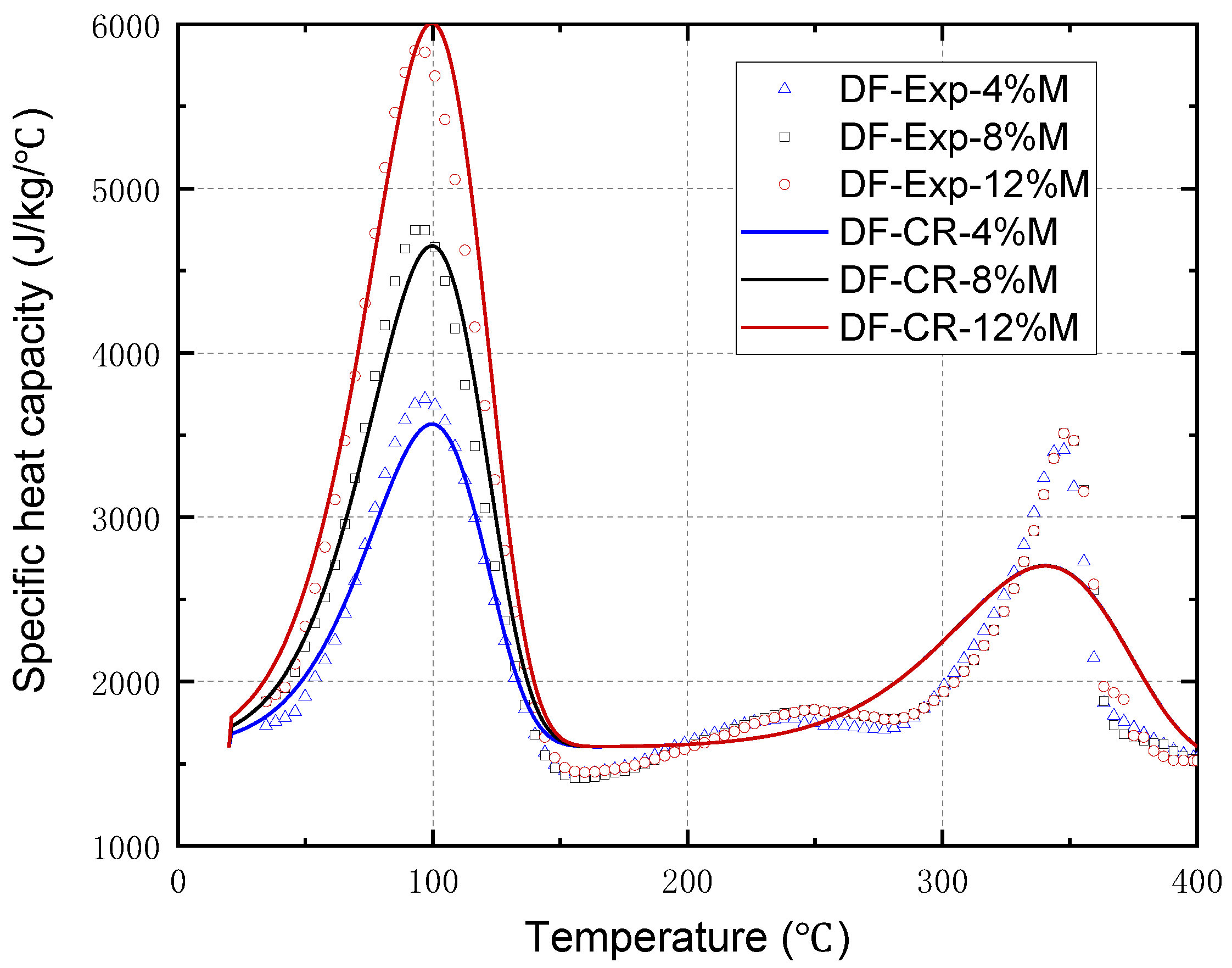
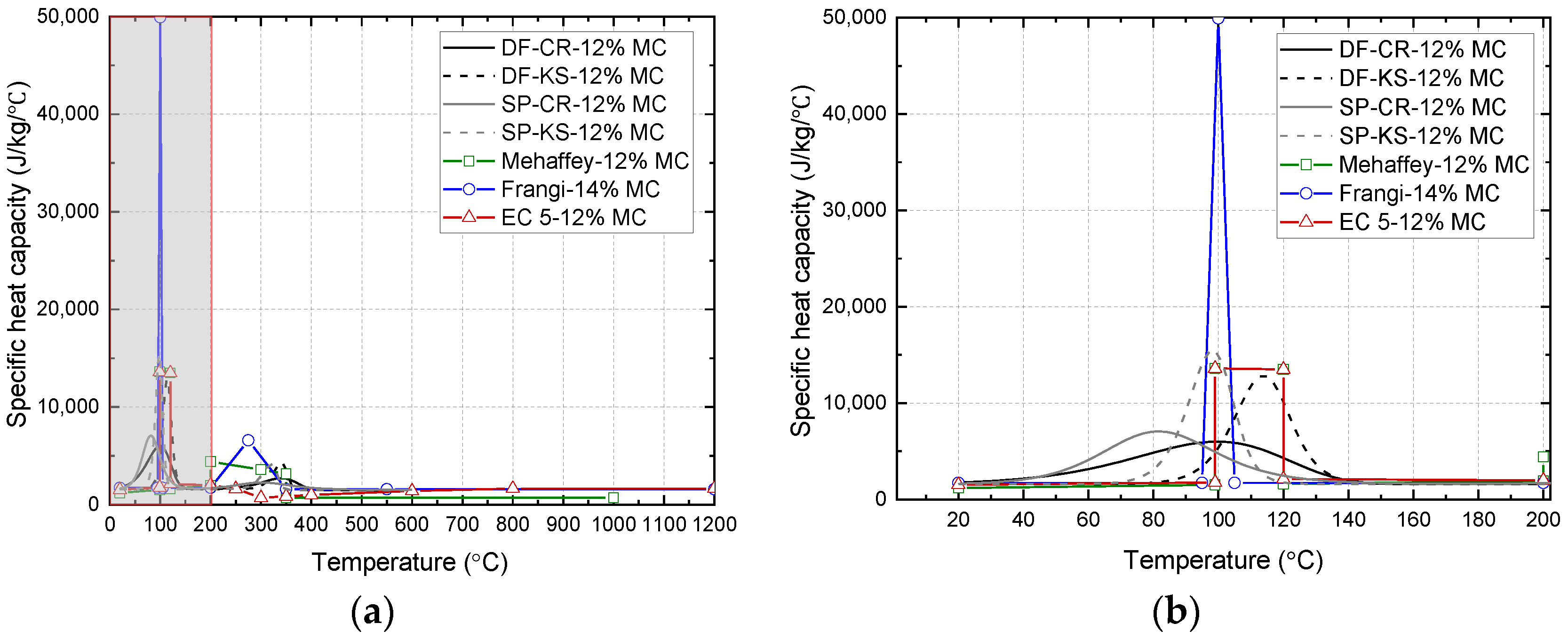
2.3. Specific Heat Capacity

The specific heat capacity can be defined as the amount of energy required to cause an increase of one unit of temperature in unit of mass. The apparent specific heat capacity of wood can be expressed as in Equation (5) considering the effect of latent heat (water evaporation heat) and pyrolysis heat [16]:

$$C_{\mathrm{p}}=\frac{\Delta Q}{\Delta TM}=\frac{\Delta Q_{\mathrm{m}}+\Delta Q_{\mathrm{d}}+\Delta Q_{\mathrm{p}}}{\Delta TM}$$

(5)

where ΔQ is the sum of the heat required to raise the temperature by ΔT of the material, ΔQ_m, the latent heat, ΔQ_d, and the pyrolysis heat, ΔQ_p. These terms can be expressed as:

$$\begin{array}{l}\Delta Q_{\mathrm{m}}=\left(C_{\mathrm{p},v}\left(1-{\alpha }_{\mathrm{d}}\right)M_{\mathrm{v}}+C_{\mathrm{p},\mathrm{d}}{\alpha }_{\mathrm{d}}\left(1-{\alpha }_{\mathrm{p}}\right)M_{\mathrm{d}}+C_{\mathrm{p},\mathrm{c}}{\alpha }_{\mathrm{d}}{\alpha }_{\mathrm{p}}{M}_{\mathrm{c}}\right)\Delta T\\ \Delta Q_{\mathrm{d}}={\alpha }_{\mathrm{d}}M{C}_{\mathrm{d}}\\ \Delta Q_{\mathrm{p}}={\alpha }_{\mathrm{p}}M{C}_{\mathrm{py}}\end{array}$$

(6)

where C_p,v, C_p,d and C_p,c are the specific heat capacities of the virgin wood, dehydrated wood and char, respectively. C_d and C_py denote the latent heat and pyrolysis heat of a unit mass. Substituting Equation (6) into Equation (5), the specific heat capacity can be expressed as:

$$C_{\mathrm{p}}=\frac{\Delta Q}{\Delta TM}=C_{\mathrm{p},\mathrm{v}}{f}_{\mathrm{v}}+C_{\mathrm{p},\mathrm{d}}{f}_{\mathrm{d}}++C_{\mathrm{p},\mathrm{c}}{f}_{\mathrm{c}}+\frac{\Delta {\alpha }_{\mathrm{d}}}{\Delta T}{C}_{\mathrm{d}}+\frac{\Delta {\alpha }_{\mathrm{p}}}{\Delta T}{C}_{\mathrm{py}}$$

(7)

where the mass fraction of virgin wood, dehydrated wood and char can be expressed as [16]:

$$\begin{array}{l}{f}_{\mathrm{v}}=\left(1-{\alpha }_{\mathrm{d}}\right)M_{\mathrm{v}}/\left[\left(1-{\alpha }_{\mathrm{d}}\right)M_{\mathrm{v}}+{\alpha }_{\mathrm{d}}\left(1-{\alpha }_{\mathrm{p}}\right)M_{\mathrm{d}}+{\alpha }_{\mathrm{d}}{\alpha }_{\mathrm{p}}{M}_{\mathrm{c}}\right]\\ f_{\mathrm{d}}={\alpha }_{\mathrm{d}}\left(1-{\alpha }_{\mathrm{p}}\right)M_{\mathrm{d}}/\left[\left(1-{\alpha }_{\mathrm{d}}\right)M_{\mathrm{v}}+{\alpha }_{\mathrm{d}}\left(1-{\alpha }_{\mathrm{p}}\right)M_{\mathrm{d}}+{\alpha }_{\mathrm{d}}{\alpha }_{\mathrm{p}}{M}_{\mathrm{c}}\right]\\ f_{\mathrm{c}}={\alpha }_{\mathrm{d}}{\alpha }_{\mathrm{p}}{M}_{\mathrm{c}}/\left[\left(1-{\alpha }_{\mathrm{d}}\right)M_{\mathrm{v}}+{\alpha }_{\mathrm{d}}\left(1-{\alpha }_{\mathrm{p}}\right)M_{\mathrm{d}}+{\alpha }_{\mathrm{d}}{\alpha }_{\mathrm{p}}{M}_{\mathrm{c}}\right]\\ f_{\mathrm{v}}=1-f_{\mathrm{d}}-f_{\mathrm{c}}\end{array}$$

(8)

Differential scanning calorimetry (DSC) experiments were conducted to obtain the true heat capacities (C_p,v, C_p,d and C_p,c), the latent heat C_d, and the pyrolysis heat C_py. DF samples with 4, 8 and 12% MC were scanned from 40 to 600 °C at a heating rate of 5 °C/min. It should be noted that the above mentioned MCs were determined according to the TGA curve. Nitrogen with a flow rate of 40 mL/min was used as the purge gas in order to simulate the inert environment of wood pyrolysis. Figure 3 shows the apparent specific heat capacity curves obtained from DSC.

The latent heat, C_d, can be obtained by integrating the DSC-measured heat from the onset to the end of dehydration and subtracting the true heat required for increasing the temperature of the material [16]. The corresponding values of the DF samples with 4, 8 and 12% MC were 95, 174 and 239 kJ/kg. The latent heat can also be calculated based on a given MC and the evaporation heat of water (2257 kJ/kg at 100 °C) [9]:

$$C_{\mathrm{d}}=2257\mathrm{kJ}/\mathrm{kg}\times \frac{w}{1+w}$$

(9)

where w denotes the MC. The corresponding calculated latent heat of wood with 4, 8 and 12% MC was 87, 167 and 242 kJ/kg, respectively. Good agreements were found between the latent heat based on DSC results and the values calculated from Equation (9).

The pyrolysis heat and the specific heat values of virgin wood, dehydrated wood and char were also determined based on the DSC curves. These values, the latent heat and the pyrolysis heat of DF are summarized in

Table 2. Values of specific heat capacity.

Specie	Cp,v J/(kg·K)	Cp,d J/(kg·K)	Cp,c J/(kg·K)	Cd kJ/kg	Cpy kJ/kg
DF	1600	1600	1500	Equation (9)	100
SP	1600	1600	1500	Equation (9)	100

. As shown in Figure 3, good agreements were found in the dehydration stage between the experimental and calculated results. In the pyrolysis stage, the model gave a reasonable agreement. The same parameters in Table 2 for calculating the apparent specific heat capacity were also adopted for SP, since the specific heat capacity of wood is practically independent of density or species [1]. Furthermore, in EC5 the specific heat capacity at room temperature was suggested to be 1530 kJ/(kg·K) [11] which is close to the value (1600 kJ/(kg·K)) adopted in this study.

The comparison between the proposed model of specific heat capacity for DF and SP, using the CR and KS methods, and models from literature [9,10,11] is shown in Figure 4. Instead of the 8% and 6% MCs used in TGA experiments for DF and SP, an identical 12% MC was selected by using the same MC in Equation (9). This value was selected since it was commonly adopted for calculating the apparent specific heat capacity [10,11]. In the dehydration stage, Frangi’s model showed a much higher peak value of 50 kJ/(kg·K) in a narrow temperature range from 94 to 104 °C, based on Equation (9), while the models of Mehaffey and EC5 exhibited the same peak value from 100 to 120 °C. For both DF and SP, the model using the KS method agreed well with EC5, while the model using the CR method had a lower peak value with a wider temperature range for dehydration. An additional pyrolysis heat of 370 kJ/ kg was suggested by Mehaffey, and was also used in Frangi’s model. However, König pointed out that this value is the energy absorbed per unit mass of volatile gas rather than per unit of wood [8,14]. Since it was disputed whether pyrolysis is endothermic or exothermic, the pyrolysis was usually neglected by the authors in [8,12,13,22]. This dispute may be related to the gas types using in the DSC since the pyrolysis usually shifted from one-stage endothermic reaction to two-stage exothermic reaction when changing the purge gas from inert gas such as nitrogen to oxidizing gas such as air or oxygen [23]. As shown in Figure 3, the DSC result of DF showed a clear endothermic reaction with a pyrolysis heat of approximately 100 kJ/ kg when using nitrogen.

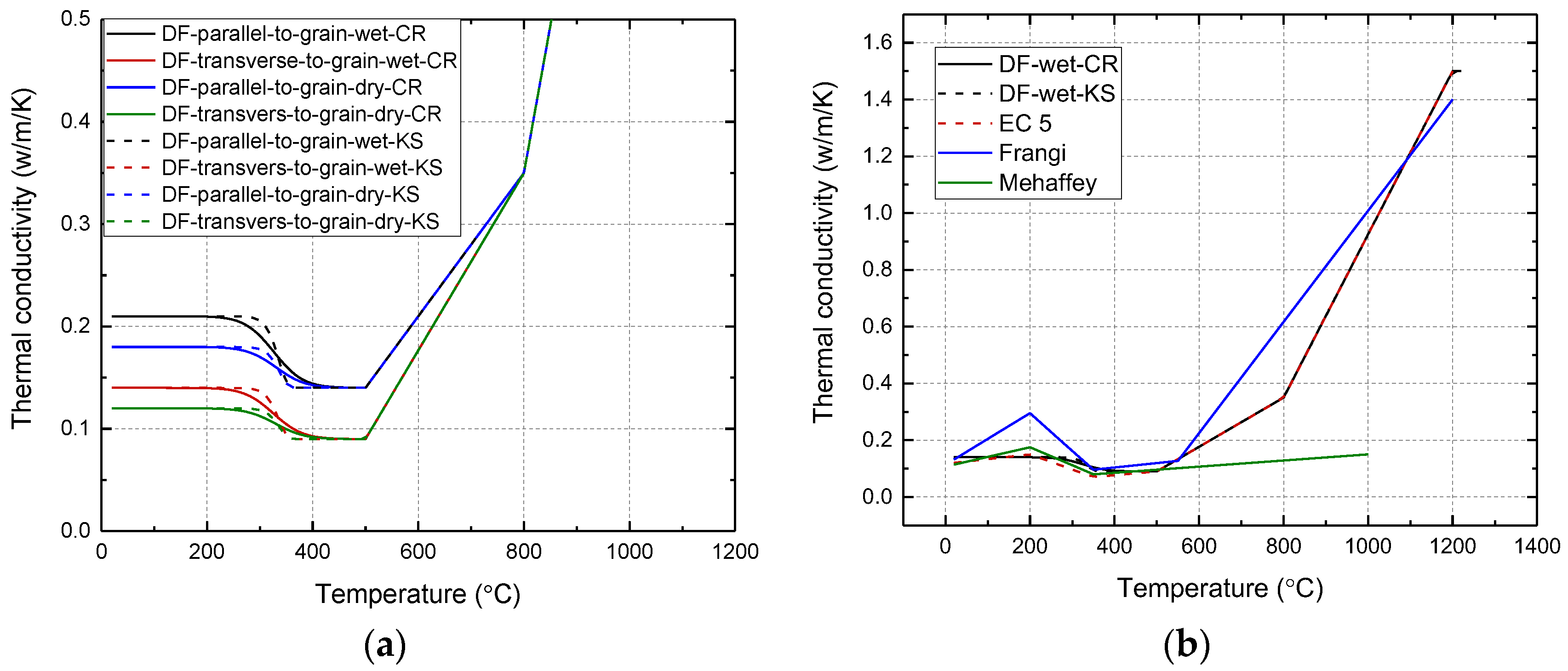
2.4. Thermal Conductivity

The thermal conductivity of wood in the parallel-to-grain direction is much higher than that in the radial and tangential directions due to its orthotropic nature [24]. Based on the inverse rule of mixture [16], the apparent thermal conductivity vector of wood can then be expressed as:

$$\begin{array}{l}{k}_{\mathrm{c}}=k_{L}i+k_{R}j+k_{T}k\\ =-\frac{1}{\frac{1-{\alpha }_{\mathrm{d}}}{k_{L,\mathrm{v}}}+\frac{{\alpha }_{\mathrm{d}}\left(1-{\alpha }_{\mathrm{p}}\right)}{k_{L,\mathrm{d}}}+\frac{{\alpha }_{\mathrm{d}}{\alpha }_{\mathrm{p}}}{k_{L,\mathrm{c}}}}i-\frac{1}{\frac{1-{\alpha }_{\mathrm{d}}}{k_{R,\mathrm{v}}}+\frac{{\alpha }_{\mathrm{d}}\left(1-{\alpha }_{\mathrm{p}}\right)}{k_{R,\mathrm{d}}}+\frac{{\alpha }_{\mathrm{d}}{\alpha }_{\mathrm{p}}}{k_{R,\mathrm{c}}}}j-\\ \frac{1}{\frac{1-{\alpha }_{\mathrm{d}}}{k_{T,\mathrm{v}}}+\frac{{\alpha }_{\mathrm{d}}\left(1-{\alpha }_{\mathrm{p}}\right)}{k_{T,\mathrm{d}}}+\frac{{\alpha }_{\mathrm{d}}{\alpha }_{\mathrm{p}}}{k_{T,\mathrm{c}}}}k\end{array}$$

(10)

where k_c is the thermal conductivity vector; i, j, k are the notations of standard base for the 3-D space; L, R, T denote the parallel-to-grain, radial and tangential directions.

A transversely isotropic thermal conductivity was adopted since there is no significant difference between the conductivity in radial and tangential directions [1]. Corresponding values at room temperature for wet (12% MC) and oven-dry (0% MC) DF and SP were adopted from the wood hand book [1] in

Table 3. Values of thermal conductivity.

Specie	w (%)	kL,v W/(m·K)	kL,d W/(m·K)	kL,c W/(m·K)	kT/R,v W/(m·K)	kT/R,d W/(m·K)	kT/R,c W/(m·K)
DF (12% MC)	12	0.21	0.21	0.14	0.14 [1]	0.14	0.09 [11]
DF (0% MC)	0	0.18	0.18	0.14	0.12 [1]	0.12	0.09 [11]
SP (12% MC)	12	0.18	0.18	0.14	0.12 [1]	0.12	0.09 [11]
SP (0% MC)	0	0.15	0.15	0.14	0.10 [1]	0.10	0.09 [11]

. The conductivity in the parallel-to-grain direction is higher than that in transverse direction [24,25,26,27]. According to the Forest Products Laboratory, the thermal conductivity along the grain is greater than conductivity across the grain by a factor of 1.5 to 2.8, with an average of about 1.8 [1]. However, a small range of ratios, as between 1.0 and 1.6, was reported by Yapici et al. [26]. In this study, the conductivity values of wood and char in parallel-to-grain direction were assumed 1.5 times that in the transverse direction. This value was also adopted by Fonseca and Barreira [27] to predict the char-layer evolution of pine wood by taking into account the grain orientations. The conductivity after dehydration was assumed to be equal to that of the virgin wood since the thermal conductivity increases only slightly from ambient temperature up to the end of dehydration in models such as Mehaffey and EC5. The value of char in the transverse directions was selected as 0.09 W/(m·K) according to EC5 and assumed to follow EC5 above temperatures of 500 °C where the char starts to crack.

The estimated thermal conductivity for wet and oven-dry DF is shown in Figure 5. Since the evolution of conductivity of SP is similar to that of DF, only the conductivity of DF is presented. The conductivity of parallel-to-grain was higher than that of transverse-to-grain. The conductivity of wet wood was furthermore higher than that of dry wood. However, the difference became smaller with the progress of pyrolysis. The values calculated with the CR method decreased slower than those obtained from the KS method. The comparison of the conductivity values of DF calculated by the proposed model and other models is shown in Figure 5b. The proposed model had smoother transitions but agreed well with EC5 and Mehaffey’s model up to 500 °C. The conductivity proposed by Frangi had higher values, especially around 200 °C, compared with the other models. Above 500 °C, the values rose fast due to the effects of crack and recession in the char which were not considered in Mehaffey’s model.

3. Numerical Modeling in Abaqus and OpenFOAM

In this study, the developed thermo-physical model was implemented in Abaqus and OpenFOAM to simulate the thermal responses of wood. Since OpenFOAM is based on the finite volume method, it is easier to simulate the gas flow in the wood compared to the Abaqus which is based on the finite element method. By comparing the numerical results from OpenFOAM and Abaqus, the accuracy of the numerical results can be guaranteed. Moreover, the developed thermophysical model can be verified by comparing the numerical results with the experiments.

3.1. Heat Transfer Model in Abaqus

A typical 3D heat transfer equation in differential form can be expressed as [28,29]:

$$C_{\mathrm{p}}\rho \frac{\partial T}{\partial t}=\frac{\partial }{\partial x}\left(k_{\mathrm{c},x}\frac{\partial T}{\partial x}\right)+\frac{\partial }{\partial y}\left(k_{\mathrm{c},y}\frac{\partial T}{\partial y}\right)+\frac{\partial }{\partial z}\left(k_{\mathrm{c},z}\frac{\partial T}{\partial z}\right)+Q_{\mathrm{r}}$$

(11)

where k_c,x, k_c,xy, k_c,z denote the thermal conductivities in three directions, i.e., x, y and z; Q_r is the total change of heat produced by physical or chemical processes per unit time. However, it is not easy to solve Equation (11) with temperature-dependent material properties and complex boundary conditions. In finite element software, such as Abaqus, the week form of Equation (11) is used [30]:

$$\frac{1}{\Delta t}{\displaystyle {\int }_V\delta T\rho }\left(U_{t+\Delta t}-U_t\right)\mathrm{d}V={\displaystyle {\int }_S\delta Tq}\mathrm{d}S+{\displaystyle {\int }_V\delta Tr}\mathrm{d}V+{\displaystyle {\int }_V\delta g\cdot F}\mathrm{d}V$$

(12)

where V and S denote the volume and the surface of the solid material; δT is an arbitrary variational temperature field satisfying the essential boundary conditions; U is the internal energy; t is time; Δt is the time step; q is the heat flux per unit area of the body, flowing into the body; r is the heat supplied internally into the body per unit volume; g denotes the temperature gradient; and F represents the heat flux vector.

The initial conditions can be described by:

$$T\left(x,y,z,t\right)\left|{ }_{t=0}\right.=T_0$$

(13)

where T₀ is the prescribed temperature at the start of the simulation. The boundary conditions can be prescribed temperature, T = T(x, y, z, t); or heat flux, q = q(x, y, z, t); or surface convection, q = h_conv (T − T_∞); or radiation, q = σ_sb ε_e (T⁴ − T_∞⁴). One of the frequently used boundary conditions is the combination of convection and radiation [31]:

$$q=h_{\mathrm{conv}}\left(T-T_{\infty }\right)+{\sigma }_{\mathrm{sb}}{\epsilon }_{\mathrm{e}}\left(T^4-T_{\infty }^4\right)$$

(14)

where h_conv is the convection coefficient; σ_sb is the Stefan–Boltzmann constant; ε_e is the emissivity; and T_∞ is the furnace temperature (hot face) or the ambient temperature (cold face).

3.2. Implementation in Abaqus

For the heat transfer analysis, the input parameters in Abaqus/CAE (Complete Abaqus Environment) are the density, specific heat capacity and thermal conductivity. However, the thermo-physical model composed of Equations (2), (4), (7) and (10) cannot be implemented directly in Abaqus since only piecewise functions of temperature are accepted. A previous developed user-defined subroutine of heat transfer (UMATHT) was thus presented [30], in which the conversion degrees of dehydration and pyrolysis were firstly calculated, followed by the calculation of the thermo-physical properties. To solve Equation (12), the following variables need to be defined in UMATHT [30]:

• Internal thermal energy, U;
• Variation of U with respect to temperature, ∂U/∂T;
• Variation of U with respect to the spatial gradients of temperature, ∂U/∂(∂T/∂x_i) (i = 1, 2, 3);
• Heat flux vector, F;
• Variation of F with respect to temperature, ∂F/∂T;
• Variation of F with respect to the spatial gradients of temperature, ∂F/∂(∂T/∂x_i) (i = 1, 2, 3).

These variables are functions of thermo-physical properties and must be defined at the end of each time step. The kinetic parameters obtained from the KS method for DF and SP were selected to calculate the corresponding dehydration degree α_d and pyrolysis degree α_p, according to Equation (2), since the peak of the specific heat capacity obtained with the KS method agreed well with other models (EC5 and Mehaffey). The apparent density, specific heat capacity and thermal conductivity were calculated according to Equations (4), (7) and (10), respectively. The effect of MC on the apparent density and specific heat capacity was considered by setting the virgin density ρ_v and dehydrated density ρ_d while the effect of MC on the apparent specific heat capacity was reflected in the dehydration heat C_d according to Equation (9). Finally, the variables related to U and F were thus obtained. In addition, the INP (input) file, providing the information about Geometry, material properties, mesh and boundary conditions, was generated by Abaqus/CAE. The Abaqus Standard solver was used to solve the discrete governing equations and finally the modeling results, including field variables (temperature) and user-defined variables, were obtained.

3.3. Heat Transfer Model in OpenFOAM

Abaqus Standard can provide solutions for most of the heat transfer problems in solids. However, it cannot independently solve the heat transfer in porous materials taking the effect of internal gas convection into account. In order to simulate the vapor and pyrolysis gas flow and quantify the effect of convection on the thermal responses in the porous wood, the open source finite volume software OpenFOAM [32], which has the capacity to solve fluid dynamic problems, was used. In OpenFOAM, a set of governing equations, including the mass conservation, gas (vapor) momentum conservation, and the energy conservation can be easily integrated. In this study, the concept of virtual gas mixture phase, consisting of water vapor and pyrolysis gases, was used, i.e., the flowing medium was a gas mixture rather than individual vapor and pyrolysis gases. In the simulation, the physical properties of air were used for the gas mixture. The gaseous mass conservation equation is [33]:

$$\frac{\partial ({ϵ}_{\mathrm{g}}{\rho }_{\mathrm{g}})}{\partial t}+\frac{\partial ({ϵ}_{\mathrm{g}}{\rho }_{\mathrm{g}}{v}_{\mathrm{g},x})}{\partial x}+\frac{\partial ({ϵ}_{\mathrm{g}}{\rho }_{\mathrm{g}}{v}_{\mathrm{g},y})}{\partial y}+\frac{\partial ({ϵ}_{\mathrm{g}}{\rho }_{\mathrm{g}}{v}_{\mathrm{g},z})}{\partial z}=-\frac{\partial {\rho }_{\mathrm{s}}}{\partial t}$$

(15)

where ε_g, ρ_g, v_g are the porosity, density, and velocity of gas, respectively; ρ_s is the density of wood; t is the time; x y z denote the directions. The source term (right hand side) represents the production rate of the gas mixture and can be expressed as:

$$\frac{\partial {\rho }_{\mathrm{s}}}{\partial t}=\left({\rho }_{\mathrm{d}}-{\rho }_{\mathrm{v}}\right)\frac{\partial {\alpha }_{\mathrm{d}}}{\partial t}+\left({\rho }_{\mathrm{c}}-{\rho }_{\mathrm{d}}\right)\frac{\partial {\alpha }_{\mathrm{p}}}{\partial t}$$

(16)

where ρ_v is the density of virgin wood; ρ_d is the density of dehydrated wood; ρ_d is the density of char; α_d and α_p are the dehydration degree and pyrolysis degree, respectively.

The average gas velocity is obtained by resolution of the momentum-conservation equation based on Darcy’s law. In porous media, the volume-averaged momentum conservation can be written as [34,35]:

$$v_{\mathrm{g},x}=-\frac{K}{{ϵ}_{\mathrm{g}}\mu }\frac{\partial P}{{\partial }_{\mathrm{x}}}$$

(17)

where P is the gas pressure; μ is the viscosity coefficient; K is the permeability, a second order tensor, which can be calculated by the rule of mixture:

$$K=\left(1-{\alpha }_{\mathrm{d}}\right)K_{\mathrm{v}}+{\alpha }_{\mathrm{d}}\left(1-{\alpha }_{\mathrm{p}}\right)K_{\mathrm{d}}+{\alpha }_{\mathrm{d}}{\alpha }_{\mathrm{p}}{K}_{\mathrm{c}}$$

(18)

where K_v, K_d, K_c denote the permeability values of virgin wood, dehydrated wood and char. The Darcian velocity can be introduced in the gas mass conservation under the assumption that the perfect gas law holds [36]:

$$\frac{\partial }{\partial t}\left(\frac{{ϵ}_{\mathrm{g}}M}{RT}P\right)-\frac{\partial }{\partial x}\left(\frac{PM}{RT}\left(\frac{1}{\mu }K+\frac{1}{P}\beta \right){\partial }_{\mathrm{x}}P\right)=\left({\rho }_{\mathrm{v}}-{\rho }_{\mathrm{d}}\right)\frac{\partial {\alpha }_{\mathrm{d}}}{\partial t}+\left({\rho }_{\mathrm{d}}-{\rho }_{\mathrm{p}}\right)\frac{\partial {\alpha }_{\mathrm{p}}}{\partial t}$$

(19)

where M is the mean molar mass of the gas mixture; R is the ideal gas constant.

Under the local thermal equilibrium assumption, the energy conservation can be written as:

$$C_p\rho \frac{\partial T}{\partial t}+\left(\frac{\partial {ϵ}_{\mathrm{g}}{\rho }_{\mathrm{g}}{h}_{\mathrm{g}}{v}_{\mathrm{g},x}}{\partial x}+\frac{\partial {ϵ}_{\mathrm{g}}{\rho }_{\mathrm{g}}{h}_{\mathrm{g}}{v}_{\mathrm{g},y}}{\partial y}+\frac{\partial {ϵ}_{\mathrm{g}}{\rho }_{\mathrm{g}}{h}_{\mathrm{g}}{v}_{\mathrm{g},z}}{\partial z}\right)=\frac{\partial }{\partial x}\left(k_x\frac{\partial T}{\partial x}\right)+\frac{\partial }{\partial y}\left(k_y\frac{\partial T}{\partial y}\right)+\frac{\partial }{\partial z}\left(k_z\frac{\partial T}{\partial z}\right)$$

(20)

where h_g is the specific enthalpy of gas.

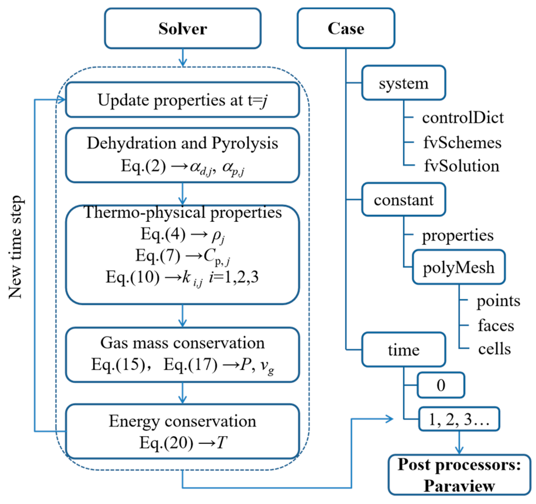
3.4. Implementation in OpenFOAM

OpenFOAM platform was adopted to solve the governing Equations (19) and (20). Figure 6 presents the general structure of a typical OpenFOAM analysis, which consists of “system”, “constant” and “time”. The function of the “system” including “controlDict”, “fvSchemes” and “fvSolution” is to set the time steps, discretization schemes, and linear solvers. The “constant” consists of “properties” providing the input parameters regarding the material properties of wood and gas and “polyMesh” providing the grid mesh. The “time” consists of the initial condition “0” and the results at each time step. Figure 6 also illustrates the numerical algorithm of the solver. The kinetic equations of dehydration and pyrolysis, the gas mass conservation equation and the energy conservation equation are solved in sequence according to the set of “system”. The numerical results are passed into the specific folders at each time step. Paraview software 5.5.2 [37] is used as the post-processor to display the simulation results.

4. Dehydration Experiments and Validation of Numerical Models

4.1. Dehydration Experiments under Elevated Temperature

4.1.1. Materials and Specimens

Cubic Douglas fir blocks with a side length of 88 mm were used as specimens. Holes were drilled for the installation of thermocouples and subsequently the blocks were stored in a conditioning room with a relative humidity of 65% and temperature of 20 °C for 4 weeks. After conditioning, the average density was 581 kg/m³ with a standard deviation (SDV) of 57.5 kg/m³ and the average MC was 13.7% with a SDV of 0.3%, according to the ASTM D4442 [38]. The specimen details are summarized in

Table 4. Experimental details of the dehydration and fire (pyrolysis) experiments.

Specimen	Exposed Surfaces	Dimension mm	Specie
DF block (13.7%MC)	6	88 × 88 × 88	Douglas fir
DF block (0% MC)	6	88 × 88 × 88	Douglas fir
CLT panel (12% MC)	1	2500 × 600 × 150	Spruce

. A total of four specimens including two wet specimens (13.7% MC) and two dry specimens (0% MC) were tested.

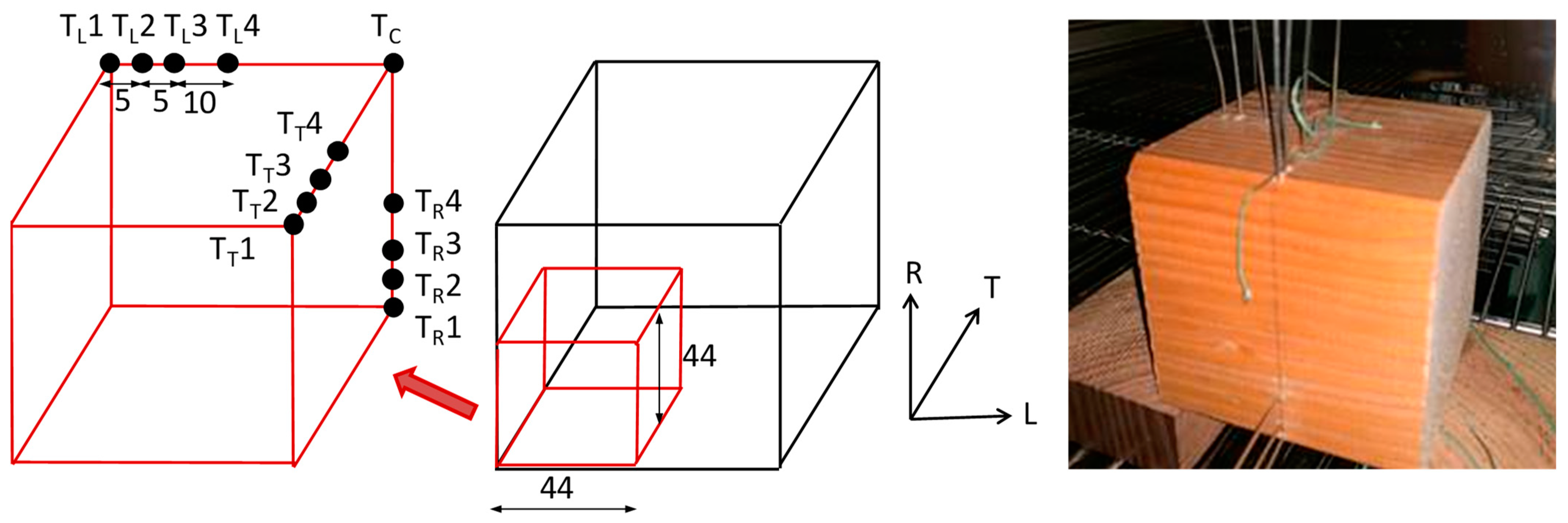
4.1.2. Set-Up and Experimental Program

As shown in Figure 7, a total of ten type K thermocouples with a probe diameter of 1.5 mm, supplied by Metra instruments, were placed along the three main orthogonal axes: longitudinal (L), Radial (R) and tangential (T). For each axis (L, R and T), four thermocouples were installed at the depths of 0, 5, 10 and 20 mm from the surface. The thermocouples were labeled as T_L1-4, T_R1-4 and T_T1-4, respectively, with the subscripts representing the direction of axis, while one thermocouple, labeled as T_c, was placed in the center.

The timber blocks with thermocouples were placed in the center of the oven and supported by two pieces of timber to avoid the contact with the steel frame. For the two wet specimens, the temperature then increased from room temperature (25 ± 2 °C) to 200 °C at a heating rate 3.9 °C/min. For the dry specimens, the specimens were first heated up to 150 °C for 5 h and then sealed with plastic bags to prevent the samples from the absorption of moisture. The totally dried samples were then heated again to 200 °C at a heating rate of 4.9 °C/min. The target temperature was 200 °C; however, the measured averaged oven temperatures for the wet and dry specimens were 180 and 195 °C. The heating program is summarized in

Table 5. Heating program of the DF specimens.

ID	Moisture Content (%)	Heating Time (min)	Target Temperature (°C)
S1-13.7%	13.7	120	200
S2-13.7%	13.7	120	200
S3-0%	0	120	200
S4-0%	0	120	200

.

4.1.3. Description of Numerical Modeling

The numerical study was carried out in both Abaqus and OpenFOAM. The kinetic parameters of DF calculated by the KS method were used, as mentioned above and listed in Table 1. The thermo-physical properties of DF with 13.7 and 0% MC were calculated for wet and dry DF specimens, respectively, according to Equations (4), (5) and (10) and then implemented in Abaqus and OpenFOAM.

One eighth of the block was modeled due to the symmetry of the specimen and boundary conditions, as shown in Figure 7. Eight-node linear brick elements “DC3D8” and eight-node “hex block” elements were used in Abaqus and OpenFOAM, respectively. A total of 10648 elements with a size of 2 mm were used in both models. The initial temperature was set as 25 °C. Based on the average measured air temperatures, the linear heating curves with the heating rates 3.9 and 4.9 °C/min were set as the boundary of the hot faces of the wet and dry specimens, respectively. The inner faces were set as the symmetry boundaries. In OpenFOAM, the initial and boundary conditions of gas pressure were also required. The air pressure, 101 kPa [36], was used for the initial gas pressure inside the wood and the boundary gas pressure of the hot faces. The required input parameters are summarized on

Table 6. Input parameters for numerical simulations.

Symbol	Parameter	Value			Units	Refs.
		Wet DF	Dry DF	SP
ρv	Density of virgin wood	581	510	449	kg/m3	[17]
ρd	Density of dehydrated wood	510	510	401	kg/m3
ρc	Density of char	116	116	90	kg/m3
w	Moisture content	13.7	0	12	%	[17]
Cp,v	Specific heat of virgin wood	1600	1600	1600	kJ/(kg·K)
Cp,d	Specific heat of dehydrated wood	1600	1600	1600	kJ/(kg·K)
Cp,c	Specific heat of char	1500	1500	1500	kJ/(kg·K)
Cd	Latent heat	272	0	242	kJ/kg
Cpy	Pyrolysis heat	100	100	100	kJ/kg
kL,v	Longitudinal wood conductivity	0.21	0.18	0.15	W/(m·K)
kR/T,v	Transverse wood conductivity	0.14	0.12	0.10	W/(m·K)	[1]
kL,c	Longitudinal char conductivity	0.14	0.14	0.14	W/(m·K)
kR/T,c	Transverse char conductivity	0.09	0.09	0.09	W/(m·K)	[11]
KL,v	Longitudinal wood permeability	7.5 × 10−13	7.5 × 10−13	7.5 × 10−13	m2	[39]
KR/T,v	Transverse wood permeability	7.5 × 10−13	7.5 × 10−13	7.5 × 10−13	m2	[39]
KL,c	Longitudinal char permeability	1.0 × 10−11	1.0 × 10−11	1.0 × 10−11	m2	[40]
KR/T,c	Transverse char permeability	1.0 × 10−11	1.0 × 10−11	1.0 × 10−11	m2	[40]
εg,v	Porosity of virgin wood	0.51	0.51	0.51		[39]
εg,c	Porosity of char	0.85	0.85	0.85		[39]
μ	Viscosity coefficient of gas	1.85 × 10−5	1.85 × 10−5	1.85 × 10−5	kg/(m s)
M	Mean molar mass of gas	0.028	0.028	0.028	kg/mol
R	Ideal gas constant	8.314	8.314	8.314	J/(mol·K)
σsb	Stefan–Boltzmann constant	5.67 × 10−8	5.67 × 10−8	5.67 × 10−8	W/(m2·K4)

. The simulations were conducted for 2 h with a time step of 0.5 s to avoid convergence problems.

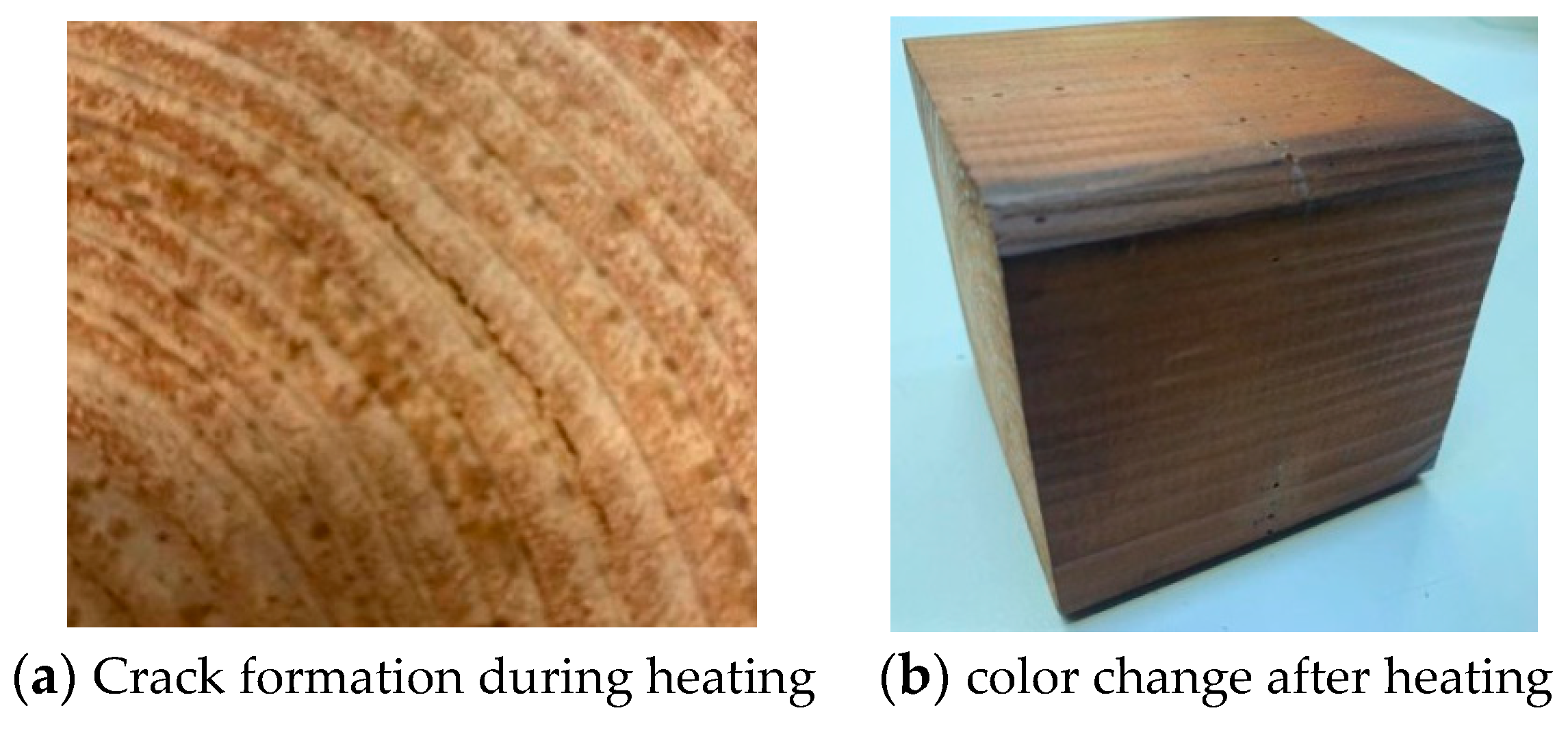
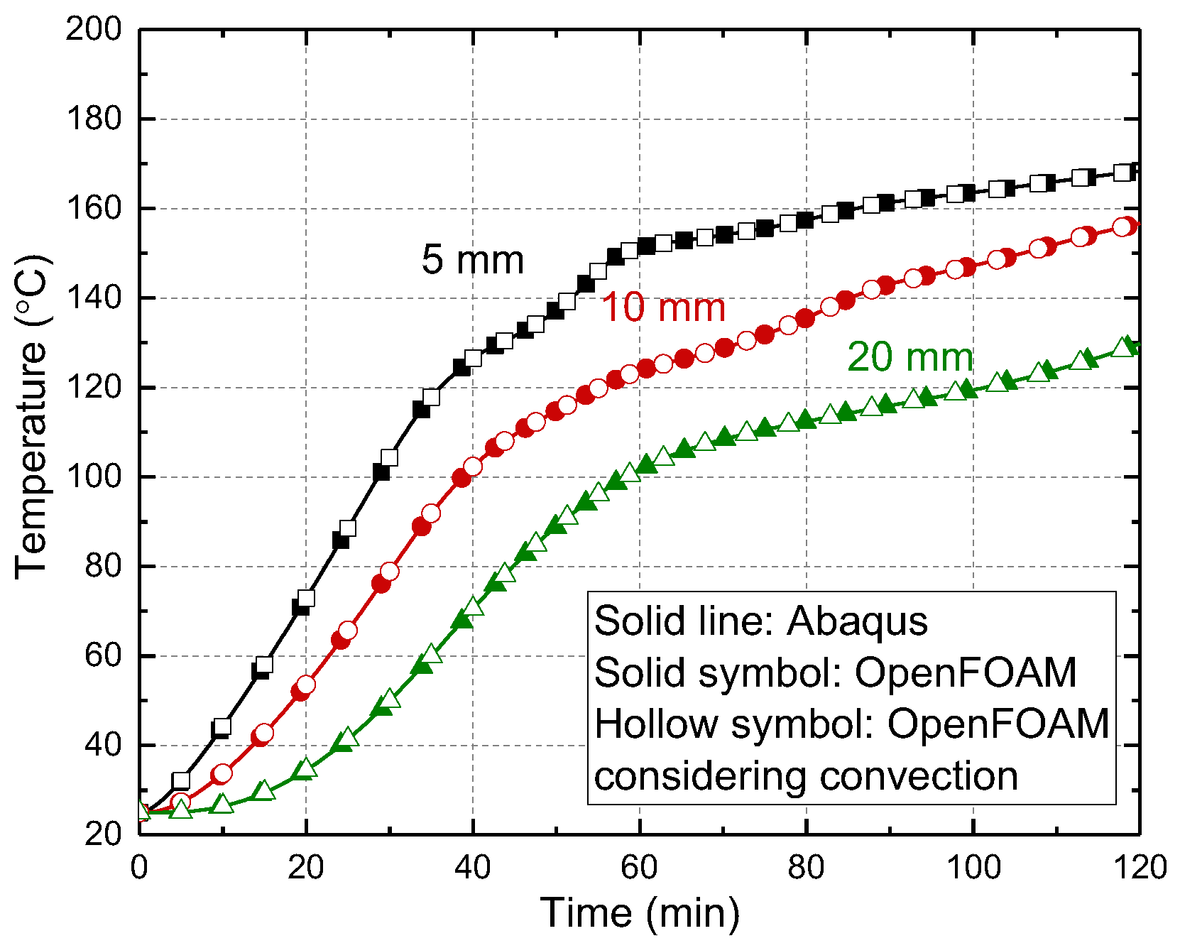
4.1.4. Comparison between Experimental and Numerical Results

Figure 8a presents the experimental temperature progressions of T_T (in transverse direction) and T_L (in longitudinal direction) of specimen S1 since specimens S1 and S2 gave similar results. The measured oven temperature (0 mm depth) increased almost linearly up to 180 °C in approximately 40 min. The internal temperatures also exhibit linear increments below approximately 100 °C, exhibiting an initial thermal lag. However, the internal temperatures increase slowly at around 100 °C due to the effect of dehydration. During this stage, several small tangential cracks were formed, as shown in Figure 9a. Subsequently, the rate of temperature increase slowed down, and, as a result of the dehydration, the center temperature T_c reached only about 110 °C after heating for 120 min. Regarding the effect of grain direction on the temperature progressions, the results were not consistent, i.e., the values of T_L were not always higher than those of T_T at the same depth from the hot face. This may have resulted from the small scale of the specimen or the uneven gas temperatures on the hot faces (Figure 8).

Figure 8b shows the experimental temperature progressions of T_T and T_L of specimen S3 (specimen S4 was not shown since the results are similar with specimen S3). The measured oven temperatures increased linearly up to 195 °C. The internal temperatures increased continuously during the whole heating time. At 120 min, the center temperature T_c reached approximately 190 °C. No significant differences between T_L and T_T measurements were found, indicating that the grain direction had little effect on the temperature progressions. This may be attributed to the small scale of the specimen or the uneven gas temperatures on the hot faces.

Comparing wet and dry specimens, the experimental temperature progressions in the former were delayed compared to the latter. After the heating of 120 min, the temperature in the dry specimen was higher than 180 °C everywhere while the temperature in the center part of wet specimens was only around 110 °C. A similar color change was observed in all specimens, as shown in Figure 9b.

Figure 8 also shows the comparison of the numerical results from Abaqus and the experimental results. Reasonable agreements were found between the modeling and the experimental temperatures. The latter were slightly overestimated up to 20 mm depth due to the above-mentioned thermal lag, which shifted the curves to slightly lower temperatures. The center temperature T_C was underestimated during 30–70 min. However, the discrepancy became smaller with the time. In addition, the modeling values of T_L were, consistently, slightly higher than those of T_R or T_T. Despite of the shift caused by the thermal lag and an obvious overestimation for T_C, the numerical results agreed well with the experimental temperatures, indicating that the proposed thermo-physical model can generally well predict the temperature progressions in both wet and dry DF specimens during the dehydration stage.

Figure 10 compares the numerical results obtained from Abaqus and OpenFOAM, without and with considering gas convection, for specimen S1 in transverse direction. Both simulations gave the same results without considering gas convection. Furthermore, the numerical results with and without considering gas convection almost overlapped, indicating that the gas convection had little effect on the temperature progressions.

The dehydration degree contours simulated by OpenFOAM at 0, 30, 60 and 120 min are shown in Figure 11. At the beginning, no dehydration occurred. At 30 min, obvious dehydration was found on the hot face. As the heat flux continuously penetrated into the wood, the dehydration front zone moved from the hot face towards the deeper area. At 120 min, the wood was almost fully dehydrated.

The gas pressure and velocity contours of specimen S1 at 0, 30, 60 and 120 min are presented in Figure 12. The pressure is represented by the color of the block while the gas velocity is indicated by the color of the arrows. At the start of the experiment, the initial pressure is 101 kPa and the gas (vapor) velocity is 0 m/s. With the progressions of dehydration, the gas is released, resulting in gas pressure along the paths from dehydration front zone to hot surfaces. At 30 min, the area close to hot surfaces undergoes intensive dehydration, and therefore, the gas moves along the pressure gradient and finally exhausts out normally to the hot surfaces. The dehydration front zone migrates toward the center of the specimen with the heat transfer process. At 60 min, the maximum pressure is located at the center of the specimen. As a result, the gas continuously flows out from the center towards the hot face. At 120 min, the magnitudes of the gas pressure and velocity are very low since the dehydration is nearly finished.

4.2. Fire Experiments on Full-Scale CLT Panel

4.2.1. Description of Experimental Program

A fire experiment on a full-scale cross-laminated timber (CLT) panel made of spruce was conducted by Frangiacomo et al. [17]. The 150 mm-thick panel consisted of 5 layers with different thicknesses at 42, 19, 28, 19 and 42 mm in the transverse direction. The dimensions of the panel are given in Table 4. The thermocouples were placed at the depths of 21, 52, and 75 mm from the hot face with 3 thermocouples placed in each depth. The bottom face of the panel was exposed directly to the ISO834 standard fire [41].

4.2.2. Description of Numerical Modeling

Specimen symmetry allowed for modeling only half of the transverse cross-section. A total of 45,000 4-node linear brick elements “DC2D8” with an element size of 1 mm along the depth and width, respectively, were used in Abaqus, while a total 45,000 8-node “hex block” elements with the same size were used in OpenFOAM. In both Abaqus and OpenFOAM, the initial temperature was set as ambient temperature of 0 °C according to the experiment [17]. Convection and radiation boundary conditions were used on the bottom and top surfaces. The convection coefficients were set as 25 and 4 W/(m² K), respectively, and the corresponding radiation coefficient was selected as 0.8, according to EC5. The side faces were set as adiabatic boundaries. Regarding the modeling in OpenFOAM, the initial gas pressure was set as 101 kPa on the bottom and top faces. As shown in Figure 13, the oven temperature generally followed the ISO834 curve except for the first 5 min, during which the oven temperature was much lower than the ISO curve and increased almost linearly up to approximately 580 °C. In order to obtain the precise boundary conditions, the input fire curve consisted of a linear part from ambient temperature to 580 °C, followed by the ISO curve. The thermo-physical properties of SP were calculated as completed for DF; the values used for the simulation are shown in Table 6. The simulations were run for 1h with a time step of 1 s.

4.2.3. Comparison between the Experimental and Numerical Results

The experimental curves at the depth of 21 mm exhibited a plateau at around 100 °C, followed by a quick increase in temperature. At 60 min, the temperatures at the depth of 52 mm were still below 100 °C. Good agreements were found between the modeling and experimental results, except an underestimation at the 21 mm depth from 0 min to 25 min. This discrepancy came from the difference of the temperature intervals of dehydration between the model and experiment. The experimental temperature curve at the 21 mm exhibited dehydration started at approximately 100 °C. However, in the simulation, based on the TGA experiments, as indicated in Figure 2b, an interval between 70 and 110 °C was used for calculating the thermo-physical properties, resulting in a smaller increment of temperature compared with the experimental values below 100 °C. The sample geometry adopted in the TGA test may have an effect on the temperature intervals of dehydration. The solid and big-size sample may lead to a delayed dehydration (the temperature plateau occurs around 100 °C) while the powdered and smaller sample may lead to an earlier dehydration.

Figure 13b shows the comparison of the numerical results from Abaqus and OpenFOAM without and with considering gas convection. The temperature curves obtained from Abaqus, OpenFOAM, without and with considering convection, almost overlapped, indicating that both software packages gave almost the same modeling results while gas convection had little effect on the temperature progressions.

The dehydration and pyrolysis degrees at 0, 30 and 60 min are shown in Figure 14. During the heating of the panel, the dehydration and the pyrolysis fronts were clearly identified. Furthermore, the dehydrated zone was much larger than the decomposed (char) zone at the same moment.

The gas pressure and velocity contours at 0, 30 and 60 min are presented in Figure 15. The magnitudes of the gas pressure and velocity are represented by the colors of the panel and the arrows, respectively. At the beginning of the modeling, the initial gas velocity is 0 m/s since no phase change occurred. During the heating process, the gas released by the dehydration and pyrolysis flowed along the pressure gradient since both the hot face and cold face had lower pressure. One part of the gas flowed toward the hot face while the other part flowed along the opposite way to the cold face. The reason for the little effect of convection came from the slow gas velocity (the maximum value was less than 14 mm/s at 60 min), as shown in Figure 15, since the velocity plays an important role in the convection term in Equation (20).

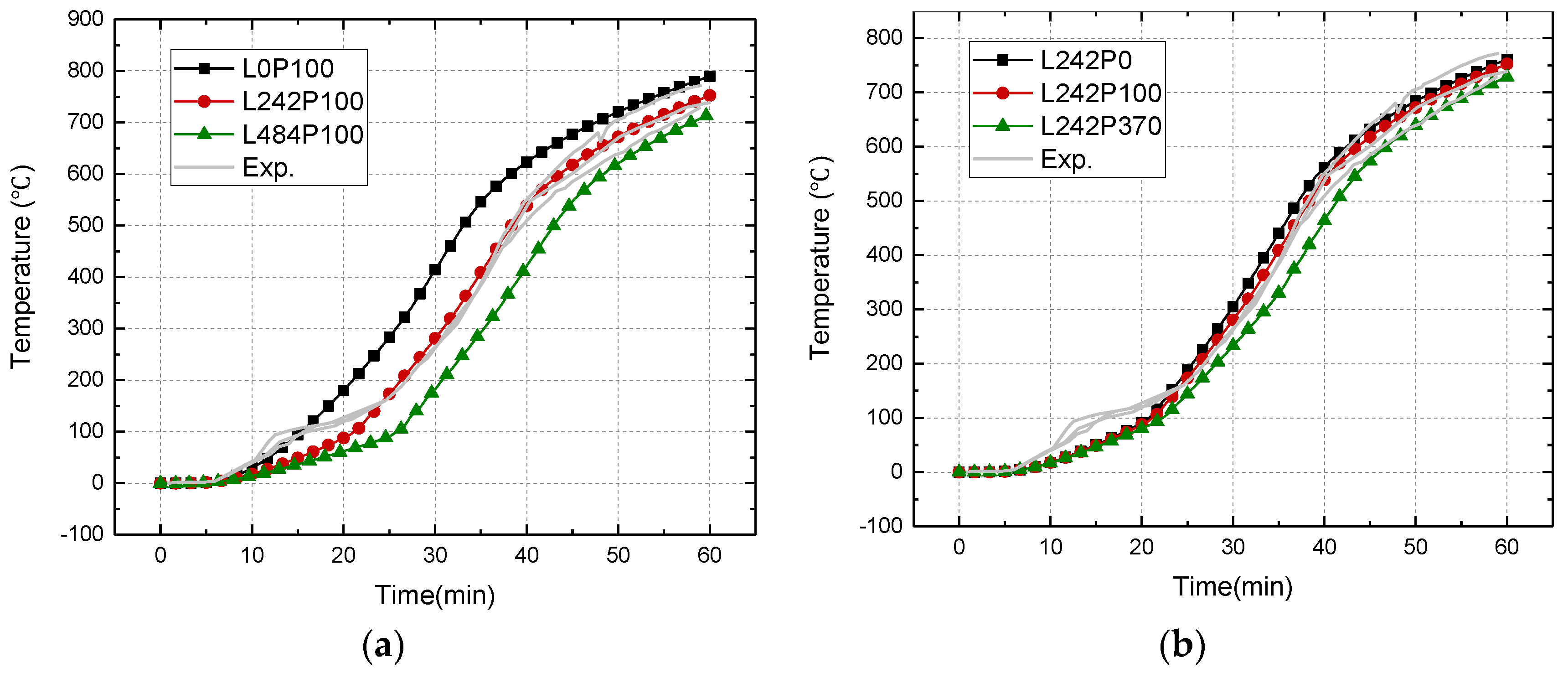
4.2.4. Effect of Latent Heat and Pyrolysis Heat

The fire experiment on the CLT panel was also used to conduct a parametric analysis, in order to investigate the effect of the latent heat and pyrolysis heat on the temperature progressions. The parametric analysis was divided into two groups. In the first group, 0, 242 and 484 kJ/kg were used as the latent heat, corresponding to MCs of 0, 12 and 24% (acc. to Equation (9)), while a constant value of 100 kJ/kg was set as the pyrolysis heat. In the second group, a constant value of 242 kJ/kg was used for the latent heat combined with the three values 0, 100, 370 kJ/kg for the pyrolysis heat. The combinations of the latent and pyrolysis heats are listed in

Table 7. Combinations of latent heat and pyrolysis heat for parametric study.

Group	Combination	MC (%)	Latent Heat (kJ/kg)	Pyrolysis Heat (kJ/kg)
1	L0P100	0	0	100
	L242P100	12	242	100
	L484P100	24	484	100
2	L242P0	12	242	0
	L242P100	12	242	100
	L242P370	12	242	370

.

Figure 16a depicts the comparison of the temperature profiles at the 21 mm depth between the experimental and numerical results using the three combinations of Group 1. With the increase in latent heat, an obvious delay in time (to reach the same temperature) occurred. For example, the time required to raise the temperature to 100 °C for L0P100, L242P100 and L484P100 were 16, 22 and 27 min, respectively. This delay was maintained until the end of the modeling. Figure 16b shows the effect of the pyrolysis heat on the temperature profiles. A delay in time with the increasing pyrolysis heat was shown from approximately 20 to 60 min. However, this delay was much shorter than that caused by the increase in dehydration heat.

5. Conclusions

Based on the experimental and numerical studies, the following conclusions are drawn.

• The thermo-physical model of wood considering moisture content was developed based on the kinetic theory. Unlike the frequently used thermo-physical properties based on the piecewise linear functions of temperature, the proposed thermo-physical properties are continuous and exhibit obvious physical meaning.
• The apparent specific heat capacity model of wood with different moisture contents was validated by the differential scanning calorimetry experiments on the Douglas fir wood. The apparent specific heat capacity of the Douglas fir wood obviously increased from approximately 3700 kJ/(kg·K) to 6000 kJ/(kg·K) as the moisture content increased from 4% to 12%. Moreover, the apparent specific heat capacity also significantly increased during the pyrolysis process.
• Apparent specific heat capacity was recommended in the simulation of thermal responses of wood since both latent heat and pyrolysis heat have significant effects on the thermal responses of wood. The wood with high moisture content absorbed more latent heat through dehydration compared to that with low moisture content, exhibiting a relatively low increasement in temperature near 100 °C during the heating process. The temperature progression is more sensitive to the latent heat than to the pyrolysis heat.
• The thermo-physical model was successfully implemented in open-source finite volume software, OpenFOAM, which can simulate three-dimensional gas flow inside porous wood. The effect of convection of gas on the temperature progressions depends on the gas velocity and enthalpy. The low gas pressure led to a low gas velocity in the dehydration and pyrolysis stages. Therefore, the gas convection seems to have limited influence on the temperature progressions.

References

1. Ross, R.J. Wood Handbook: Wood as an Engineering Material; U.S. Department of Agriculture, Forest Service, Forest Products Laboratory: Madison, WI, USA, 2010.
2. Zhang, F.; Lu, Z.; Wang, D.; Fang, H. Mechanical properties of the composite sandwich structures with cold formed pro-filed steel plate and balsa wood core. Eng. Struct. 2024, 300, 117256. [Google Scholar] [CrossRef]
3. Grønli, M.G.; Várhegyi, G.; Di Blasi, C. Thermogravimetric analysis and devolatilization kinetics of wood. Ind. Eng. Chem. Res. 2002, 41, 4201–4208. [Google Scholar] [CrossRef]
4. Fredlund, B. Modelling of heat and mass transfer in wood structures during fire. Fire Saf. J. 1993, 20, 39–69. [Google Scholar] [CrossRef]
5. Shen, D.K.; Fang, M.X.; Luo, Z.Y.; Cen, K.F. Modeling pyrolysis of wet wood under external heat flux. Fire Saf. J. 2007, 42, 210–217. [Google Scholar] [CrossRef]
6. Park, W.C.; Atreya, A.; Baum, H.R. Experimental and theoretical investigation of heat and mass transfer processes during wood pyrolysis. Combust. Flame 2010, 157, 481–494. [Google Scholar] [CrossRef]
7. Janssens, M.L. Modeling of the thermal degradation of structural wood members exposed to fire. Fire Mater. 2004, 28, 199–207. [Google Scholar] [CrossRef]
8. König, J. Effective thermal actions and thermal properties of timber members in natural fires. Fire Mater. 2006, 30, 51–63. [Google Scholar] [CrossRef]
9. Frangi, A. Brandverhalten von Holz-Beton-Verbunddecken; ETH: Zürich, Switzerland, 2001. [Google Scholar]
10. Mehaffey, J.R.; Cuerrier, P.; Carisse, G. A model for predicting heat transfer through gypsum-board/wood-stud walls exposed to fire. Fire Mater. 1994, 18, 297–305. [Google Scholar] [CrossRef]
11. EN 1995-1-2; Eurocode 5: Design of Timber Structures—Part 1–2: General—Structural Fire Design. European Committee for standardization (CEN): Brussels, Belgium, 2004.
12. Janssens, M. Thermo-physical properties for wood pyrolysis models. In Proceedings of the Pacific Timber Engineering Conference, Gold Coast, Australia, 11–15 July 1994. [Google Scholar]
13. Thomas, G.C. Fire Resistance of Light Timber Framed Walls and Floors; University of Canterbury: Christchurch, New Zealand, 1996. [Google Scholar]
14. Naser, M.Z. Fire resistance evaluation through artificial intelligence—A case for timber structures. Fire Saf. J. 2019, 105, 1–18. [Google Scholar] [CrossRef]
15. Díaz, A.R.; Flores, E.I.S.; Yanez, S.J.; Vasco, D.A.; Pina, J.C.; Guzmán, C.F. Multiscale modeling of the thermal conductivity of wood and its application to cross-laminated timber. Int. J. Therm. Sci. 2019, 144, 79–92. [Google Scholar] [CrossRef]
16. Bai, Y.; Vallée, T.; Keller, T. Modeling of thermo-physical properties for FRP composites under elevated and high temperature. Compos. Sci. Technol. 2007, 67, 3098–3109. [Google Scholar]
17. Fragiacomo, M.; Menis, A.; Clemente, I.; Bochicchio, G.; Ceccotti, A. Fire resistance of cross-laminated timber panels loaded out of plane. J. Struct. Eng. 2013, 139, 4013018. [Google Scholar] [CrossRef]
18. Van, L.T.; Legrand, V.; Jacquemin, F. Thermal decomposition kinetics of balsa wood: Kinetics and degradation mechanisms comparison between dry and moisturized materials. Polym. Degrad. Stab. 2014, 110, 208–215. [Google Scholar]
19. Wang, S.; Luo, Z. Pyrolysis of Biomass; De Gruyter: Berlin, Germany, 2017. [Google Scholar]
20. Coats, A.W.; Redfern, J.P. Kinetic parameters from thermogravimetric data. Nature 1964, 201, 68–69. [Google Scholar] [CrossRef]
21. Kissinger, H.E. Reaction kinetics in differential thermal analysis. Anal. Chem. 1957, 29, 1702–1706. [Google Scholar] [CrossRef]
22. Gammon, B.W. Reliability Analysis of Wood-Frame Wall Assemblies Exposed to Fire; University of California: Berkeley, CA, USA, 1988. [Google Scholar]
23. Aseeva, R.; Serkov, B.; Sivenkov, A. Fire Behavior and Fire Protection in Timber Buildings; Springer: Dordrecht, The Netherlands, 2014. [Google Scholar]
24. Spearpoint, M.J.; Quintiere, J.G. Predicting the piloted ignition of wood in the cone calorimeter using an integral model—Effect of species, grain orientation and heat flux. Fire Saf. J. 2001, 36, 391–415. [Google Scholar] [CrossRef]
25. Hankalin, V.; Ahonen, T.; Raiko, R. On thermal properties of a pyrolysing wood particle. In Proceedings of the Finnish-Swedish Flame Days 2009, Naantali, Finland, 28–29 January 2009; pp. 1–16. [Google Scholar]
26. Yapici, F.I.; Ozcifci, A.; Esen, R.; Kurt, S. The effect of grain angle and species on thermal conductivity of some selected wood species. BioResources 2011, 6, 2757–2762. [Google Scholar] [CrossRef]
27. Fonseca, E.M.M.; Barreira, L.M.S. High temperatures in parallel or perpendicular wood grain direction: A numerical and experimental study. In Proceedings of the Fourth International Conference on Safety and Security Engineering IV, Antwerp, Belgium, 4–6 July 2011; pp. 171–183. [Google Scholar]
28. Zhang, J.; Liu, Z.; Xu, Y.; Ma, S.; Xu, Q. An experimental and numerical study on the charring rate of timber beams exposed to three-side fire. Sci. China Technol. Sci. 2012, 55, 3434–3444. [Google Scholar] [CrossRef]
29. Mindeguia, J.-C.; Cueff, G.; Dréan, V.; Auguin, G. Simulation of charring depth of timber structures when exposed to non-standard fire curves. Fire Eng. 2018, 9, 63–76. [Google Scholar] [CrossRef]
30. Zhang, L.; Liu, W.; Omar, A.A.; Ling, Z.; Yang, D.; Liu, Y. Postfire performance of pultruded wood-cored GFRP sandwich beams. Thin-Walled Struct. 2023, 193, 111240. [Google Scholar] [CrossRef]
31. Keller, T.; Tracy, C.; Zhou, A. Structural response of liquid-cooled GFRP slabs subjected to fire—Part II: Thermo-chemical and thermo-mechanical modeling. Compos. Part A Appl. Sci. Manuf. 2006, 37, 1296–1308. [Google Scholar] [CrossRef]
32. OpenFOAM. Available online: http://www.openfoam.com (accessed on 1 January 2019).
33. Weng, H.; Bailey, S.C.C.; Martin, A. Numerical study of iso-Q sample geometric effects on charring ablative materials. Int. J. Heat Mass Transf. 2015, 80, 570–596. [Google Scholar] [CrossRef]
34. Lachaud, J.; Mansour, N.N. Porous-material analysis toolbox based on OpenFOAM and applications. J. Thermophys. Heat Transf. 2014, 28, 191–202. [Google Scholar] [CrossRef]
35. Gentile, G.; Debiagi, P.E.A.; Cuoci, A.; Frassoldati, A.; Ranzi, E.; Faravelli, T. A computational framework for the pyrolysis of anisotropic biomass particles. Chem. Eng. J. 2017, 321, 458–473. [Google Scholar] [CrossRef]
36. Lachaud, J.; Scoggins, J.B.; Magin, T.E.; Meyer, M.G.; Mansour, N.N. A generic local thermal equilibrium model for porous reactive materials submitted to high temperatures. Int. J. Heat Mass Transf. 2017, 108, 1406–1417. [Google Scholar] [CrossRef]
37. ParaView. Available online: http://www.paraview.org (accessed on 1 January 2019).
38. ASTM D4442-15; Standard Test Methods for Direct Moisture Content Measurement of Wood and Wood-Base Materials. ASTM International: West Conshohocken, PA, USA, 2015.
39. Pozzobon, V.; Salvador, S.; Bézian, J.J.; El-Hafi, M.; Le Maoult, Y.; Flamant, G. Radiative pyrolysis of wet wood under intermediate heat flux: Experiments and modelling. Fuel Process. Technol. 2014, 128, 319–330. [Google Scholar] [CrossRef]
40. Grønli, M.G.; Melaaen, M.C. Mathematical model for wood pyrolysis—Comparison of experimental measurements with model predictions. Energy Fuels 2000, 14, 791–800. [Google Scholar] [CrossRef]
41. ISO 834-1; Fire Resistance Tests—Elements of Building Construction. International Organization for Standardization: Geneva, Switzerland, 1999.
Figure 1. Comparison of the normalized mass losses obtained from TGA and modeling.
Buildings 14 01547 g001
Figure 2. Comparison of the normalized densities with other models: (a) overview and (b) focus on dehydration interval.
Buildings 14 01547 g002
Figure 3. Comparison of the specific heat capacity model and DSC results for Douglas fir with different moisture contents.
Buildings 14 01547 g003
Figure 4. Comparison of the specific heat capacity of Douglas fir with other models: (a) overview and (b) focus on dehydration interval.
Buildings 14 01547 g004
Figure 5. Comparison of the thermal conductivity values using CR and KS methods: (a) effects of moisture and wood grain direction; (b) comparison with other models (transverse direction).
Buildings 14 01547 g005
Figure 6. Flowchart of heat transfer analysis using OpenFOAM.
Buildings 14 01547 g006
Figure 7. Experimental set up and details of thermocouples (mm).
Buildings 14 01547 g007
Figure 8. Comparison of the numerical results from Abaqus and experimental temperatures at different depths: (a) Specimen S1 (13.7% MC), and (b) Specimen S3 (0% MC).
Buildings 14 01547 g008
Figure 9. Experimental observations: (a) crack formation, and (b) color change.
Buildings 14 01547 g009
Figure 10. Comparison of the Abaqus and OpenFOAM results and the effects of gas convection for specimen S1 in the transverse direction.
Buildings 14 01547 g010
Figure 11. 3D Dehydration degree distributions simulated by OpenFOAM: (a) 0 min, (b) 30 min, (c) 60 min, and (d) 120 min.
Buildings 14 01547 g011
Figure 12. 3D gas pressure (kPa) and velocity (mm/s) distributions simulated by OpenFOAM: (a) 0 min, (b) 30 min, (c) 60 min, and (d) 120 mm.
Buildings 14 01547 g012
Figure 13. Temperature progressions in CLT panel: (a) Comparison of the measured and numerical (Abaqus) results; (b) Comparison of Abaqus and OpenFOAM with and without considering gas convection.
Buildings 14 01547 g013
Figure 14. Dehydration and pyrolysis degree distributions simulated by OpenFOAM: (a) αd, 0 min, (b) αd, 30 min, (c) αd, 60 min, (d) αp, 0 min, (e) αp, 30 min, and (f) αp, 60 min.
Buildings 14 01547 g014
Figure 15. Gas pressure (kPa) and velocity (mm/s) distributions simulated by OpenFOAM: (a) 0 min, (b) 30 min, and (c) 60 min.
Buildings 14 01547 g015
Figure 16. Effects of latent heat and pyrolysis heat on temperature progressions at the depth of 21 mm: (a) Effect of latent heat, and (b) Effect of pyrolysis heat.
Buildings 14 01547 g016