Abstract
Construction material management is crucial for promoting intelligent construction methods. At present, the manual inventory of materials is inefficient and expensive. Therefore, an intelligent counting method for steel materials was developed in this study using the object detection algorithm. First, a large-scale image dataset consisting of rebars, circular steel pipes, square steel tubes, and I-beams on construction sites was collected and constructed to promote the development of intelligent counting methods. A vision-based and accurate counting model for steel materials was subsequently established by improving the YOLOv4 detector in terms of its network structure, loss function, and training strategy. The proposed model provides a maximum average precision of 91.41% and a mean absolute error of 4.07 in counting square steel tubes. Finally, a mobile application and a WeChat mini-program were developed using the proposed model to allow users to accurately count materials in real time by taking photos and uploading them. Since being released, this application has attracted more than 28,000 registered users.
1. Introduction
The construction industry is a critical pillar of China’s national economy. However, significant improvements meant to address low efficiency, a lack of environmental protection, and high energy consumption [1] are required to realize high-quality development. Compared with developed countries and regions, there is an urgent need to solve these challenges in China by enhancing the construction industry’s level of intelligence through technological innovation. Intelligent construction is an innovation mode that integrates new information technology and engineering construction [2], fundamentally improving productivity and construction processes [3]. Within civil engineering, it is of great significance to cultivate innovative engineering talents in intelligent construction. Therefore, “AI in Civil Engineering” was proposed as a new area and has gained considerable social recognition ever since. Indeed, the integration of AI with civil engineering will be one of the primary goals for the coordinated development of the construction industry over the next fifteen years [4].
The intelligentization of construction processes is an essential application of AI in construction and could help with saving time and costs. According to [5], a warehouse with RFID smart tags demonstrated time-saving of 81–99% in joint ordering and 100% time-saving in processing in warehouse management. The survey by [6] revealed that IoT could optimize space and help significantly reduce total storage costs by up to 16.84% with an average of 9.95%. In material management, counting primary building materials such as rebars for structures and steel pipes for scaffolding and shoring systems represents a critical link between process management and cost control. However, the current management of steel materials on construction sites still relies on manual counting methods such as inspection when delivering and allocation when constructing, as shown in Figure 1, which is inefficient, costly, and unautomated. Therefore, it is necessary to develop intelligent counting methods to solve these challenges and promote intelligent material management.
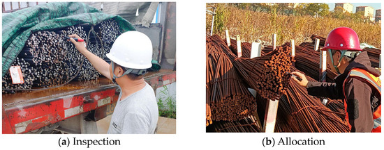
Figure 1.
Manual counting of rebars.
To date, image processing has been widely adopted in material counting on construction sites. For example, Zhang et al. [7] proposed an online counting and automatic separation system based on template matching and mutative threshold segmentation. However, this method required auxiliary light sources from appropriate angles when capturing images, limiting its application to controlled lighting environments, such as factories. Ying et al. [8] combined edge detectors and image processing algorithms to separate rebars from the background and adopted an improved Hough transform to localize them. Zhao et al. [9] used improved edge detection, image processing, and edge clustering algorithms to detect the number of rebars, but their approach required a stable detection environment. Su et al. [10] adopted an improved gradient Hough circle transform combined with the radius captured by a maximum inscribed circle algorithm to localize rebars in captured images. Wu et al. [11] proposed an online rebar counting method utilizing concave dot matching for segmentation, K-level fault tolerance for counting, and visual feedback for multiple splitting. Liu et al. [12] combined the Canny operator with a morphological edge enhancement algorithm to extract the region of interest and remove noise for automatic counting of circular steel pipes.
The core concept of the above image-processing-based counting methods has been to segment each bar in the image. These approaches have strict requirements in terms of the lighting conditions, material section, and background. However, images captured on construction sites often include various interference factors, such as uneven indentations, oxidation, corrosion, occlusions on bar ends, and nonuniform lighting, that make image-processing-based methods impractical. Additionally, little research has been conducted on counting square steel tubes because the human process of stacking square tubes sometimes results in random rotation, which makes image processing for them more challenging than that for rebars and pipes. Figure 2 shows the random rotation of square tubes in sparse and dense arrangement scenarios.
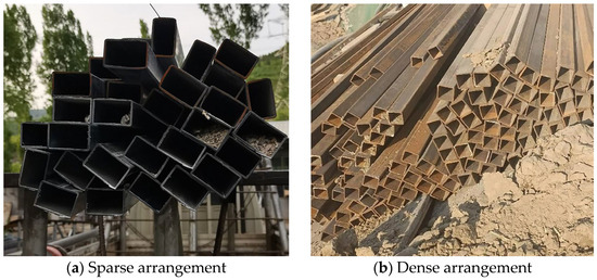
Figure 2.
Random rotations of square tubes.
Recently, deep learning has attracted significant attention and has been applied in various areas of civil engineering. By combining simple nonlinear modules, deep learning achieves highly complex functions with stronger feature extraction and generalization capabilities than traditional machine learning methods, enabling the identification of complex contents in massive datasets [13]. Among many deep learning networks that have been proposed, convolutional neural networks offer significant advantages for image processing. Object detection algorithms based on deep learning can rapidly and accurately determine the positions and categories of objects in images [14]. Currently, object detection frameworks based on deep learning can be divided into one-stage detectors and two-stage detectors [15]. One-stage detectors are more time-efficient without a significant decrease in accuracy and more suitable for real-time detection than two-stage detectors [16]. Furthermore, in one-stage detectors, the YOLOv4 [17] algorithm has been widely applied to solve problems in civil engineering owing to its excellent performance [18,19,20]. This study proposes a new counting method based on an improved YOLOv4 model to count square tubes on construction sites in real time that can be extended to address counting issues of rebars, circular pipes, and I-beams. The proposed method was subsequently applied by developing a mobile application and a WeChat mini-program for practical use on construction sites.
The remainder of this paper is organized as follows. Section 2 introduces an image dataset of steel materials and evaluation metrics. Section 3 explains the square tube counting model and the proposed improvements to the original YOLOv4 model. Section 4 interprets several training strategies and their implementation. Section 5 presents testing results and extensions of the counting method. Section 6 illustrates the deployment of the counting models to mobile devices. Conclusions are presented in Section 7.
2. Dataset and Evaluation Metrics
2.1. Steel Cross-Section Image Dataset
Object detection based on deep learning is a typical data-driven method that requires numerous real samples for training and evaluation. Conventional horizontal object detection is discouraged when objects are exhibited in arbitrary directions [21]. Instead, oriented bounding boxes can effectively detect objects with arbitrary orientations and cluttered arrangements [22] and compactly enclose each object [23]. Oriented object detection has been applied in remote sensing [24], autonomous driving [25], and power grid maintenance [26]. Therefore, this study adopts oriented object detection to count square tubes. In this study, cross-section images of square tubes at actual construction sites were captured using a typical smartphone camera. The dataset consists of 602 images and 71,887 square tube instances. The annotation tool roLabelImg v3.0 was used to assign the rotating rectangular ground-truth bounding boxes to the cross-sections of the square tubes, and the center coordinates, dimensions, widths, and angles of all cross-sections were saved in the corresponding XML annotation files, as shown in Figure 3.

Figure 3.
A raw image with annotations and an annotation file.
To further promote the development and evaluation of intelligent counting methods, datasets of other steel materials such as rebars, circular pipes, and I-beams were also established in this study. Figure 4 shows several representative images of these steel materials with annotations. Images of rebars and circular pipes were manually annotated with rectangular ground-truth bounding boxes, and images of I-beams were annotated with polygon ground-truth bounding boxes.
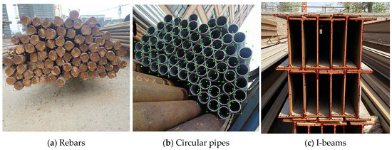
Figure 4.
Representative images with annotations.
As listed in Table 1, the final dataset used in this study comprised 991 images of rebars, 1019 images of circular pipes, 602 images of square tubes, and 501 images of I-beams. The total instances of rebars, circular pipes, square tubes, and I-beams were 181,375, 154,044, 71,887, and 18,578, respectively.

Table 1.
Details of steel material datasets.
Anchor boxes are conducive to accelerating model training and improving detection accuracy. k-means clustering was applied to obtain anchor boxes of each type of steel material using ground-truth boxes in the corresponding dataset. The results are shown in Table 1 and Figure 5. Data points with the same color belong to the same cluster, and the red stars represent anchor boxes.
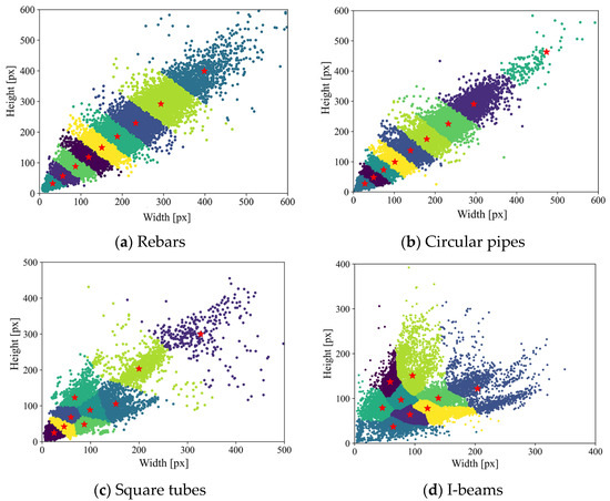
Figure 5.
Steel object clustering results.
2.2. Evaluation Metrics
Average precision (AP) [27] is a commonly used metric used to evaluate object detection model performance. However, the use of a single metric is unsuitable for the intelligent object counting model developed in this study because AP is a comprehensive metric that includes both localization and counting information, making it difficult to separate the impacts of these two factors. The mean absolute error (MAE) [28] and root-mean-square error (RMSE) [29] are useful as evaluation metrics for counting. The MAE and RMSE metrics only include counting information and may lead to false positives, in which the model correctly counts a certain number of the intended identification target but mistakenly counts other objects as targets. Therefore, this study comprehensively adopted the AP, MAE, and RMSE metrics. The AP metric is defined as follows:
where r represents the recall value, n represents the number of interpolated points, and represents the precision at the recall of . This study used AP50, which refers to an intersection over union (IoU) threshold of 0.5, to evaluate the detection performance of the model.
The MAE is used to evaluate the counting accuracy of the model, whereas RMSE is used to evaluate the counting robustness of the model. The RMSE metric assigns greater weights to larger errors and is more susceptible to outliers. Hence, this metric is used to measure the counting robustness. The MAE and RMSE metrics are calculated as
where n represents the number of images in the test set, is the actual number of instances in the image, and is the number of detections.
3. Square Tube Counting Model and Improvements
3.1. Square Tube Counting Model
As mentioned in Section 2.1, the random rotation of square tubes may cause shape orientation changes, making them difficult to detect. Figure 6 shows the differences between square tube detection and circular pipe detection: the overlapping areas and cluttered regions of bounding boxes of square tubes are larger than those of circular pipes. Larger overlapping areas result in the abandonment of certain objects after non-maximum suppression. Furthermore, cluttered regions introduce a great deal of noise, causing interference or even the disappearance of image information features.
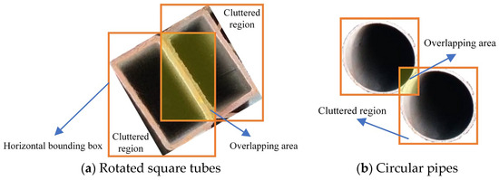
Figure 6.
Horizontal bounding boxes for detecting square tubes and circular pipes.
Therefore, this study proposed an improved YOLOv4 method for square tube counting. The establishment of the counting model adopting oriented object detection is discussed in detail below.
3.2. Improvements in Network Architecture
For object detection tasks in computer vision, once an object is associated with a specific feature map, the corresponding positions in other feature maps are considered the background. This leads to conflicts and interference during feature extraction, reducing the effectiveness of the model. To address this issue, an attention mechanism is typically applied to focus the network on essential features, thereby improving model accuracy. Adaptive spatial feature fusion (ASFF) [30] can fuse feature maps of different resolutions into a fixed-resolution feature map, reducing the inconsistency between differently scaled features caused by the correlation between large objects and low-resolution feature maps, as well as between small objects and high-resolution feature maps. Therefore, ASFF was adopted in this study to directly select and combine effective information from different resolutions, thereby enhancing model performance. The performance of different attention mechanisms was compared through experiments. The model performed best using the squeeze and excitation (SE) module [31] in combination with ASFF. The final overall network architecture is shown in Figure 7, the SE model is depicted in Figure 8, and the ASFF is described in Figure 9.
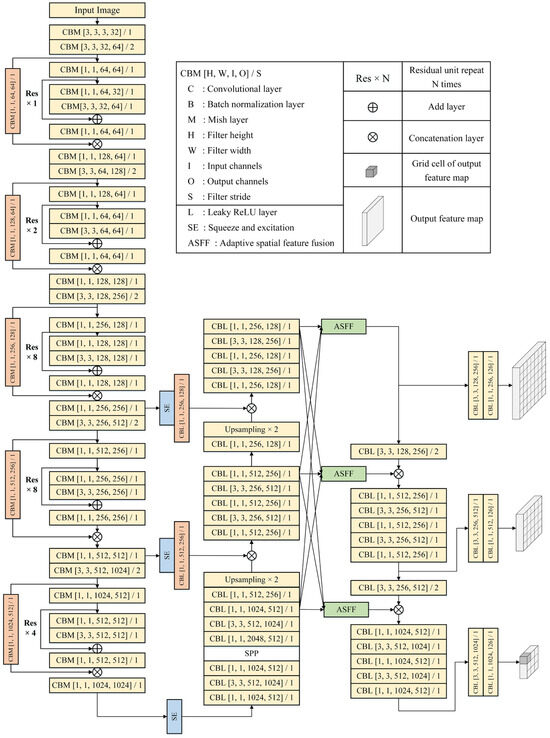
Figure 7.
Network of the square tube counting model.
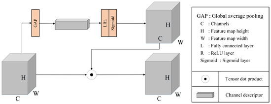
Figure 8.
Network of the SE module.
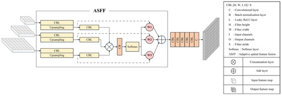
Figure 9.
Network of the ASFF module.
3.3. Improvements to the Loss Function
The original YOLOv4 model divides the output feature map into different grid cells. Each grid cell predicts three bounding boxes containing coordinates, confidence scores, and class information. The complete intersection over union (CIoU) loss is used to calculate the localization loss [32] by considering the overlapping area of the target boxes, center distance, and aspect ratio in the bounding box regression and is defined as
where LCIoU represents the CIoU loss; bp and bg represent the center points of the predicted bounding box (the gray shaded area) and the ground-truth box (the blue shaded area), respectively; dc represents the distance between bp and bg; de represents the diagonal length of the smallest box (the red dotted rectangle) enclosing the two boxes; v represents the consistency of the aspect ratio; and (wg, hg) and (wp, hp) represent the (width, height) of the predicted bounding box and ground-truth box, respectively, as shown in Figure 10.
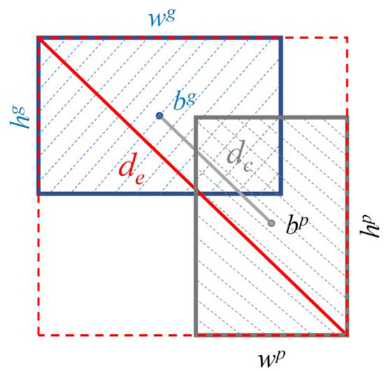
Figure 10.
Schematic of the CIoU loss.
As the CIoU loss function does not include angle information, to perform regression on rotated bounding boxes, the angle of the rotation must be defined and applied using a new localization loss function. In a two-dimensional Cartesian coordinate system, rotated rectangular bounding boxes are typically defined by the OpenCV definition method or the long-edge definition method [33]. The OpenCV definition method defines the edge that forms an acute angle with the x-axis as the box width with an angle range of [−90°, 0°], as shown in Figure 11a. The long-edge definition method defines the longer edge as the box width, with an angle range of [−90°, 90°], as shown in Figure 11b. As the descriptions of parameters in the long-edge definition method are clearer than those in the OpenCV definition method, the long-edge definition method was adopted in this study.
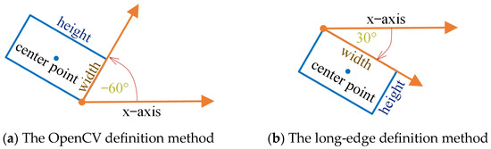
Figure 11.
Different definition methods for rotated rectangular bounding boxes.
The localization loss function was used to measure the difference between the predicted bounding box and the ground-truth box. In this specific implementation, the parameters of the rotated bounding box were converted into Gaussian distribution features comprising the mean and variance. The Kullback–Leibler (KL) divergence [34] and Gaussian Wasserstein Distance (GWD) [35] were used to quantify the difference between the two two-dimensional Gaussian distributions as the localization loss in the proposed counting model. As shown in Figure 12, the defined parameters of the rotated bounding box can be converted into Gaussian distribution features as follows:
where R represents the rotation matrix; S represents the diagonal matrix of the eigenvalues; μ and σ represent the mean vector and covariance matrix, respectively, of the two-dimensional Gaussian distribution; and x, y, w, h, and θ represent the horizontal and vertical coordinates, width, height, and angle of the rotated box, respectively. This transformation method effectively solves the issues of loss discontinuity caused by the periodicity of angles and boundary discontinuity caused by the interchange of the long and short sides [34].
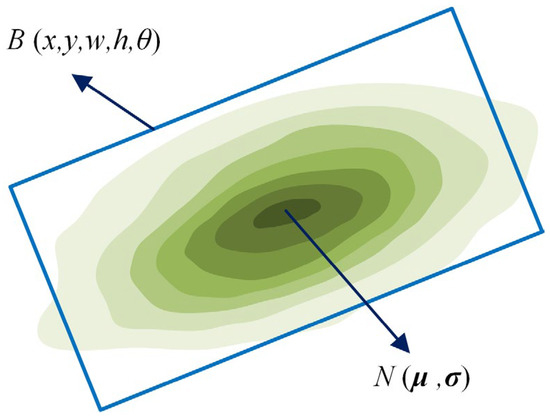
Figure 12.
Modeling a rotating bounding box using a two-dimensional Gaussian distribution.
After transforming the two-dimensional Gaussian distribution, the losses corresponding to the KL divergence and GWD were calculated as
where Dkl and Dgw represent the KL divergence and GWD, respectively; N(μ, σ) represents the two-dimensional normal distribution; μ and σ represent the mean vector and covariance matrix, respectively, of the corresponding distribution; subscripts p and t represent the predicted bounding box and ground-truth box, respectively; Tr represents the trace of a matrix; denotes the Euclidean norm of a vector; losskl and lossgw represent the loss functions based on KL divergence and GWD, respectively; and τ is a tunable parameter, which was set to two in this study.
The original YOLOv4 model has three horizontal anchor boxes, making it difficult to fit the rotated ground-truth boxes of square tubes and leading to a decrease in detection accuracy. This issue was addressed in this study by augmenting each anchor box with six additional angles {−60°, −30°, 0°, 30°, 60°, 90°}, resulting in 18 anchor boxes at each grid on the feature map. Although this approach increases the thickness of the network detection head, it also effectively improves the detection accuracy of the model.
In addition, the positive and negative samples from all the anchor boxes were differentiated during model training. A positive sample at each grid must have an IoU for the corresponding ground-truth box that is greater than a certain threshold. It must also have the highest IoU value among all the anchor boxes at that grid. While calculating the IoU for horizontal object detection is simple and fast, calculating the IoU between rotated bounding boxes during the training phase is more time-consuming. Therefore, an approximate IoU, called the ArIoU, was used to calculate the IoU during the training phase as follows:
where T represents the ground-truth box; A represents the anchor box; θT and θA, respectively, represent the angles of the ground-truth box and anchor box; and A* represents anchor box A with the angle adjusted to θT. The definition of positive samples was modified as follows:
where 1 represents a positive sample; 0 represents a negative sample; and α, β, and γ are the adjustable parameters that were, respectively, set to 0.6, 0.4, and 15° in this paper.
The original YOLOv4 model used binary cross-entropy loss as the confidence function during training. To reduce the impact of the foreground–background class imbalance on model training and enhance the sensitivity of the model to difficult samples, the original confidence function was replaced with focal loss (FL) [36], which is defined as
where Lconf is the confidence loss with FL; y and y′ represent the ground-truth and predicted values of confidence, respectively; and the adjustable parameter δ is used to balance the importance of easy and difficult samples. During the training process, the FL automatically reduces the contribution of easy background examples to the training weights and rapidly focuses on learning difficult negative samples. The focus parameter, δ, was set to two for all experiments in this study.
4. Model Training Strategy Selection and Implementation
Different deep learning models adopt different training strategies, and an effective training strategy can significantly improve the detection performance of a model. Commonly used training strategies include data augmentation, learning rate schedules, transfer learning, and multi-scale training.
4.1. Data Augmentation
The purpose of data augmentation is to enhance the original image and enrich the training dataset, making the resulting model more robust for different images. Geometric and photometric distortions are two commonly used augmentations. The flip, translation, and rotation are used in geometric distortions. The brightness, contrast, and saturation are used in photometric distortions. Figure 13 shows the augmentation effect of geometric distortions. Because the number of collected images of square tubes in this study was limited, and such objects can be placed at various angles in actual scenarios, rotation was applied for data augmentation to help the model learn to detect square tubes at many different angles using only limited data, thereby improving its generalization ability. In this study, random geometric transformations were applied to half the images in the dataset before model training, followed by random photometric transformations.
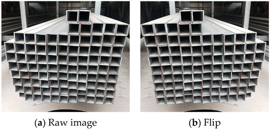
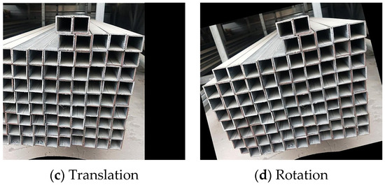
Figure 13.
Schematic views of data augmentation.
4.2. Learning Rate Schedule
The learning rate is a hyperparameter that controls the magnitude of the gradient update during the training. An optimal learning rate not only ensures the convergence of the model but also improves its training efficiency. Therefore, an appropriate learning rate schedule should be devised for the training process. This study adopted cosine annealing [37] with warmup [38] for the learning rate schedule as follows:
where ηmax and ηmin represent the maximum and minimum values of the learning rate, respectively; ηt is the learning rate of the current epoch; Tcur represents the current epoch of the training phase; Twarm represents the total epochs of the warmup phase; and Ttotal represents the total epochs of the training phase. In this study, the maximum and minimum learning rates were set to 0.0002 and 0, respectively. The total training epoch was set to 120. When using cosine annealing with warmup, the epochs of the warmup and cosine annealing were set to 12 and 108, respectively. The Adam optimizer was applied to update parameters. The batch size was set to six, and the Mish function was adopted in the activation layer. Figure 14 depicts the evolution of the learning rate over time using different learning rate schedules.
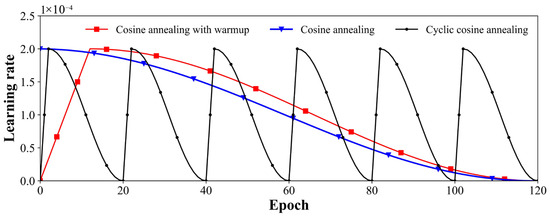
Figure 14.
Learning rate schedules.
Table 2 lists the AP values of the counting model using different learning rate schedules. The results indicate that the cosine annealing with warmup provided the highest AP value.
Table 2.
AP values of models using different learning rate schedules.
4.3. Transfer Learning
The ideal scenario for traditional machine learning involves abundant labeled training data with the same distribution as the test dataset. However, in many scenarios, collecting sufficient training data is expensive, time-consuming, or impractical. Transfer learning, which extracts useful features from a task in one domain and applies them to a new task, represents a promising strategy for solving such problems. Directly training deep learning models without using transfer learning often results in suboptimal performance. Therefore, this study attempted to use the pre-trained weights from the MS-COCO dataset [40] for weight initialization when training the square tube counting model.
However, the test results obtained by the counting model were not as accurate as expected since the square tube dataset significantly differed from the COCO dataset. Furthermore, owing to the limited number of images in the square tube dataset and the significant differences between the types and shapes of square tubes, few improvements in the accuracy of the counting model were observed after retraining. Therefore, considering the features shared by circular pipes and square tubes, as well as the greater abundance of images in the circular pipe dataset, the weights trained on the circular pipe dataset were used as the initial weights for the square tube counting model.
4.4. Multi-Scale Training
Before being input into the model, the images were generally adjusted to a fixed scale. If this scale is too large, an out-of-memory error may occur, whereas, if it is too small, the training accuracy requirements may not be satisfied. Therefore, the images must be adjusted to an appropriate scale, i.e., resolution.
Empirical evidence has shown that models trained on a fixed scale exhibit poor generalization [41]. As the multi-scale training strategy has proven effective in practice [42], this study employed multi-scale training to enhance the generalization ability of the model. For every ten batches, a random scale was selected from {416, 448, 480, 512, 544, 576, 608}, and the images were adjusted to that scale for training.
5. Results and Discussion
5.1. Analysis of the Results
Table 3 compares the performance of the square tube counting model under different situations. In this experiment, 602 images of square tubes were randomly split into training and test sets in proportions of 80% and 20%, respectively. The same data augmentation and learning rate schedules were used in all models. During the model testing phase, the image input scale was set to 608, and the confidence loss was calculated using FL.
Table 3.
Testing results of different models.
The results in Table 3 indicate significant differences in accuracy when using different attention mechanisms and loss functions. The largest difference in AP was 8.21, and the largest difference in MAE was 1.05. The AP values were generally higher when GWD was used as the loss function than when KL divergence was used. By comparing the equations for the two loss functions presented in Section 3.3, the lower AP values obtained when using the KL divergence can be inferred as the result of its asymmetry, which means the KL divergence between two distributions differs from the reverse KL divergence between the same distributions. Thus, when the predicted bounding and ground-truth boxes remain the same, the loss values will change when their positions are swapped.
When the model adopted the SE attention mechanism (Figure 8), with ASFF (Figure 9) with GWD as the loss function, the highest AP value was 91.41%, and the MAE value was 4.07. These results indicate that the proposed improvements to the original YOLOv4 model presented in this study were highly effective. The detection results with and without the improved loss function are compared in Figure 15, which shows that false detections and significant errors in the sizes and angles of the detection boxes occurred before the loss function was changed.
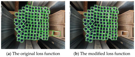
Figure 15.
Comparison of the results under different loss functions.
After modification, the counting accuracy of the model was significantly improved, and the instances of false and missed detections decreased considerably. Examples of the counting performance of the final model in two challenging scenarios (dense and scattered arrangements) are shown in Figure 16.
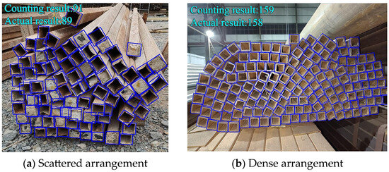
Figure 16.
Square tube counting results using the proposed counting model.
5.2. Extension of Model to Rebar, Circular Pipe, and I-Beam Counting
The approach used to establish the square tube counting model can be directly extended to rebars, circular pipes, and I-beams. As real-time counting models for individual material types have been developed separately [46,47], the modeling process is not described in detail in this paper. Examples of counting results are shown in Figure 17.
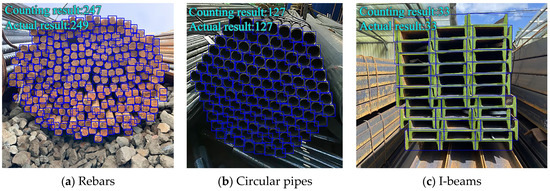
Figure 17.
Rebars, circular pipes, and I-beams counting results.
5.3. Discussion
To validate the proposed counting model, a comparison of this study and similar research was conducted. Hernández-Ruiz et al. [48] designed an SA-CNN-DC model, adopting binary classification and distance clustering to automatically count squared steel bars from images. Ghazali et al. [49] proposed a steel detection and counting algorithm adaptable to rectangular steel bars. This method utilized the Hough transform, followed by a postprocessing stage and a series of morphological operations. Comparison results are presented in Table 4.
Table 4.
Comparison results of this study and similar research.
As shown in Table 4, the accuracy of the improved YOLOv4 model was lower than the accuracies of the SA-CNN-DC model and the Hough transform model. However, there is a significant gap in the number of testing images. Additionally, the testing images in other studies were collected at a warehouse, which could provide stable lighting and a simple background. By contrast, the improved YOLOv4 model could count square tubes on construction sites and have higher robustness. The aforementioned reasons also led to a higher MAE value in the improved YOLOv4 model than in the SA-CNN-DC model. In terms of the RMSE metric, the proposed methodology demonstrated a lower value, indicating that the proposed model performed favorably. It is worth mentioning that the inference time of the improved YOLOv4 model was significantly shorter than that of the other two studies, making it suitable for real-time counting applications.
The proposed model still demonstrated suboptimal detection and counting performance in some challenging scenarios at construction sites. Moreover, counting different types of steel materials requires different detection methods, which is not practical and can be a significant drain on computing and hardware resources.
In the future, more construction sites and other building material images should be collected to include a more diverse range of images and scenarios. More contemporary detection algorithms and networks should be considered to improve the model’s performance. Additionally, a unified counting model adaptable to different kinds of steel materials should be studied and developed, ultimately enhancing its applicability in practice.
6. Counting Model Deployment
An “Intelligent Steel Counting” smartphone application was developed to practically apply the proposed counting method and address problems encountered on actual construction sites. Users of this application need only download it from a mobile application store and register to use it. The application homepage and an example of the counting results provided by the application are shown in Figure 18.
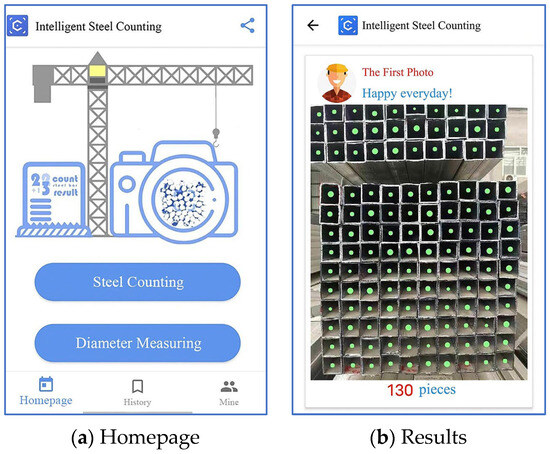
Figure 18.
Functions of the Intelligent Steel Counting smartphone application.
When using the application, users upload end-face images of steel material to the server by taking photos with smartphones to complete quantity calculations. The entire calculation and result feedback process generally takes 1–2 s, effectively meeting the requirements for real-time counting. Since its launch, this application has attracted over 28,000 registered users and has completed counting tasks for approximately 180,000 images.
In addition, a WeChat mini-program called “Intelligent Steel Counting” was developed and launched, which users can employ without downloading anything. The functions and usage of the WeChat mini-program are similar to those of the mobile application mentioned above. The homepage of the WeChat mini-program is shown in Figure 19 and Figure 20 shows examples of its counting results.
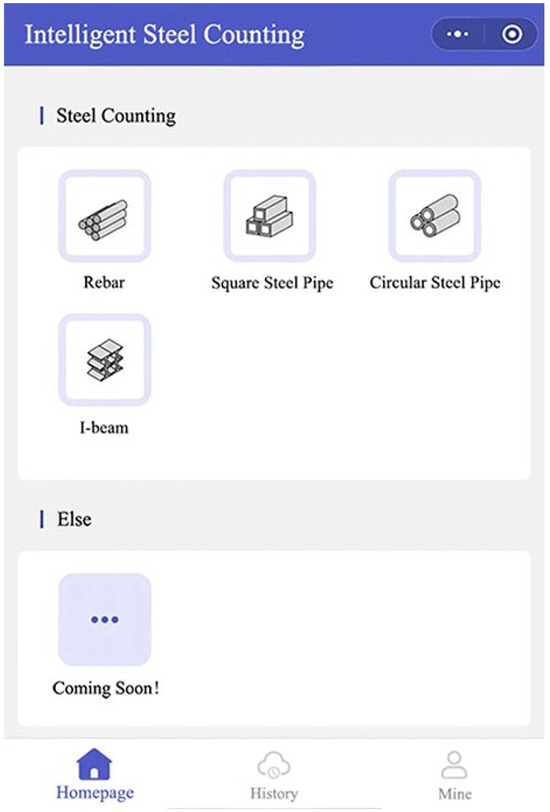
Figure 19.
Homepage of the Intelligent Steel Counting WeChat mini-program.
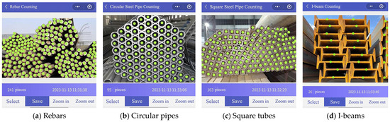
Figure 20.
Results provided by the Intelligent Steel Counting WeChat mini-program.
7. Conclusions
This study proposed an intelligent counting method for different steel materials on construction sites and developed a practical mobile application and a WeChat mini-program to minimize manual counting. The following conclusions were drawn from the results.
- To count square tubes at different angles, this study adopted oriented object detection, which can compactly enclose each object, instead of horizontal object detection.
- This study incorporated the SE attention mechanism, the ASFF module, and a loss function specifically designed for angled objects into the YOLOv4 model to improve the performance of the square tube counting model. Furthermore, the accuracy of the model was significantly improved by combining strategies, including data augmentation and learning rate schedules. In ordinary scenarios, the square tube counting model achieved an AP of greater than 90% and an MAE of 4.07.
- The research findings were implemented in a practical mobile application and a WeChat mini-program that have gained a significant user base as they can reduce the need for manpower and resources in actual construction projects.
Notably, this study was subject to several limitations. Owing to the limited training data, the counting capabilities of the square tube model require improvement in complex visual scenarios. Although the intelligent real-time counting of major steel materials in construction was achieved, new models are required to count other related materials, such as scaffolding couplers, templates, and blocks. A unified model for counting different components should be investigated in the future to further promote practicality.
Author Contributions
Conceptualization, J.C. and Y.L.; methodology, Q.H.; software, W.C., Y.C. and Y.L.; validation, W.C., Y.C., Q.H. and Y.L.; formal analysis, W.C. and Q.H.; investigation, W.C., Y.C. and Y.L.; writing—original draft preparation, Q.H.; writing—review and editing, J.C. and Y.L.; supervision, J.C. and Y.L.; funding acquisition, J.C. All authors have read and agreed to the published version of the manuscript.
Funding
This research was funded by the National Natural Science Foundation of China (Grant No. 52178151) and Tongji University Cross-Discipline Joint Program (2022-3-YB-06).
Data Availability Statement
Some or all data, models, or codes supporting the findings of this study are available from the corresponding authors upon reasonable request. The datasets are available online at https://github.com/H518123 after the paper is published.
Conflicts of Interest
Author Yang Li was employed by the company China United Engineering Co., Ltd. The remaining authors declare that the research was conducted in the absence of any commercial or financial relationships that could be construed as a potential conflict of interest.
References
- Guo, H.; Lin, J.-R.; Yu, Y. Intelligent and computer technologies’ application in construction. Buildings 2023, 13, 641. [Google Scholar] [CrossRef]
- Sun, X.; Sun, Z.; Xue, X.; Wang, L.; Liu, C. Research on interactive relationships between collaborative innovation stakeholders of intelligent construction technology. China Civ. Eng. J. 2022, 55, 108–117. [Google Scholar]
- Abioye, S.O.; Oyedele, L.O.; Akanbi, L.; Ajayi, A.; Davila-Delgado, J.M.; Bilal, M.; Akinade, O.O.; Ahmed, A. Artificial intelligence in the construction industry: A review of present status, opportunities and future challenges. J. Build. Eng. 2021, 44, 103299. [Google Scholar] [CrossRef]
- Liao, Y. Speed up the transformation of the construction industry and promote high quality development: Interpretation of the guidance on promoting the coordinated development of intelligent construction and construction industrialization. Constr. Archit. 2020, 17, 24–25. [Google Scholar]
- Lou, P.; Liu, Q.; Zhou, Z.; Wang, H. Agile supply chain management over the internet of things. In Proceedings of the International Conference on Management and Service Science, Wuhan, China, 12–14 August 2011; pp. 1–4. [Google Scholar]
- Zhang, G.; Shang, X.; Alawneh, F.; Yang, Y.; Nishi, T. Integrated production planning and warehouse storage assignment problem: An IoT assisted case. Int. J. Prod. Econ. 2021, 234, 108058. [Google Scholar] [CrossRef]
- Zhang, D.; Xie, Z.; Wang, C. Bar section image enhancement and positioning method in on-line steel bar counting and automatic separating system. In Proceedings of the IEEE Conference on 2008 Congress on Image and Signal Processing (CISP), Sanya, China, 27–30 May 2008; pp. 319–323. [Google Scholar] [CrossRef]
- Ying, X.; Wei, X.; Pei-xin, Y.; Qing-da, H.; Chang-hai, C. Research on an automatic counting method for steel bars’ image. In Proceedings of the IEEE Conference on 2010 International Conference on Electrical and Control Engineering (ICECE), Wuhan, China, 25–27 June 2010; pp. 1644–1647. [Google Scholar] [CrossRef]
- Zhao, J.; Xia, X.; Wang, H.; Kong, S. Design of real-time steel bars recognition system based on machine vision. In Proceedings of the 2016 8th International Conference on Intelligent Human-Machine Systems and Cybernetics (IHMSC), Hangzhou, China, 27–28 August 2016; pp. 505–509. [Google Scholar] [CrossRef]
- Su, Z.; Fang, K.; Peng, Z.; Feng, Z. Rebar automatically counting on the product line. In Proceedings of the 2010 IEEE International Conference on Progress in Informatics and Computing, Shanghai, China, 10–12 December 2010; pp. 756–760. [Google Scholar] [CrossRef]
- Wu, Y.; Zhou, X.; Zhang, Y. Steel bars counting and splitting method based on machine vision. In Proceedings of the 2015 IEEE International Conference on Cyber Technology in Automation, Control, and Intelligent Systems (CYBER), Shenyang, China, 8–12 June 2015; pp. 420–425. [Google Scholar] [CrossRef]
- Liu, Y.; Liu, Y.; Sun, Z. Research on stainless steel pipes auto-count algorithm based on image processing. In Proceedings of the 2012 Spring Congress on Engineering and Technology, Xi’an, China, 27–30 May 2012; pp. 1–3. [Google Scholar] [CrossRef]
- LeCun, Y.; Bengio, Y.; Hinton, G. Deep learning. Nature 2015, 521, 436–444. [Google Scholar] [CrossRef]
- Zhao, Z.-Q.; Zheng, P.; Xu, S.; Wu, X. Object detection with deep learning: A review. IEEE Trans. Neural Netw. Learn. Syst. 2019, 30, 3212–3232. [Google Scholar] [CrossRef]
- Wu, X.; Sahoo, D.; Hoi, S.C.H. Recent advances in deep learning for object detection. Neurocomputing 2020, 396, 39–64. [Google Scholar] [CrossRef]
- Xiao, Y.; Tian, Z.; Yu, J.; Zhang, Y.; Liu, S.; Du, S.; Lan, X. A review of object detection based on deep learning. Multimed. Tools Appl. 2020, 79, 23729–23791. [Google Scholar] [CrossRef]
- Bochkovskiy, A.; Wang, C.-Y.; Liao, H.-Y.M. YOLOv4: Optimal speed and accuracy of object detection. arXiv 2020, arXiv:2004.10934. [Google Scholar] [CrossRef]
- Wu, P.; Liu, A.; Fu, J.; Ye, X.; Zhao, Y. Autonomous surface crack identification of concrete structures based on an improved one-stage object detection algorithm. Eng. Struct. 2022, 272, 114962. [Google Scholar] [CrossRef]
- Xu, L.; Fu, K.; Ma, T.; Tang, F.; Fan, J. Automatic detection of urban pavement distress and dropped objects with a comprehensive dataset collected via smartphone. Buildings 2024, 14, 1546. [Google Scholar] [CrossRef]
- Yu, Z.; Shen, Y.; Shen, C. A real-time detection approach for bridge cracks based on YOLOv4-FPM. Autom. Constr. 2021, 122, 103514. [Google Scholar] [CrossRef]
- Yao, Y.; Cheng, G.; Wang, G.; Li, S.; Zhou, P.; Xie, X.; Han, J. On improving bounding box representations for oriented object detection. IEEE Trans. Geosci. Remote Sens. 2023, 61, 5600111. [Google Scholar] [CrossRef]
- Dai, L.; Liu, H.; Tang, H.; Wu, Z.; Song, P. AO2-DETR: Arbitrary-oriented object detection transformer. IEEE Trans. Circuits Syst. Video Technol. 2023, 33, 2342–2356. [Google Scholar] [CrossRef]
- Ma, J.; Shao, W.; Ye, H.; Wang, L.; Wang, H.; Zheng, Y.; Xue, X. Arbitrary-oriented scene text detection via rotation proposals. IEEE Trans. Multimed. 2018, 20, 3111–3122. [Google Scholar] [CrossRef]
- Huang, Z.; Li, W.; Xia, X.-G.; Wang, H.; Tao, R. Task-wise sampling convolutions for arbitrary-oriented object detection in aerial images. IEEE Trans. Neural Netw. Learn. Syst. 2024, 1–15. [Google Scholar] [CrossRef]
- Park, H.-M.; Park, J.-H. Multi-lane recognition using the YOLO network with rotatable bounding boxes. J. Soc. Inf. Disp. 2023, 31, 133–142. [Google Scholar] [CrossRef]
- Wu, J.; Su, L.; Lin, Z.; Chen, Y.; Ji, J.; Li, T. Object detection of flexible objects with arbitrary orientation based on rotation-adaptive YOLOv5. Sensors 2023, 23, 4925. [Google Scholar] [CrossRef]
- Everingham, M.; Van Gool, L.; Williams, C.K.I.; Winn, J.; Zisserman, A. The PASCAL visual object classes (VOC) challenge. Int. J. Comput. Vis. 2010, 88, 303–338. [Google Scholar] [CrossRef]
- Willmott, C.J.; Matsuura, K. Advantages of the mean absolute error (MAE) over the root mean square error (RMSE) in assessing average model performance. Clim. Res. 2005, 30, 79–82. [Google Scholar] [CrossRef]
- Jackson, E.K.; Roberts, W.; Nelsen, B.; Williams, G.P.; Nelson, E.J.; Ames, D.P. Introductory overview: Error metrics for hydrologic modelling—A review of common practices and an open source library to facilitate use and adoption. Environ. Modell. Softw. 2019, 119, 32–48. [Google Scholar] [CrossRef]
- Liu, S.; Huang, D.; Wang, Y. Learning spatial fusion for single-shot object detection. arXiv 2019, arXiv:1911.09516. [Google Scholar] [CrossRef]
- Hu, J.; Shen, L.; Sun, G. Squeeze-and-excitation networks. In Proceedings of the 2018 IEEE Conference on Computer Vision and Pattern Recognition, Salt Lake City, UT, USA, 18–22 June 2018; pp. 7132–7141. [Google Scholar] [CrossRef]
- Zheng, Z.; Wang, P.; Liu, W.; Li, J.; Ye, R.; Ren, D. Distance-IoU loss: Faster and better learning for bounding box regression. In Proceedings of the 34th AAAI Conference on Artificial Intelligence, New York, NY, USA, 7–12 February 2020; Volume 34, pp. 12993–13000. [Google Scholar] [CrossRef]
- Yang, X.; Yan, J. On the arbitrary-oriented object detection: Classification based approaches revisited. Int. J. Comput. Vis. 2020, 130, 1340–1365. [Google Scholar] [CrossRef]
- Yang, X.; Yang, X.; Yang, J.; Ming, Q.; Wang, W.; Tian, Q.; Yan, J. Learning high-precision bounding box for rotated object detection via Kullback-Leibler divergence. In Proceedings of the 35th Conference on Neural Information Processing Systems (NeurIPS), Online, 6–14 December 2021; Volume 34, pp. 18381–18394. [Google Scholar]
- Yang, X.; Yan, J.; Ming, Q.; Wang, W.; Zhang, X.; Tian, Q. Rethinking rotated object detection with Gaussian Wasserstein distance loss. In Proceedings of the International Conference on Machine Learning (ICML), Online, 18–24 July 2021; pp. 11830–11841. [Google Scholar] [CrossRef]
- Lin, T.-Y.; Goyal, P.; Girshick, R.; He, K.; Dollar, P. Focal loss for dense object detection. In Proceedings of the 2017 IEEE International Conference on Computer Vision (ICCV), Venice, Italy, 22–29 October 2017; pp. 2999–3007. [Google Scholar] [CrossRef]
- Loshchilov, I.; Hutter, F. SGDR: Stochastic gradient descent with warm restarts. arXiv 2017, arXiv:1608.03983. [Google Scholar] [CrossRef]
- Goyal, P.; Dollár, P.; Girshick, R.; Noordhuis, P.; Wesolowski, L.; Kyrola, A.; Tulloch, A.; Jia, Y.; He, K. Accurate, large minibatch SGD: Training imageNet in 1 hour. arXiv 2018, arXiv:1706.02677. [Google Scholar] [CrossRef]
- Huang, G.; Li, Y.; Pleiss, G.; Liu, Z.; Hopcroft, J.E.; Weinberger, K.Q. Snapshot ensembles: Train 1, get M for free. arXiv 2017, arXiv:1704.00109. [Google Scholar]
- Lin, T.-Y.; Maire, M.; Belongie, S.; Hays, J.; Perona, P.; Ramanan, D.; Dollár, P.; Zitnick, C.L. Microsoft COCO: Common objects in context. In Proceedings of the 13th European Conference on Computer Vision (ECCV), Zurich, Switzerland, 6–12 September 2014; Volume 8693, pp. 740–755. [Google Scholar] [CrossRef]
- He, K.; Zhang, X.; Ren, S.; Sun, J. Spatial pyramid pooling in deep convolutional networks for visual recognition. IEEE Trans. Pattern Anal. Mach. Intell. 2015, 37, 1904–1916. [Google Scholar] [CrossRef]
- Redmon, J.; Farhadi, A. YOLO9000: Better, faster, stronger. In Proceedings of the 2017 IEEE Conference on Computer Vision and Pattern Recognition (CVPR), Honolulu, HI, USA, 21–26 July 2017; pp. 6517–6525. [Google Scholar] [CrossRef]
- Zhang, H.; Zu, K.; Lu, J.; Zou, Y.; Meng, D. EPSANet: An efficient pyramid squeeze attention block on convolutional neural network. In Proceedings of the 16th Asian Conference on Computer Vision (ACCV), Macao, China, 4–8 December 2023; Volume 13843, pp. 541–557. [Google Scholar] [CrossRef]
- Woo, S.; Park, J.; Lee, J.-Y.; Kweon, I.S. CBAM: Convolutional block attention module. In Proceedings of the 15th European Conference on Computer Vision (ECCV), Munich, Germany, 8–14 September 2018; Volume 11211, pp. 3–19. [Google Scholar] [CrossRef]
- Misra, D.; Nalamada, T.; Arasanipalai, A.U.; Hou, Q. Rotate to attend: Convolutional triplet attention module. In Proceedings of the 2021 IEEE/CVF Winter Conference on Applications of Computer Vision (WACV), Waikoloa, HI, USA, 1–6 January 2021; pp. 3138–3147. [Google Scholar] [CrossRef]
- Li, Y.; Lu, Y.; Chen, J. A deep learning approach for real-time rebar counting on the construction site based on YOLOv3 detector. Autom. Constr. 2021, 124, 103602. [Google Scholar] [CrossRef]
- Li, Y.; Chen, J. Computer vision-based counting model for dense steel pipe on construction sites. J. Constr. Eng. Manag. 2022, 148, 04021178. [Google Scholar] [CrossRef]
- Hernández-Ruiz, A.C.; Martínez-Nieto, J.A.; Buldain-Pérez, J.D. Steel bar counting from images with machine learning. Electronics 2021, 10, 402. [Google Scholar] [CrossRef]
- Ghazali, M.F.; Wong, L.-K.; See, J. Automatic detection and counting of circular and rectangular steel bars. In Proceedings of the 9th International Conference on Robotic, Vision, Signal Processing and Power Applications (RoViSP), Penang, Malaysia, 2–3 February 2016; pp. 199–207. [Google Scholar] [CrossRef]
Disclaimer/Publisher’s Note: The statements, opinions and data contained in all publications are solely those of the individual author(s) and contributor(s) and not of MDPI and/or the editor(s). MDPI and/or the editor(s) disclaim responsibility for any injury to people or property resulting from any ideas, methods, instructions or products referred to in the content. |
© 2024 by the authors. Licensee MDPI, Basel, Switzerland. This article is an open access article distributed under the terms and conditions of the Creative Commons Attribution (CC BY) license (https://creativecommons.org/licenses/by/4.0/).