Abstract
The tunnel portal section is often in extremely weak and fragmented strata, and the deformation of the portal side and slope will affect the stability of the surrounding rock and the tunnel-supporting structure. However, the deformation characteristics and displacement development patterns of slopes in the tunnel portal section are not clear. In this paper, the multifractal characteristics and displacement prediction of the deformation sequence of the tunnel portal slope at of a weak and water-rich shallow buried tunnel adjacent to an important structure are studied in depth. Combined with the deformation characteristics of the tunnel portal slope, a suitable slope monitoring and measurement scheme is designed to analyze the deformation pattern of the tunnel portal slope. Based on the multifractal detrended fluctuation analysis (MF-DFA) method, the multifractal characteristics of the deformation monitoring sequences at each monitoring point of the tunnel portal slope are analyzed. The multifractal characteristics of displacement sequences at different monitoring points of the tunnel portal slope are consistent with the actual monitoring results. Furthermore, the Long Short-Term Memory (LSTM) model is optimized using the Particle Swarm Optimization (PSO) algorithm to predict the deformation of the tunnel portal slope. The results show that the maximum mean square error (MSE) of the horizontal displacement test set prediction results is 0.142, and the coefficient of determination (R2) is higher than 91%. The maximum value of MSE for vertical displacement test set prediction is 0.069, and the R2 are higher than 91%. The study shows that the performance of the PSO-LSTM prediction model can meet the requirements for predicting the displacement of the tunnel portal slope. Based on the MF-DFA method and PSO-LSTM prediction model, the fluctuation characteristics of the displacement value of the tunnel portal section can be accurately identified and the displacement development pattern can be effectively predicted. The conclusions of the study are of great practical significance for the safe construction of the tunnel portal section.
1. Introduction
With the implementation of China’s “The Belt and Road Initiative” strategy, more and more Chinese engineering construction enterprises have gone abroad. They have undertaken a large number of overseas highways, railroads, and other infrastructure projects, contributing to the infrastructure construction of many countries in Asia and Europe. Influenced by the terrain, most of the highway and railroad projects needed to cross a large number of mountainous areas. Therefore, tunneling occupies a very important position in the construction of high-speed infrastructure in mountainous areas [1,2,3]. Numerous influencing factors need to be considered in the design and alignment of railroads. Although the engineering community has now recognized the importance of geological conditions at the tunnel portal for construction safety, tunnel construction is still unavoidable in the case of unfavorable geological conditions such as high slope, large deflections, and shallow burials [4,5,6]. In this case, if the excavation method and auxiliary construction measures chosen for tunnel construction are unreasonable, the construction process is very prone to accidents such as roofing, collapse, lining cracking, slope instability, and landslides [7,8]. It will not only cause schedule delays and economic loss but also easily lead to casualties of construction personnel on site. Therefore, how to ensure the stability of the surrounding rock and the tunnel portal slope, and understand the safety of entering and exiting the tunnel, has become one of the important researches of many experts and scholars in the field of tunnel engineering.
Existing research shows that the main factor restricting the safe entry and exit of tunnels is the stability of the surrounding rock at the tunnel entrance [9,10]. The stability of the surrounding rock of the tunnel portal section can be divided into the stability of the side slope of the tunnel portal and the stability of the surrounding rock and lining of the excavation surface of the tunnel body. At the same time, the research shows that the two are also interacting with each other. The deformation of the uphill side of the tunnel entrance will affect the stability of the surrounding rock and supporting structure of the tunnel body, and the rock and soil disturbance caused by tunnel excavation will also affect the stability of the uphill side of the tunnel entrance [11,12,13,14]. In the theoretical study of the stability of tunnel portal rock, Aygar et al. [11] analyzed the relationship between highway tunnel stability and portal slope in Turkey using numerical simulation. Wang et al. [15,16] performed a large-scale shaking table test on a tunnel portal and developed a method for detecting dynamic damage based on the Hilbert–Huang transform. This method accurately identifies macroscopic damage in tunnel linings and portal slopes. Genis et al. [17] utilized a dynamic analysis program based on the three-dimensional finite-difference method and determined that peak accelerations exceeding 0.5 g may lead to severe damage in tunnel portal slopes and the area 20–50 m from the tunnel entrance. In addition, many researchers [18,19,20,21,22] have also emphasized the significance of tunnel portal stability in tunnel construction through various studies. In applying the theory of perimeter rock stability in tunnel portal sections, Li et al. [23,24] established a three-dimensional numerical model and proposed the use of the center diaphragm and circular reserved core soil methods to excavate shallow buried tunnels. This method effectively controls peripheral rock deformation, surface settlement, and slope stability in conditions of loose and fragmented rock. Aygar and Gokceoglu [25] highlighted the impact of opening excavation on tunnels lacking cohesive foundations. Ayoublou et al. [12] emphasized the importance of slope displacement measurements and monitoring at tunnel portals. Taromi et al. [26] investigated the collapse mechanism of water conveyance tunnel portals and presented potential solutions.
In addition, in the process of tunnel construction, it is necessary to continuously monitor the slope at the entrance [27]. Analyzing and predicting the deformation pattern of the slope during tunnel portal construction can provide technical support and theoretical guidance for the early warning of tunnel portal construction safety, which is of great significance for improving the safety of tunnel portal construction. After obtaining the original tunnel portal slope monitoring data, to further prevent the occurrence of tunnel disasters, it is necessary to analyze the deformation trend and predict the displacement development in advance [28,29,30]. The deformation monitoring data of the side and elevation slopes are usually shown as complex nonlinear and non-stationary time series. The deformation sequence is characterized by discontinuous multi-scale. Compared with the simple fractal dimension, the multifractal method describes the fractal structure through the spectral function, which can more finely characterize the volatility of the deformation sequence at different levels [31,32]. In recent years, some researchers have applied multifractals to the field of geotechnical engineering [33,34,35,36]. Therefore, the multifractal theory can be used to analyze the fluctuation characteristics of the deformation sequence of the tunnel portal slope.
Tunnel slope engineering is a complex nonlinear dynamical system, and the stability and deformation of the slope are affected by many uncertain factors [37,38]. Due to the complexity, ambiguity, and randomness of the deformation of the slope during the construction of the tunnel portal. Therefore, simple statistical methods do not apply to the complex nonlinear time series slope deformation problem [39,40]. Machine learning methods can effectively replace traditional statistical methods due to their nonlinear learning ability. Support Vector Regression and Extreme Gradient Boost are the most commonly used machine learning methods in time series prediction [41]. Compared with statistical methods, machine learning methods are more likely to capture the complexity, dynamics, and nonlinear characteristics of nonlinear time series data on slope. At present, machine learning methods have achieved certain results in the research of slope deformation prediction [42,43]. In recent years, deep learning has developed rapidly [43]. Many studies have shown that its performance is better than traditional machine learning models. Commonly used deep learning methods for time series prediction include deep neural network [44,45], convolutional neural network [46], recurrent neural network (RNN) [47], and so on. Among them, RNN models have a strong fitting ability to sequence data. Long Short-Term Memory (LSTM) solves the defects of the gradient explosion problem in traditional RNN and is the most widely used RNN model [48]. The LSTM is better than traditional RNN in fitting long sequence data and has achieved better prediction results in a large number of engineering applications [49,50,51,52]. However, when the input sequence is long, the performance of the LSTM model is still poor. Optimization algorithms of group intelligence such as particle swarm algorithm (PSO) can effectively improve the performance of the LSTM, and in recent years, some related studies have applied the PSO-LSTM model to slope deformation prediction [53].
The tunnel portal section is often in extremely weak and broken strata, and the construction of the portal and the excavation of the slope uplift will disturb the slope and the internal surrounding rock [54,55]. The self-stabilizing surrounding rock will make it difficult to form an effective bearing arch, and it is very easy to have engineering accidents such as collapses, toppling, and landslides seriously affect the construction progress and the economic benefits of the project. In Malaysia, a railroad tunnel portal section can easily form a soil slope due to shallow depth. Construction disturbance during the excavation of the tunnel portal can easily induce landslides and sidewall instability, and the safety coefficient of the slope will be greatly reduced. Therefore, during the construction of the tunnel portal section, analyzing and predicting the monitoring data of the portal side and slope can provide a basis for the dynamic design and information construction of the tunnel. It is of great practical significance to improve the stability of the tunnel side slope and ensure the safe construction of the tunnel portal section.
Therefore, this study takes the construction of a soft, water-rich, and shallow buried tunnel portal section near a high-voltage power tower in Malaysia as the engineering background. Combined with on-site monitoring and measurement, multifractal analysis, and deep learning methods, an in-depth study is carried out on the multifractal characteristics of deformation and deformation prediction of the tunnel portal slope. The main research includes the following aspects. (1) Combining the deformation characteristics of the tunnel portal slope, designing a suitable monitoring and measurement scheme, and analyzing the deformation pattern of the tunnel portal slope. Evaluate the stability of the tunnel portal slope. (2) Based on the multifractal detrended fluctuation analysis method (MF-DFA), analyze the multifractal characteristics of the deformation monitoring sequences at each monitoring point of the tunnel portal slope. Analyze the change characteristics of the displacement sequence of the slope at the tunnel entrance and compare it with the actual situation. (3) Optimize the LSTM model using the PSO algorithm to predict the deformation of the tunnel portal slope. Combined with the MF-DFA multifractal features, the PSO-LSTM model is applied to predict the displacement development of the deformation monitoring points of the slope at the entrance of the tunnel.
2. Materials and Methods
2.1. Overview of the Tunnel Project
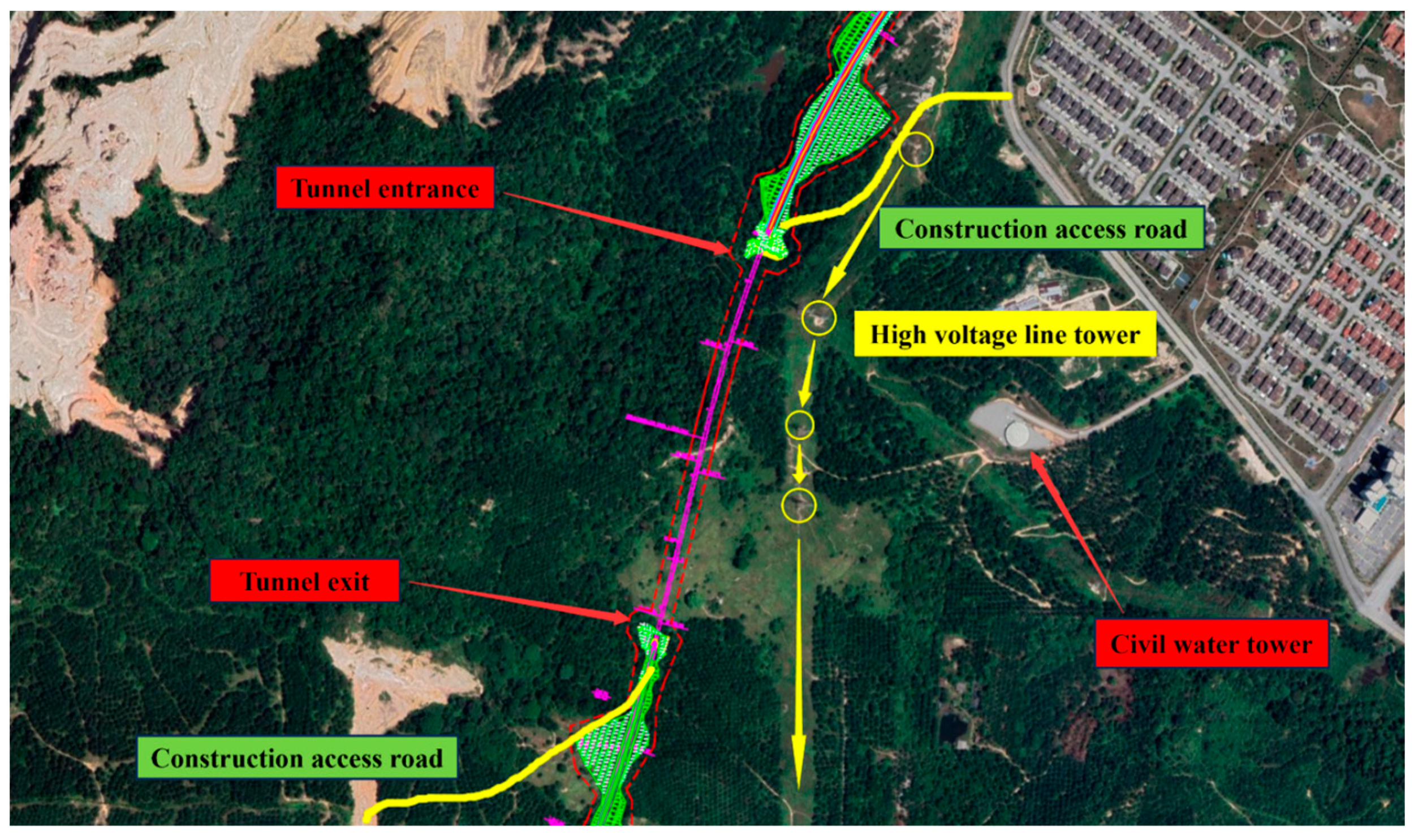
A railroad project on the east coast of Malaysia is located in Selangor State in the coastal belt of western Malaysia. The study relies on the No. 3 tunnel mileage pile number CH48 + 511~CH49 + 168, north-south direction, the total length of the tunnel is 657 m. The tunnel crosses the first peak of Cheraka Mountain, with a maximum depth of 104 m. The shallow section is 137 m long, with a maximum depth of 109 m and a minimum depth of 1.3 m. The surrounding rock is fully weathered, strongly weathered sandstone, with high mud content, and the rock body is broken. The peripheral rock of the tunnel is fully weathered and strongly weathered sandstone, with high mud content, broken rock, and local extremely broken rock. The inlet is prone to form soil slope, and the construction disturbance is prone to landslides and sidewall instability. In addition, there are two fracture zones in the tunnel, including CH48 + 537~CH48 + 580 and CH48 + 800~CH49 + 080, with a total length of about 323 m. The rock is fractured, and the fissure water is abundant, which makes the tunnel construction risk high, and there is a potential danger of landslides. Meanwhile, there are high voltage towers on the east side of the tunnel area about 140 m–200 m, and the vibration requirement for high voltage towers from the local power company in Malaysia is 3 mm/s. An aerial photo of the tunnel project route is shown in Figure 1.
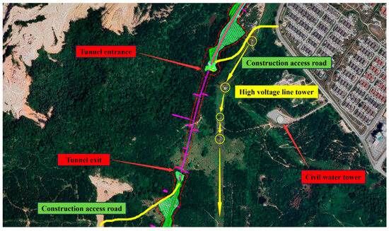
Figure 1.
The tunnel project roadmap and layout plan.
2.2. Deformation Monitoring Program for Tunnel Portal Slope
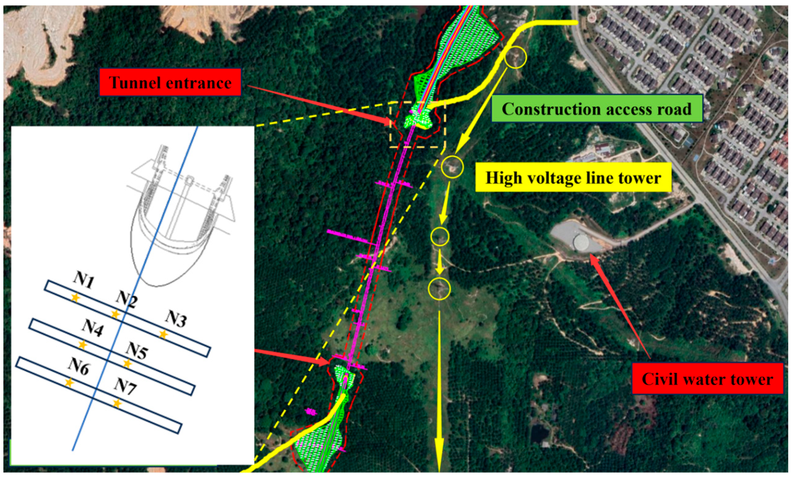
According to the ground investigation drawings, the surrounding rock at the tunnel entrance is mainly composed of fully weathered to moderately weathered residual flooding clay, fine sand, and granite, and the rock body is broken to extremely broken. Before excavation of the tunnel entrance and exit and the shallow buried section of the tunnel body, overrun pipe shed grouting support is done in strict accordance with the design. The excavation adopts the method of reserving core soil, weak blasting, or non-blasting excavation method. Into the hole, Φ108 large pipe shed combined with Φ42 small conduit for pre-protection to strengthen the initial support. At the same time, strengthen the ground surface pre-injection grouting reinforcement treatment measures, and do a good job of holes outside the anti-drainage measures. Strengthen the surface subsidence measurement during construction. The inlet section of the tunnel is a high-slope tunnel, with a large excavation volume and complicated slope protection measures. After excavation, monitoring and measuring are carried out in time, support is strengthened according to the design requirements, and the construction of back arch closure is completed in time. Before construction, the horizontal displacement and vertical settlement values of the slope at the entrance were continuously monitored. Firstly, determine the monitoring area and choose the suitable location of monitoring points. A total of 7 monitoring points are arranged on the surface of the slope at the entrance, forming 3 monitoring lines. The detailed arrangement of deformation monitoring points on the up slope of the tunnel portal side is shown in Figure 2.

Figure 2.
Arrangement of deformation monitoring points of tunnel portal slope.
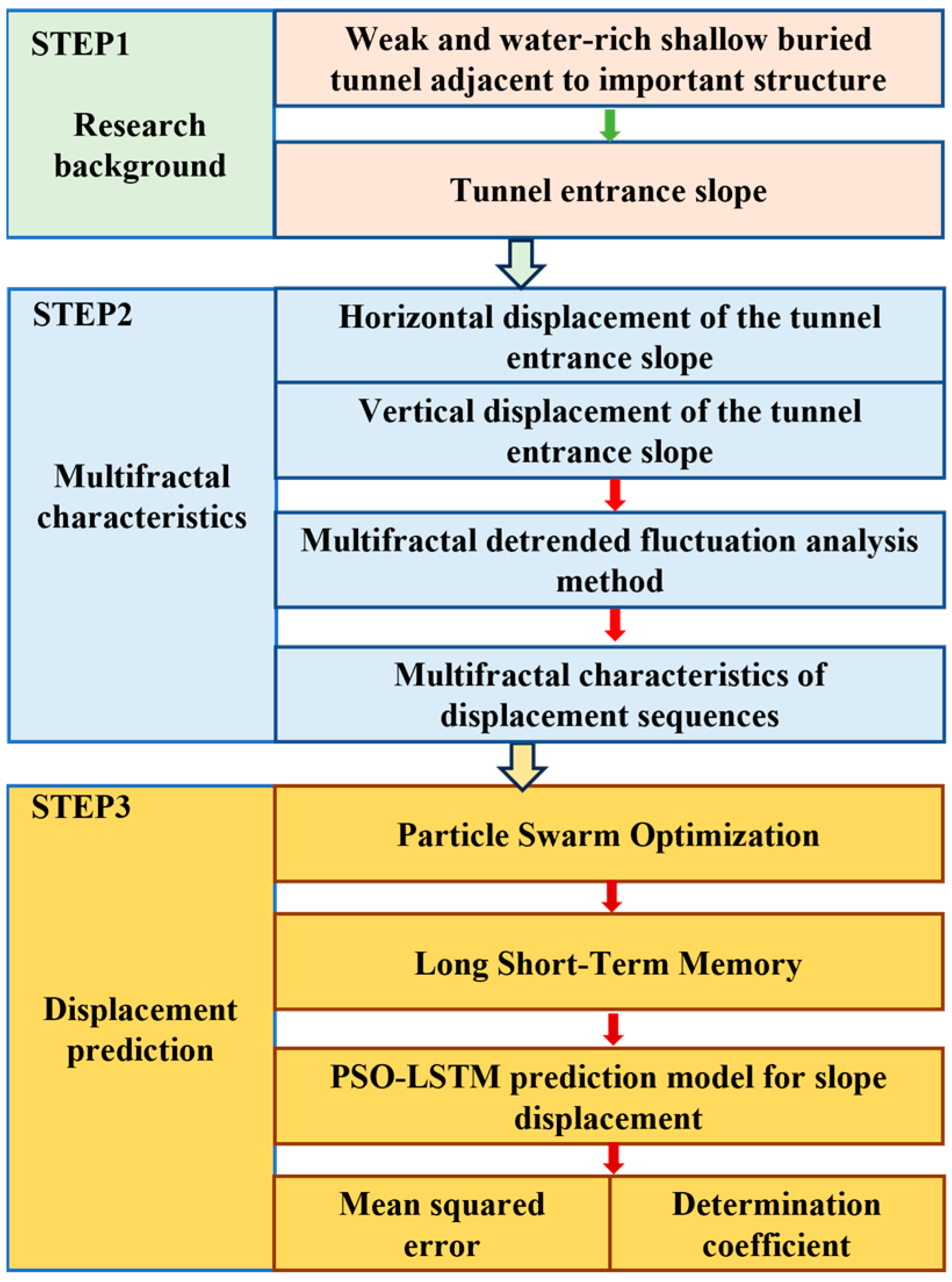
Combined with the deformation monitoring results of the tunnel portal slope, the deformation pattern of the tunnel portal slope is analyzed. Further, based on the MF-DFA method, the multifractal characteristics of the deformation sequences at each monitoring point of the slope are analyzed. The PSO-LSTM model is utilized to predict the displacement development of the deformation monitoring points. The specific flow chart of the study is shown in Figure 3.
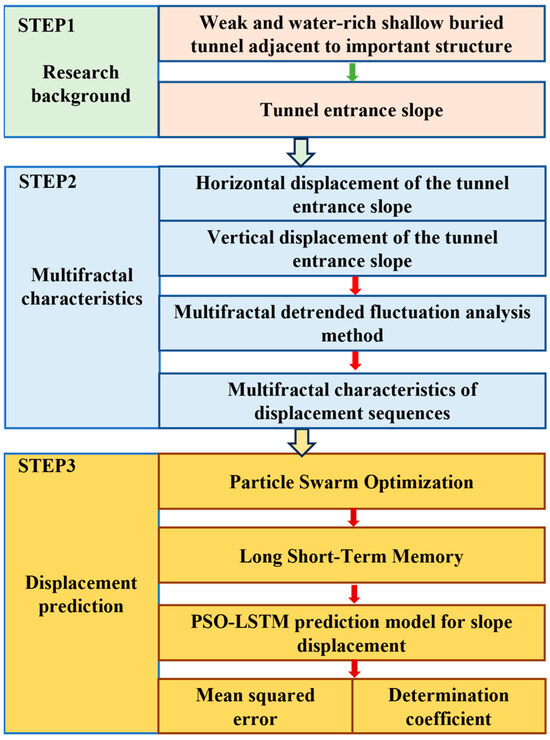
Figure 3.
Flow chart of the study.
2.3. Multifractal Detrended Fluctuation Analysis Method
MF-DFA is a method for analyzing non-stationary finite time series. MF-DFA can effectively reveal the fractal structure and nonlinear dynamic properties in the data [56,57,58]. The method combines multifractal theory and the detrended technique to reveal the complex structure and dynamic patterns of the data by analyzing the multifractal properties of the data and removing the trending components in the data. In MF-DFA, the Hurst index of the original time series is first calculated, and then the time series is divided into different sub-series according to different Hurst indices. Then, each subsequence is de-trended, i.e., the long-term trend in the subsequence is removed, and then the respective Hurst index is calculated again. By comparing the Hurst indices of the sub-series after the detrended process, the fractal characteristics in the data series can be analyzed more accurately. Specifically, the calculation of MF-DFA contains the following five steps.
Step 1: Given a time series . The length of the sequence is N and the mean value is , find the cumulative deviation sequence :
Step 2: The sequence will be equalized in terms of the time scale s.
Since N may not be an exact multiple of s, there will be leftover values in the division process . The 2m equal-length subintervals are obtained by using the reverse-order processing method.
Step 3: The corresponding residual series are obtained .
Equation: is the subinterval. denotes a kth order fitting polynomial to the vth subinterval. The variable v ranges from 1 to 2m, and t ranges from 1 to s.
Step 4: Calculate the residual sequence of the residual series .
Step 5: For the dataset, take the mean value and calculate the q-order volatility function of the series .
where q can theoretically assume any non-zero real value, and the value of q is related to the the degree of exposure to fluctuations. In particular, the MF-DFA degenerates to the standard DFA when q = 2. In particular, a limiting form of Equation (5) emerges when q = 0:
A sliding window is used to optimize the traditional MF-DFA for dividing subintervals. Let the window length be s, the sequence length be N, and the sliding step be 1.
The q-order fluctuation function for a specific scale s is derived through the aforementioned steps . Adjusting the values of s and iterating through the steps yields a series of point values. When a long-range correlation is present in this time series, a power law connection between and s is evident, as depicted in Equation (8):
Taking logarithms of the above equation yields the following form:
is the q-order volatility function of the series. The is the corresponding generalized Hurst exponent. b is the constant coefficient.
Make double logarithmic scatterplot and fit it. Its slope is the generalized Hurst exponent . If is a nonlinear subtractive function of q, then the sequence is characterized by multifractal.
The multifractal spectrum characterizing the fractal intensity and fractal singularity of a time series can typically be determined in Equations (10)–(12) as follows.
is the Renyi index, also known as the scalar function. If it is a nonlinear up-convex function of q, the sequence is characterized by multifractal. Here, represents the singular intensity, while represents the multifractal spectrum. When is a single-peak up-convex shaped like a quadratic function, it means that the sequence has multifractal characteristics.
2.4. PSO-LSTM Algorithm
2.4.1. Principles of the LSTM Algorithm
LSTM Network is a special type of Recurrent Neural Network mainly used for the task of processing and predicting sequential data. LSTM was proposed by Hochreiter and Schmidhuber in 1997 and was initially designed to solve the problem of disappearing or exploding gradients faced by conventional RNN when processing long sequential data [59]. LSTM can capture long-term dependencies through the introduction of gating mechanisms and cell states, it can maintain information over a longer period, thus capturing long-term dependencies. The main advantage of LSTM is that it can effectively handle long sequence data. The specific computational steps of LSTM are as follows:
Step 1: Data normalization. is the original data and is the normalized data.
Step 2: The LSTM model comprises multiple cells, each with specific formulas for the forgetting gate, input gate, and output gate.
where and are the results of the oblivion gate, input gate, and output gate state settlements, respectively. The is the hidden state of the moment before the time, the is the sigmoid function. , , and are the weight matrices of the forgetting gate, input gate, and output gate, respectively. , , and are the forgetting gate, input gate, and output gate bias terms, respectively.
Step 3: For the candidate value vector, the product of the input value and the candidate value vector is used to update the cell state, calculated as:
where is the input unit state weight matrix. is the input unit state bias term. is the activation function. is the neuron output value. is the current moment hidden state.
2.4.2. Principles of the PSO Algorithm
PSO is a particle swarm algorithm that simulates the foraging behavior of a flock of birds [60]. The algorithm uses the information-sharing mechanism in the biota to produce the behavior of synchronizing information between individuals and groups with each other. It is a stochastic search algorithm based on group collaboration. In the PSO algorithm, “particle” is used as an intermediate choice. Individual particles exchange information with each other, and many particles form a group to form a particle population. The objective of PSO is to facilitate numerous particles in discovering the optimal solution within a multidimensional space. This multidimensional space, often referred to as the multi-dimensional solution space, serves as the search domain for the particle swarm to locate the optimal solution. Each optimization problem corresponds to a particle within this search space. These particles are expanded into a D-dimensional space and possess a function that evaluates the quality of the particle’s current position, along with a velocity vector that dictates its movement and direction. Each iteration is a continuous search of the particles in the solution space in the direction of the current optimal particle.
The algorithm of PSO is implemented as follows: in a D-dimensional solution space, there exist N particles. Each particle possesses a velocity vector that varies in real time due to many factors. The particle velocity of the ith evolution is , with the previous velocity , the individual optimal position , and the population optimal position . The velocity update in the dth dimension of particle i is calculated as follows.
In addition, each iteration updates the position information of each particle. The position of the particle for the ith evolution is changed by the position information of the previous , and the velocity information of the previous iteration are linearly summed up. The dth dimensional position update of particle i is computed as follows.
In the optimization process, the position vector in the dth dimension of the search space fluctuates within the range of , while the velocity vector ranges within . During iterations, if the values of and exceed the boundaries, the velocity or position in that particular d-dimension is set to the maximum boundary velocity or position. Here, represents the dth dimensional component of the flight velocity searched by particle i at the kth iteration, and denotes the dth dimensional component of the position searched by particle i at the kth iteration. The parameters w, , and stand for the inertia weight (non-negative), acceleration constants, and , are random numbers within the range [0,1].
2.4.3. PSO Optimized LSTM Model
LSTM has excellent feature extraction ability for data with spatio-temporal correlation. In this study, the LSTM model is used to predict the displacement data of the tunnel portal slope. To obtain better training effects and prediction accuracy, the hyperparameters of the LSTM model need to be optimized. Since the monitoring system and monitoring data are changing in real-time, the data may have different volatility in different periods. To select the most suitable hyperparameters for the predicted data, the PSO algorithm is used to optimize the three hyperparameters of the LSTM model, namely, learning rate, iteration rounds, and the number of hidden layer units.
The PSO-LSTM model was developed to evaluate the error between the prediction results and the measured values. The Mean Square Error (MSE) and the Coefficient of Determination (R2) of the test dataset were documented. The MSE value falls within the range of [0, +∞), with a lower value signifying a reduced prediction model error. On the other hand, R2 elucidates the portion of variance in the dependent variable elucidated by the independent variable through the regression relationship. A higher R2 value indicates superior model performance. The formulas for calculating the MSE and the R2 are presented below:
where n represents the number of predicted outcomes, represents the true results, represents the predicted results, and represents the mean of the true values.
3. Results
3.1. Deformation Monitoring Results of Tunnel Portal Slope
To accurately assess the stability of the tunnel portal slope, the horizontal displacement and vertical settlement values of the slope at the portal are continuously monitored. Firstly, the monitoring area and the location of suitable monitoring points are determined, and the overall safety of the tunnel portal slope is determined from point to point by obtaining the monitoring data of multiple monitoring points. The results of deformation monitoring at each monitoring point are shown in Figure 4, Figure 5 and Figure 6.
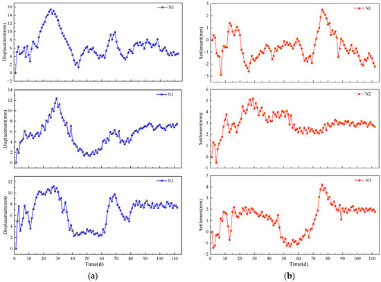
Figure 4.
Deformation monitoring results of the first section of the portal slope: (a) horizontal displacement value, (b) vertical displacement value.

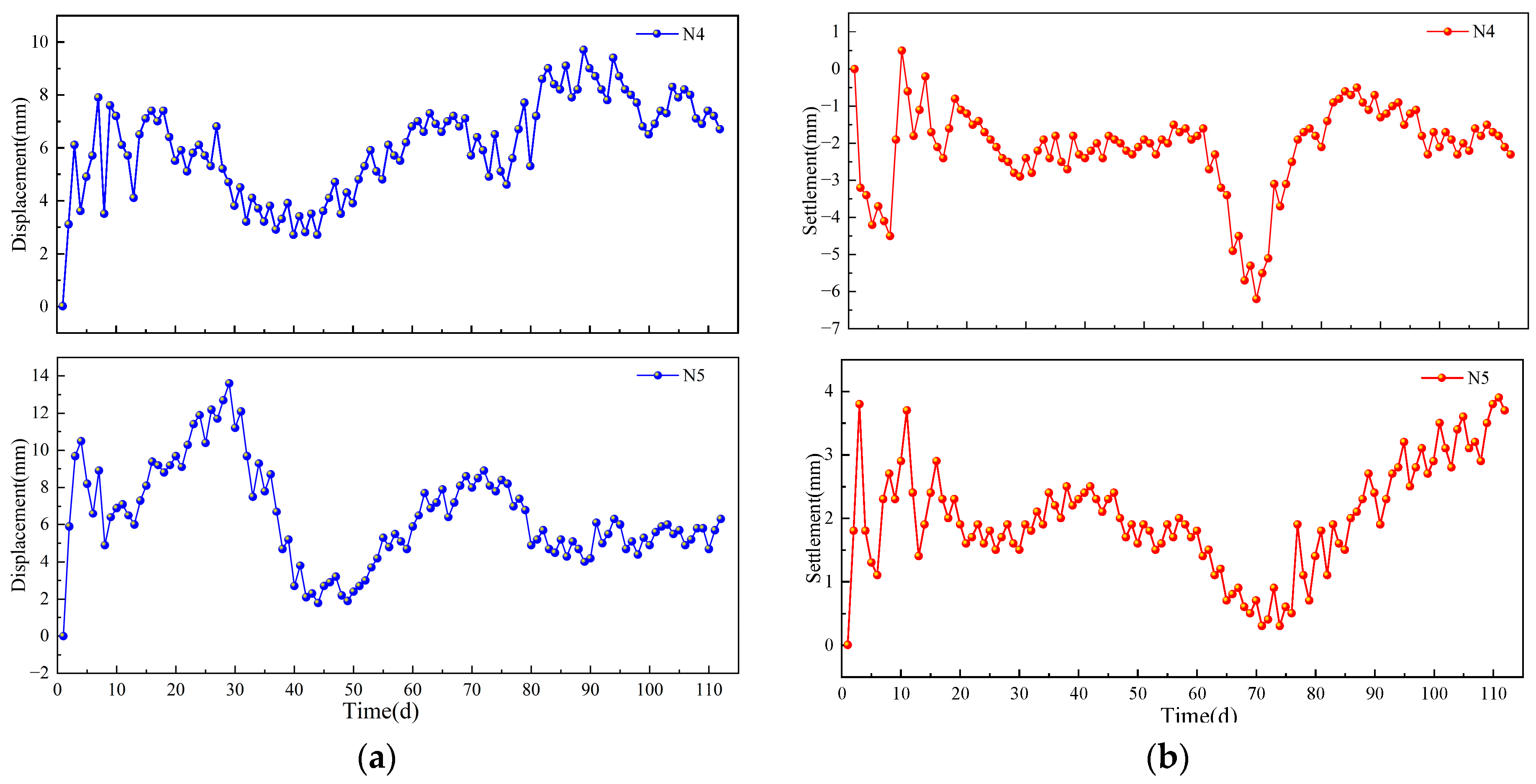
Figure 5.
Deformation monitoring results of the second section of the portal slope: (a) horizontal displacement value, (b) vertical displacement value.

Figure 6.
Deformation monitoring results of the third section of the portal slope: (a) horizontal displacement value, (b) vertical displacement value.
As can be seen from Figure 4, the trends of horizontal displacement at the three monitoring points in the first section of the tunnel portal slope are basically the same. The horizontal displacements peaked at about the 25th day, which were 15.4 mm, 12.4 mm, and 11.2 mm, respectively, and the horizontal displacements at the monitoring points stabilized after the 85th day. The horizontal displacements after deformation stabilization were about 4.5 mm, 7.0 mm, and 7.5 mm. The vertical displacements at monitoring points N1 and N3 of the tunnel portal slope had similar trends. The vertical displacement at monitoring point N1 was characterized by settlement. However, the displacement at monitoring point N3 shows upward bulging. The vertical displacements peaked at about day 75 at 2.5 mm and 4.2 mm, respectively. The settlement value of monitoring point N3 stabilized after 90 days, and the stabilized vertical displacement was about 2.0 mm. The settlement value of monitoring point N2 peaked at about 25 days at 5.1 mm. The settlement value of monitoring point N2 stabilized after 60 days, and the stabilized vertical displacement was about 3.0 mm. The vertical displacements of monitoring points N1 and N3 are similar in trend.
As can be seen from Figure 5, the horizontal displacement at monitoring point N4 in the second section of the tunnel portal slope peaked at 9.4 mm on the 90th day, while the horizontal displacement at monitoring point N5 peaked at 13.6 mm on the 25th day, and the horizontal displacement stabilized after the 80th day. The horizontal displacement after stabilization is about 5.5 mm. The vertical displacement value of the N4 monitoring point on the slope of the tunnel entrance reached its peak on the 70th day, which was −6.2 mm. The vertical displacement value tends to stabilize after the 95th day, and the settlement after stabilization is about −2.0 mm. The vertical displacement value of the N5 monitoring point has not yet stabilized after the 100th point, with a vertical displacement value greater than 4.0 mm. However, the vertical displacement of the N5 monitoring point shows an upward uplift.
As can be seen from Figure 6, the trend of horizontal displacement at the monitoring points of the third section of the tunnel portal slope is basically the same. The horizontal displacements peaked at about the 28th day, at 14.9 mm and 12.3 mm, respectively, and the horizontal displacements at N7 tended to stabilize after the 90th day. The horizontal displacement after stabilization is about 6.3 mm. The vertical displacement values of the three sections of the tunnel portal side slope monitoring points show multiple peaks of about −3 mm. The vertical displacement value of the N7 monitoring point still does not stabilize after the 100th day, and the performance of the vertical displacement changes from settlement to upward bulging.
From the above analysis, it can be seen that during the monitoring period, the maximum value of horizontal displacement of the slope at the entrance is 15.4 mm, and the maximum value of vertical settlement is −6.2 mm, and after the deformation and stabilization of the slope at the entrance, the horizontal displacement is about 6–8 mm, and the value of vertical settlement is not more than −2 mm. Therefore, the horizontal displacement and vertical settlement of the slope at the entrance are small, and the stability of the slope at the entrance of the tunnel is relatively high.
3.2. MultiFractal Characteristics of Deformation of Elevation Slope at Tunnel Portals
3.2.1. Horizontal Displacement Multifractal Characterization
The sliding time window optimization MF-DFA is used to perform multifractal analysis on the deformation monitoring sequences of each monitoring point of the side slope of the tunnel portal, respectively. The generalized Hurst exponent and Renyi exponent are computed for the horizontal displacement sequences at each monitoring point. The variation of the indices corresponding to the sequence of monitoring points is shown in Figure 7. Further, the multifractal spectrum of the horizontal displacement sequence is shown in Figure 8.

Figure 7.
Variation of each index of the horizontal displacement series: (a) generalized Hurst index, (b) scaling function τ(q).
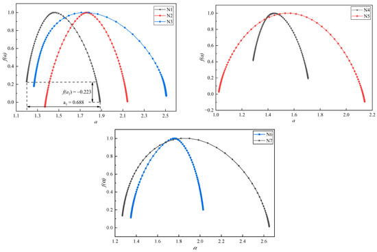
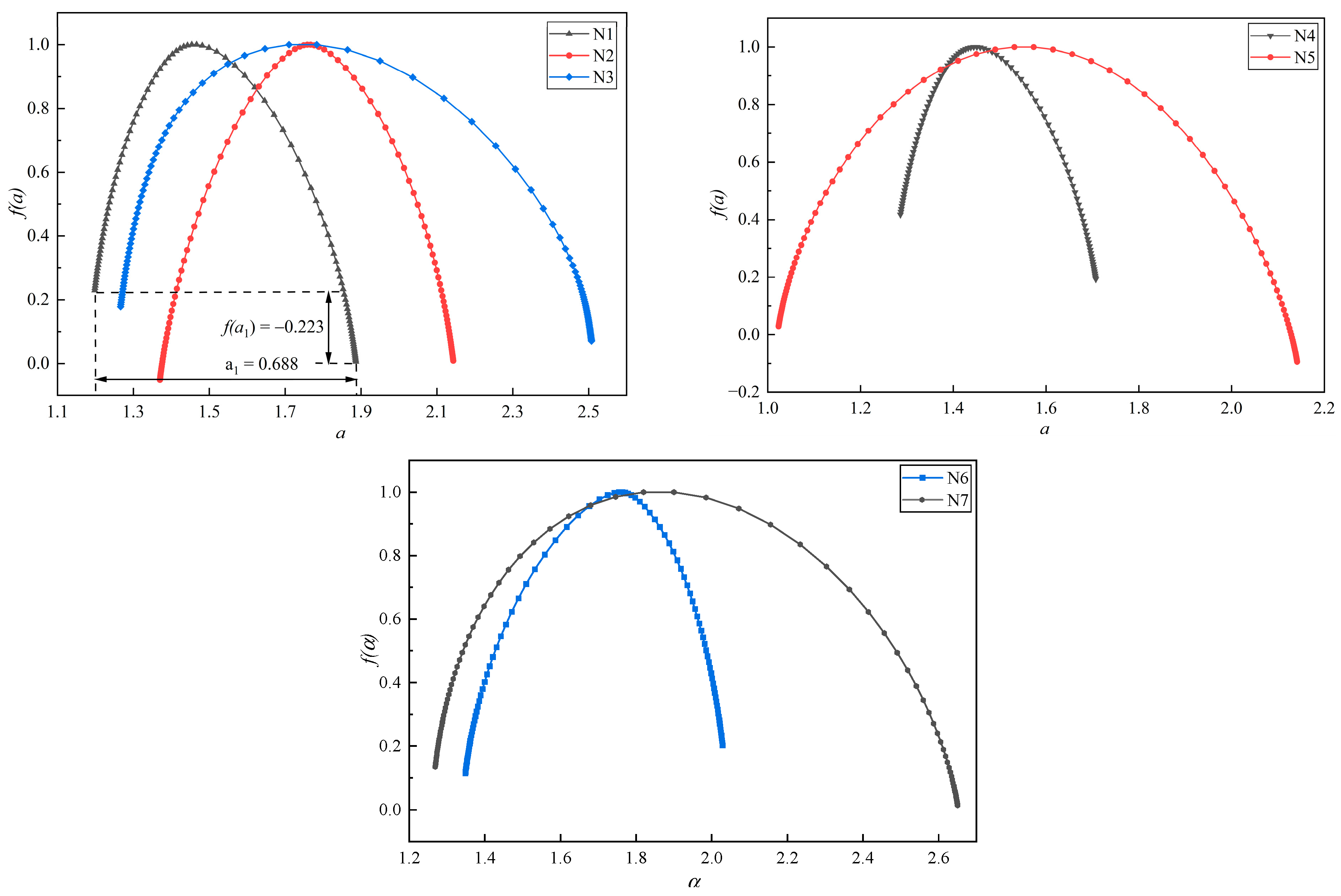
Figure 8.
Multifractal spectrum of the horizontal displacement sequence.
As can be seen from Figure 7, when q varies between [−10,10], the generalized Hurst indices of the horizontal displacement sequences of different monitoring sections of the tunnel portal slope sides are all nonlinearly decreasing with q. The generalized Hurst indices of the horizontal displacement sequences of different monitoring sections of the elevation slope of the tunnel portal are all nonlinearly decreasing with q. This indicates that the horizontal displacement sequences at each monitoring point are characterized by multifractal. Under different fluctuation orders q, the generalized Hurst exponent curves of the horizontal displacement series at N1, N2, N4, and N6 are concentrated in the lower fluctuation of N3, N5, and N7, which show a weaker multifractal characteristic. However, the values of the horizontal displacement series at each monitoring point are significantly larger than 0.5. values are significantly larger than 0.5, indicating that all the monitoring point sequences have better memory and long-range correlation from the whole to the local components. In addition, from Figure 7, it can be seen that the scale function of the horizontal displacement series at each monitoring point is in good agreement. The middle part of the scale function curve is upconvex, satisfies , as well as the overall nonlinear relationship. It indicates that the horizontal displacement sequence of each monitoring point has multifractal characteristics.
As can be seen in Figure 8, for the multifractal spectra of the horizontal displacement sequences of the monitoring points at different monitoring sections, the images of the multifractal spectra show a typical single-peak convex distribution, which resembles a quadratic function curve. The local scales of the multifractals of the horizontal displacement series are not constant, indicating the diversity of local changes at different moments. The singular intensities of most of the horizontal displacement sequences are distributed on both sides of the image, reflecting the diversity of local variations at different moments. are distributed on both sides of the image, reflecting the uneven distribution of the fractal structure of the monitoring point sequences. This further illustrates the multifractal nature of the horizontal displacement sequence. The multifractal spectral curves of the horizontal displacement sequences are basically symmetrical, and the overall development state is stable.
In Figure 8, represents the multifractal spectral width, which signifies the multifractal strength and complexity of the fluctuations at the monitoring point. A larger indicates stronger multifractal strength and more intense, complex fluctuations in the sequence. Meanwhile, denotes the proportion of large and small fluctuations in the sequence. A higher signifies a greater proportion of small and medium fluctuations in the sequence. The calculations for and are as follows:
Calculate the multifractal characteristic statistics of the horizontal displacement series of the monitoring points of different monitoring sections; the calculation results are shown in Table 1.

Table 1.
Multifractal characteristic statistics for horizontal displacement.
As can be seen from Table 1, comparing the width of the multifractal spectrum of the horizontal displacement sequence at each monitoring point . For Section 1, the multifractal spectral widths of the horizontal displacement sequences at monitoring points N1 and N2 are smaller than those at monitoring point N3. is smaller than that of N3. It means that the multifractal intensity of the horizontal displacement sequence at N3 is larger, and the horizontal displacement fluctuation is more complicated. Similarly, for Sections 2 and 3, the multifractal intensity of the horizontal displacement series at points N5 and N7 is larger, and the displacement fluctuations are more complicated. Comparison of the proportion of large and small fluctuations in the horizontal displacement series at each monitoring point. The proportion of large and small fluctuations in the horizontal displacement sequence of each monitoring point is compared. For Section 1, the horizontal displacement sequence of N2 is slightly larger than that of N1 and N3. is slightly larger than that of N1 and N3. This indicates that the proportion of small fluctuations in the horizontal displacement sequence at N2 is larger. Similarly, for Sections 2 and 3, the proportion of small fluctuations in the horizontal displacement sequences of monitoring points N5 and N6 is larger than that of monitoring points N1 and N3.
It can be seen that the results of the multifractal eigenvalues of the horizontal displacement sequences of different monitoring sections at the tunnel portal are more in line with the actual monitoring results, and the multifractal intensity of the horizontal displacement sequences at monitoring points N3, N5, and N7 is more intense, and the fluctuation of the displacement sequences at the monitoring points is slightly more complicated. When evaluating the stability of the tunnel portal slope, more attention should be paid to the horizontal displacement changes at monitoring points N3, N5, and N7.
3.2.2. Vertical Displacement Multifractal Characterization
The multifractal analysis is performed on the vertical displacement sequences of each monitoring point of the upward slope of the tunnel portal respectively. The generalized Hurst index, Renyi index, and multifractal spectrum of the vertical displacement sequence at each monitoring point are obtained, and the index changes of the corresponding monitoring point sequence are shown in Figure 9 and Figure 10.

Figure 9.
Variation of each index of the vertical displacement sequence: (a) generalized Hurst index, (b) scaling function τ(q).

Figure 10.
Multifractal spectrum of vertical displacement sequence.
As can be seen from Figure 9, when q varies between [−10,10], the generalized Hurst indices of the vertical displacement sequences of different monitoring sections of the tunnel portal slope are all nonlinearly decreasing with q. The generalized Hurst indices of the vertical displacement sequences of different monitoring sections of the tunnel portal slope are all nonlinearly decreasing with q. This indicates that the vertical displacement sequences at each monitoring point are characterized by multifractal. At different fluctuation orders q, the values of the vertical displacement series at each monitoring point are significantly larger than 0.5, indicating that all the sequences have good memory and long-range correlation from the whole to the local components. In addition, from Figure. 9, it can be seen that the scale function of the vertical displacement series at each monitoring point is in good agreement. The middle part of the scalar function curve is upconvex and satisfies The scale function curve has an upward convex shape in the center, which indicates that the vertical displacement sequence of each monitoring point has multifractal characteristics.
In Figure 10, the multifractal spectra of the vertical displacement sequences at various monitoring points across different sections exhibit a distinctive single-peak convex distribution, resembling a quadratic function curve. The local scales of these multifractals display variability, highlighting the diverse local changes occurring at different instances. The singular intensities of the vertical displacement sequences are dispersed on both sides of the image, showcasing the heterogeneous local variations over time. The distribution of α values on either side of the image further underscores the uneven fractal structure distribution within the monitoring point sequence, emphasizing its multifractal nature. Notably, the multifractal spectral curves of the vertical displacement sequences exhibit a symmetrical pattern, indicating a stable overall development state.
Calculate the multifractal characteristic statistics of the vertical displacement sequences of monitoring points in different monitoring sections; the calculation results are shown in Table 2.
Table 2.
Vertical displacement multifractal characterization statistics.
As can be seen from Table 2, we compare the widths of the multifractal spectra of the vertical displacement series at each monitoring point . For Section 1, the multifractal spectral widths of the vertical displacement sequences at monitoring points N1 and N2 are smaller than those at monitoring point N3. is smaller than that of N3. This means that the vertical displacement sequence at N3 has a larger intensity of multifractals, and the vertical displacement fluctuation is more complicated. Similarly, for Sections 2 and 3, the multifractal strengths of the vertical displacement series at N4 and N6 are larger, and the displacement fluctuations are more complicated. Comparing the proportion of large and small fluctuations in the vertical displacement series at each monitoring point, the proportion of large and small fluctuations in the vertical displacement series at N4 and N6 is larger. The proportion of large and small fluctuations in the vertical displacement sequences at each monitoring point is compared. For Section 1, the vertical displacement sequence at monitoring point N2 is slightly larger than that at monitoring points N1 and N3. This indicates that the proportion of small fluctuations in the vertical displacement sequence at N2 is larger. Similarly, for Sections 2 and 3, the proportion of small fluctuations in the vertical displacement sequences of monitoring points N5 and N7 is larger.
It can be seen that the results of the multifractal eigenvalues of the vertical displacement sequences of different monitoring sections at the tunnel portal side slope are more in line with the actual monitoring results, and the multifractal strengths of the vertical displacement sequences at monitoring points N3, N4, and N6 are more intense, and the fluctuations of the displacement sequences of the monitoring points are slightly more complicated. More attention should be paid to the vertical displacement changes at monitoring points N3, N4, and N6 when evaluating the stability of the tunnel portal slope.
3.3. PSO-LSTM Prediction of Slope Deformation at Tunnel Portal Sides
The results of the previous study show that the results of the multifractal eigenvalues of the displacement sequences of the different monitoring sections of the tunnel portal slope are more in line with the actual monitoring results. Among them, the horizontal displacements at N3, N5, and N7 are more intense, and the vertical displacements at N3, N4, and N6 are more intense. Therefore, the PSO-LSTM method is used to predict the horizontal displacements at N3, N5, and N7 and the vertical displacements at N3, N4, and N6 when evaluating the stability of the tunnel portal slope.
3.3.1. Horizontal Displacement Prediction Results
The hyperparameters obtained after PSO optimization are used to input the LSTM model. Model training is performed on the input data. Based on several iterations and training, the accuracy of the model prediction was made to reach a reasonable range. The daily data of monitoring data from different monitoring sections of the tunnel portal slope were selected for prediction, totaling about 100 sets of data. Furthermore, 70% of the data is used as the training set and the remaining 30% of the data is the test set. The PSO-LSTM model was trained and tested, and the predicted horizontal displacements of the N3, N5, and N7 monitoring points of the tunnel portal slope are shown in Figure 11.
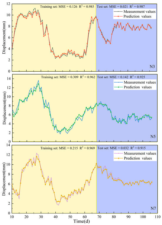
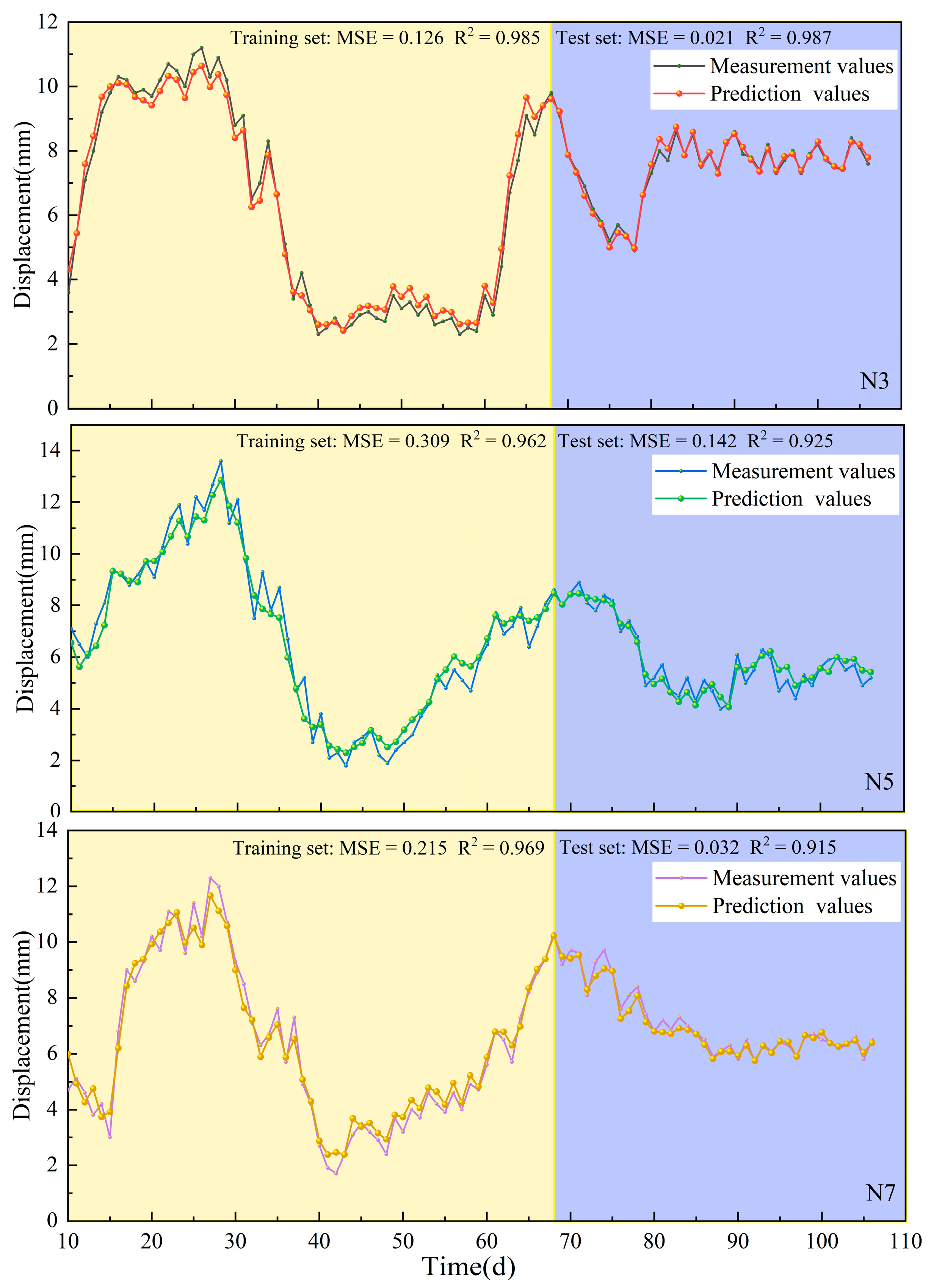
Figure 11.
Predicted horizontal displacement of the tunnel portal slope.
As can be seen from Figure 11, the PSO-LSTM model predicts the horizontal displacements of the tunnel portal slope at monitoring points N3, N5, and N7, which are closer to the actual monitoring results. The maximum MSE value of the horizontal displacement training set fitting results for each measurement point is 0.309, and the R2 is higher than 96%. The maximum MSE value of the prediction results of the test set is 0.142, and the R2 is higher than 91%. From the prediction curves, it can be seen that the predicted horizontal displacements of measuring points N3 and N7 after the 85th day almost coincide with the actual monitoring results. It can be seen that the PSO-LSTM model is more effective in predicting the horizontal displacement in the middle and late stages of the monitoring sequence.
To further evaluate the error between the PSO-LSTM model’s prediction of horizontal displacement sequences at monitoring points N3, N5, and N7 and the measured values, the results of the PSO-LSTM model’s horizontal displacement prediction error calculations are shown in Figure 12.

Figure 12.
Calculation results of horizontal displacement prediction error.
As can be seen from Figure 12, by comparing the sample error calculation results of the PSO-LSTM model for the prediction of the horizontal displacement sequences of the N3, N5, and N7 monitoring points, it is found that the maximum value of the horizontal displacement prediction error of the N3 monitoring point is 0.81 mm. It is found that the maximum value of the horizontal displacement prediction error of the N3 monitoring point is 0.81 mm, and about 90% of the sample prediction errors can be controlled within ±0.5 mm, the maximum value of the horizontal displacement prediction error of the N5 monitoring point is −1.6 mm, about 90% of the sample prediction errors can be controlled within ±0.8 mm, the maximum value of the horizontal displacement prediction error of the N7 monitoring point is 1.29 mm, and about 90% of the sample prediction errors can be controlled within ±0.6 mm can be controlled within ±0.6 mm. It can be seen from the figure that the maximum prediction error of the model test set is significantly smaller than the training set prediction error. It shows that the PSO-LSTM model can predict the horizontal displacement sequences of N3, N5, and N7 with small sample errors. This indicates that the PSO-LSTM prediction model has better performance.
3.3.2. Vertical Displacement Prediction Results
The PSO-LSTM model was trained and tested to predict the vertical displacements at the N3, N4, and N6 monitoring points on the portal slope of the tunnel portal. The corresponding prediction results are shown in Figure 13.

Figure 13.
Vertical displacement prediction results of tunnel portal slope.
As can be seen from Figure 13, the PSO-LSTM model predicts the vertical displacements of the tunnel portal slope at monitoring points N3, N4, and N6, which are closer to the actual monitoring results. The maximum MSE value of the vertical displacement training set fitting results for each measurement point is 0.078, and the R2 is higher than 93%. The maximum MSE value of the prediction results of the test set is 0.069, and the R2 is higher than 91%. From the prediction curves, it can be seen that the predicted vertical displacements of monitoring points N3 and N6 after the 75th day almost coincide with the actual monitoring results. It can be seen that the PSO-LSTM model is more effective in predicting the vertical displacement monitoring sequence in the middle and late stages.
To further evaluate the error between the PSO-LSTM model’s prediction of vertical displacement sequences at monitoring points N3, N4, and N6 and the measured values, the results of the PSO-LSTM model’s vertical displacement prediction error calculations are shown in Figure 14.

Figure 14.
Calculation results of vertical displacement prediction error.
As can be seen in Figure 14, by comparing the sample error calculation results of the PSO-LSTM model for the prediction of vertical displacement sequences at the N3, N4, and N6 monitoring points, it is found that the maximum value of the prediction error of vertical displacement at N3 is 0.58 mm, and about 90% of the sample prediction errors can be controlled within ±0.2 mm, the maximum value of the prediction error of vertical displacement at N4 is 0.85 mm, and about 90% of the sample prediction errors can be controlled within ±0.35 mm. The maximum value of the prediction error of vertical displacement at N6 is −0.77 mm and about 90% of the sample prediction errors can be controlled within ±0.30 mm. The maximum prediction error of vertical displacement at N6 is −0.77 mm, and the prediction error of about 90% of the samples can be controlled within ±0.30 mm. From the figure, it can be seen that the maximum prediction error of the model test set is slightly smaller than the training set error. It shows that the PSO-LSTM model predicts the vertical displacement sequences of the N3, N4, and N6 monitoring points with small sample errors. It shows that the PSO-LSTM model has good performance and can meet the requirements of vertical displacement prediction for the tunnel portal slope.
4. Discussion
Tunnel construction is often challenging due to the presence of difficult geological conditions such as high slopes, bias pressure, and shallow burial. These conditions can lead to engineering accidents like collapse, slope instability, and landslides during the tunnel portal construction. As a result, ensuring the stability of the surrounding rock and side slopes at the tunnel portal has become a crucial focus of research in tunnel engineering. In the theoretical study of the stability of the surrounding rock at the tunnel portal, numerical simulation is commonly used to analyze the tunnel and its entrance slope [19,22,24]. Some scholars have also carried out large-scale shaking table tests to determine the macro damage of tunnel lining and entrance slopes. Additionally, monitoring slope displacement in the tunnel portal section is deemed essential for field application. Various excavation methods for shallow tunnels have been adopted to control deformation and stabilize slopes at the entrance. However, the complexity of tunnel portal slope engineering as a nonlinear dynamic system means that stability and deformation are influenced by numerous uncertain factors. Theoretical methods like numerical simulation may not fully guarantee stability during tunnel excavation, especially in unfavorable geological conditions. Continuous monitoring of entrance side slope elevation is necessary to analyze deformation trends, predict displacement development, and prevent tunnel disasters.
To address challenges in constructing a weak, water-rich, and shallow buried tunnel portal next to an important structure, this study focuses on designing a monitoring and measurement scheme to analyze tunnel portal side slope deformation. Monitoring results indicate high stability after stabilization, with minimal horizontal and vertical displacement. By using the MF-DFA method, the study analyzes multifractal characteristics of monitoring sequences at each measurement point of the tunnel portal slope. Results show good consistency with actual monitoring data, revealing higher multifractal intensity in horizontal and vertical displacement sequences at certain measurement points. Furthermore, the PSO-LSTM model is utilized to predict displacement developments at measurement points on the tunnel portal slope. Prediction accuracy is notably high, indicating the model’s effectiveness in forecasting displacement sequences.
In conclusion, tunnel portal sections face challenges in unfavorable geological environments, making it crucial to mitigate engineering risks and ensure stability. Analyzing and predicting slope monitoring data can inform dynamic design, optimize tunnel excavation and support programs, and enhance the safety and stability of adjacent structures like high-voltage towers.
5. Conclusions
Analyzing and predicting the deformation pattern of the portal slope during tunnel portal construction can provide technical support and theoretical guidance for the early warning of tunnel portal section construction safety. Therefore, this paper takes the construction of a soft, water-rich, and shallow buried tunnel portal section near a high-voltage power tower in Malaysia as the background. Combined with on-site monitoring, multifractal analysis, and deep learning methods, it carries out an in-depth study of the multifractal characteristics and displacement prediction of the deformation of the tunnel portal slope. The main research conclusions are as follows.
- Combined with the deformation characteristics of the tunnel portal slope, design a suitable monitoring and measuring program to analyze the deformation pattern of the tunnel portal slope. After the deformation of the tunnel portal slope is stabilized, the horizontal displacement is about 6–8 mm, the vertical settlement value is not more than 2 mm, and the stability of the tunnel portal slope is high.
- Based on the MF-DFA method, analyze the multifractal characteristics of the deformation monitoring sequences at each monitoring point of the tunnel portal slope. The MF eigenvalues of the displacement sequences at different monitoring sections of the tunnel portal slope are more in line with the actual monitoring results. For the horizontal displacement sequences, the multifractal strengths of monitoring points N3, N5, and N7 are larger. For the vertical displacement sequence, the multifractal intensities of monitoring points N3, N4, and N6 are larger.
- The PSO-LSTM prediction model was utilized to predict the deformation development of the side slope of the tunnel portal. The maximum MSE value of the horizontal displacement test set prediction result is 0.142, and R2 is higher than 91%. The maximum MSE value of the vertical displacement test set prediction result is 0.069, and R2 is higher than 91%. The PSO-LSTM model has a small error in predicting the displacement sequence of each monitoring point, and the performance of the prediction model can meet the requirements for predicting the displacement of the portal slope of the tunnel portal.
The tunnel portal section under study has a single nature of surrounding rock, and the values of side and elevation slope deformation are generally small. In future studies, multifractal characterization can be carried out to analyze the slope displacement sequences of tunnels with different surrounding rock properties. In addition, more factors affecting the slope deformation can be considered to further improve the prediction accuracy of the PSO-LSTM model.
Author Contributions
Methodology, X.Z. and Y.H.; software, W.Z.; validation, X.Z. and Y.H.; formal analysis, W.Z. and D.L.; data curation, X.Z. and W.Z.; writing—original draft preparation, W.Z.; writing—review and editing, X.Z. and D.L.; project administration, Y.H. and D.L.; funding acquisi-tion, X.Z. and Y.H. All authors have read and agreed to the published version of the manuscript.
Funding
This research received no external funding.
Data Availability Statement
The data that support the findings of this study are available upon request from the authors.
Acknowledgments
The authors would like to thank Road & Bridge International Co., Ltd. for their assistance with conducting the field experiments.
Conflicts of Interest
Authors Xiannian Zhou and Yurui He were employed by the company Road & Bridge International Co., Ltd. The remaining authors declare that the research was conducted in the absence of any commercial or financial relationships that could be construed as a potential conflict of interest.
References
- Gong, C.; Ding, W.; Mosalam, K.M.; Gunay, S.; Soga, K. Comparison of the structural behavior of reinforced concrete and steel fiber reinforced concrete tunnel segmental joints. Tunn. Undergr. Space Technol. 2017, 68, 38–57. [Google Scholar] [CrossRef]
- Lei, M.; Liu, L.; Shi, C.; Tan, Y.; Lin, Y.; Wang, W. A novel tunnel-lining crack recognition system based on digital image technology. Tunn. Undergr. Space Technol. 2021, 108, 103724. [Google Scholar] [CrossRef]
- Zhou, Z.; Zhang, J.; Gong, C. Automatic detection method of tunnel lining multi-defects via an enhanced You Only Look Once network. Comput.-Aided Civ. Infrastruct. Eng. 2022, 37, 762–780. [Google Scholar] [CrossRef]
- Bandini, A.; Berry, P.; Boldini, D. Tunnelling-induced landslides: The Val di Sambro tunnel case study. Eng. Geol. 2015, 196, 71–87. [Google Scholar] [CrossRef]
- Zhao, C.; Lei, M.; Shi, C.; Cao, H.; Yang, W.; Deng, E. Function mechanism and analytical method of a double layer pre-support system for tunnel underneath passing a large-scale underground pipe gallery in water-rich sandy strata: A case study. Tunn. Undergr. Space Technol. 2021, 115, 104041. [Google Scholar] [CrossRef]
- Jia, C.; Zhang, Q.; Lei, M.; Zheng, Y.; Huang, J.; Wang, L. Anisotropic properties of shale and its impact on underground structures: An experimental and numerical simulation. Bull. Eng. Geol. Environ. 2021, 80, 7731–7745. [Google Scholar] [CrossRef]
- Huang, L.; Ma, J.; Lei, M.; Liu, L.; Lin, Y.; Zhang, Z. Soil-water inrush induced shield tunnel lining damage and its stabilization: A case study. Tunn. Undergr. Space Technol. 2020, 97, 103290. [Google Scholar] [CrossRef]
- Lei, M.; Lin, D.; Huang, Q.; Shi, C.; Huang, L. Research on the construction risk control technology of shield tunnel underneath an operational railway in sand pebble formation: A case study. Eur. J. Environ. Civ. Eng. 2020, 24, 1558–1572. [Google Scholar] [CrossRef]
- Zhang, Y.; Yang, J.; Yang, F. Field investigation and numerical analysis of landslide induced by tunneling. Eng. Fail. Anal. 2015, 47, 25–33. [Google Scholar] [CrossRef]
- Zhou, Z.; Ding, H.; Miao, L.; Gong, C. Predictive model for the surface settlement caused by the excavation of twin tunnels. Tunn. Undergr. Space Technol. 2021, 114, 104014. [Google Scholar] [CrossRef]
- Aygar, E.B.; Gokceoglu, C. Effects of Portal Failure on Tunnel Support Systems in a Highway Tunnel. Geotech. Geol. Eng. 2021, 39, 5707–5726. [Google Scholar] [CrossRef]
- Ayoublou, F.F.; Taromi, M.; Eftekhari, A. Tunnel portal instability in landslide area and remedial solution: A case study. Acta Polytech. 2019, 59, 435–447. [Google Scholar] [CrossRef]
- Kaya, A.; Karaman, K.; Bulut, F. Geotechnical investigations and remediation design for failure of tunnel portal section: A case study in northern Turkey. J. Mt. Sci. 2017, 14, 1140–1160. [Google Scholar] [CrossRef]
- Lei, M.; Li, J.; Zhao, C.; Shi, C.; Yang, W.; Deng, E. Pseudo-dynamic analysis of three-dimensional active earth pressures in cohesive backfills with cracks. Soil Dyn. Earthq. Eng. 2021, 150, 106917. [Google Scholar] [CrossRef]
- Wang, Q.; Geng, P.; Li, P.; Chen, J.; He, C. Dynamic damage identification of tunnel portal and verification via shaking table test. Tunn. Undergr. Space Technol. 2023, 132, 104923. [Google Scholar] [CrossRef]
- Wang, Q.; Geng, P.; Chen, J.; He, C. Dynamic discrimination method of seismic damage in tunnel portal based on improved wavelet packet transform coupled with Hilbert-Huang transform. Mech. Syst. Signal Process. 2023, 188, 110023. [Google Scholar] [CrossRef]
- Genis, M. Assessment of the dynamic stability of the portals of the Dorukhan tunnel using numerical analysis. Int. J. Rock Mech. Min. Sci. 2010, 47, 1231–1241. [Google Scholar] [CrossRef]
- Tuncay, E. Assessments on slope instabilities triggered by engineering excavations near a small settlement (Turkey). J. Mt. Sci. 2018, 15, 114–129. [Google Scholar] [CrossRef]
- Wang, X.; Chen, J.; Zhang, Y.; Xiao, M. Seismic responses and damage mechanisms of the structure in the portal section of a hydraulic tunnel in rock. Soil Dyn. Earthq. Eng. 2019, 123, 205–216. [Google Scholar] [CrossRef]
- Jia, J. Application of PS-INSAR Technique on Health Diagnosis of the Deformable Body on Front Slope beside Mountain Tunnel Portal. Math. Probl. Eng. 2020, 2020, 8823382. [Google Scholar] [CrossRef]
- Feng, H.; Jiang, G.; He, Z.; Guo, Y.; Hu, J.; Li, J.; Yuan, S. Dynamic response characteristics of tunnel portal slope reinforced by prestressed anchor sheet-pile wall. Rock Soil Mech. 2023, 44S, 50–62. [Google Scholar]
- Zhang, Q.; Wang, J.; Zhang, H. Attribute recognition model and its application of risk assessment for slope stability at tunnel portal. J. Vibroeng. 2017, 19, 2726–2738. [Google Scholar] [CrossRef]
- Li, X.; Li, X.; Yang, C. A comparison study of face stability between the entering and exiting a shallow-buried tunnel with a front slope. Front. Earth Sci. 2022, 10, 987294. [Google Scholar] [CrossRef]
- Li, C.; Zheng, H.; Hu, Z.; Liu, X.; Huang, Z. Analysis of Loose Surrounding Rock Deformation and Slope Stability at Shallow Double-Track Tunnel Portal: A Case Study. Appl. Sci. 2023, 13, 50248. [Google Scholar] [CrossRef]
- Aygar, E.B.; Gokceoglu, C. Problems Encountered during a Railway Tunnel Excavation in Squeezing and Swelling Materials and Possible Engineering Measures: A Case Study from Turkey. Sustainability 2020, 12, 11663. [Google Scholar] [CrossRef]
- Taromi, M.; Eftekhari, A.; Hamidi, J.K.; Aalianvari, A. A discrepancy between observed and predicted NATM tunnel behaviors and updating: A case study of the Sabzkuh tunnel. Bull. Eng. Geol. Environ. 2017, 76, 713–729. [Google Scholar] [CrossRef]
- Zhu, B.; Lei, M.; Gong, C.; Zhao, C.; Zhang, Y.; Huang, J.; Jia, C.; Shi, C. Tunnelling-induced landslides: Trigging mechanism, field observations and mitigation measures. Eng. Fail. Anal. 2022, 138, 106387. [Google Scholar] [CrossRef]
- Xi, N.; Yang, Q.; Sun, Y.; Mei, G. Machine Learning Approaches for Slope Deformation Prediction Based on Monitored Time-Series Displacement Data: A Comparative Investigation. Appl. Sci. 2023, 13, 46778. [Google Scholar] [CrossRef]
- Intrieri, E.; Gigli, G.; Mugnai, F.; Fanti, R.; Casagli, N. Design and implementation of a landslide early warning system. Eng. Geol. 2012, 147, 124–136. [Google Scholar] [CrossRef]
- Dai, F.C.; Lee, C.F.; Ngai, Y.Y. Landslide risk assessment and management: An overview. Eng. Geol. 2002, 64, 65–87. [Google Scholar] [CrossRef]
- Lopes, R.; Betrouni, N. Fractal and multifractal analysis: A review. Med. Image Anal. 2009, 13, 634–649. [Google Scholar] [CrossRef]
- Liu, J.; Li, Q.; Wang, X.; Wang, Z.; Lu, S.; Sa, Z.; Wang, H. Dynamic multifractal characteristics of acoustic emission about composite coal-rock samples with different strength rock. Chaos Soliton Fract. 2022, 164, 112725. [Google Scholar] [CrossRef]
- Ehlen, J. Fractal analysis of joint patterns in granite. Int. J. Rock Mech. Min. Sci. 2000, 37, 909–922. [Google Scholar] [CrossRef]
- Li, W.; Zhao, H.; Wu, H.; Wang, L.; Sun, W.; Ling, X. A novel approach of two-dimensional representation of rock fracture network characterization and connectivity analysis. J. Petrol. Sci. Eng. 2020, 184, 106507. [Google Scholar] [CrossRef]
- Zhang, W.; Liu, D.; Tang, Y.; Qiu, W.; Zhang, R. Multifractal Characteristics of Smooth Blasting Overbreak in Extra-Long Hard Rock Tunnel. Fractal Fract. 2023, 7, 84212. [Google Scholar] [CrossRef]
- Liu, D.; Zhang, W.; Jian, Y.; Tang, Y.; Cao, K. Damage precursors of sulfate erosion concrete based on acoustic emission multifractal characteristics and b-value. Constr. Build. Mater. 2024, 419, 135380. [Google Scholar] [CrossRef]
- Wasowski, J.; Bovenga, F. Investigating landslides and unstable slopes with satellite Multi Temporal Interferometry: Current issues and future perspectives. Eng. Geol. 2014, 174, 103–138. [Google Scholar] [CrossRef]
- Gariano, S.L.; Guzzetti, F. Landslides in a changing climate. Earth-Sci. Rev. 2016, 162, 227–252. [Google Scholar] [CrossRef]
- Li, Z.; Cheng, P.; Zheng, J. Prediction of time to slope failure based on a new model. Bull. Eng. Geol. Environ. 2021, 80, 5279–5291. [Google Scholar] [CrossRef]
- Feng, X.T.; Zhao, H.B.; Li, S.J. Modeling non-linear displacement time series of geo-materials using evolutionary support vector machines. Int. J. Rock Mech. Min. Sci. 2004, 41, 1087–1107. [Google Scholar] [CrossRef]
- Huang, Y.; Zhao, L. Review on landslide susceptibility mapping using support vector machines. Catena 2018, 165, 520–529. [Google Scholar] [CrossRef]
- Ma, Z.; Mei, G.; Prezioso, E.; Zhang, Z.; Xu, N. A deep learning approach using graph convolutional networks for slope deformation prediction based on time-series displacement data. Neural Comput. Appl. 2021, 33, 14441–14457. [Google Scholar] [CrossRef]
- Ma, Z.; Mei, G.; Piccialli, F. Machine learning for landslides prevention: A survey. Neural Comput. Appl. 2021, 33, 10881–10907. [Google Scholar] [CrossRef]
- Xiao, L.; Zhang, Y.; Peng, G. Landslide Susceptibility Assessment Using Integrated Deep Learning Algorithm along the China-Nepal Highway. Sensors 2018, 18, 443612. [Google Scholar] [CrossRef]
- Lian, C.; Zeng, Z.; Yao, W.; Tang, H. Multiple neural networks switched prediction for landslide displacement. Eng. Geol. 2015, 186, 91–99. [Google Scholar] [CrossRef]
- Pei, H.; Meng, F.; Zhu, H. Landslide displacement prediction based on a novel hybrid model and convolutional neural network considering time-varying factors. Bull. Eng. Geol. Environ. 2021, 80, 7403–7422. [Google Scholar] [CrossRef]
- Wang, H.; Zhang, L.; Luo, H.; He, J.; Cheung, R.W.M. AI-powered landslide susceptibility assessment in Hong Kong. Eng. Geol. 2021, 288, 106103. [Google Scholar] [CrossRef]
- Yang, B.; Yin, K.; Lacasse, S.; Liu, Z. Time series analysis and long short-term memory neural network to predict landslide displacement. Landslides 2019, 16, 677–694. [Google Scholar] [CrossRef]
- Liu, Z.; Gilbert, G.; Cepeda, J.M.; Lysdahl, A.O.K.; Piciullo, L.; Hefre, H.; Lacasse, S. Modelling of shallow landslides with machine learning algorithms. Geosci. Front. 2021, 12, 385–393. [Google Scholar] [CrossRef]
- Yan, L.; Chen, C.; Hang, T.; Hu, Y. A stream prediction model based on attention-LSTM. Earth Sci. Inform. 2021, 14, 723–733. [Google Scholar] [CrossRef]
- Li, C.; Li, J.; Shi, Z.; Li, L.; Li, M.; Jin, D.; Dong, G. Prediction of Surface Settlement Induced by Large-Diameter Shield Tunneling Based on Machine-Learning Algorithms. Geofluids 2022, 2022, 4174768. [Google Scholar] [CrossRef]
- Cao, Y.; Zhou, X.; Yan, K. Deep Learning Neural Network Model for Tunnel Ground Surface Settlement Prediction Based on Sensor Data. Math. Probl. Eng. 2021, 2021, 9488892. [Google Scholar] [CrossRef]
- Yang, C.; Huang, R.; Liu, D.; Qiu, W.; Zhang, R.; Tang, Y. Analysis and Warning Prediction of Tunnel Deformation Based on Multifractal Theory. Fractal Fract. 2024, 8, 1082. [Google Scholar] [CrossRef]
- Tian, X.; Song, Z.; Zhang, Y. Monitoring and reinforcement of landslide induced by tunnel excavation: A case study from Xiamaixi tunnel. Tunn. Undergr. Space Technol. 2021, 110, 103796. [Google Scholar] [CrossRef]
- Ouyang, C.; Zhou, K.; Xu, Q.; Yin, J.; Peng, D.; Wang, D.; Li, W. Dynamic analysis and numerical modeling of the 2015 catastrophic landslide of the construction waste landfill at Guangming, Shenzhen, China. Landslides 2017, 14, 705–718. [Google Scholar] [CrossRef]
- Kong, X.; Wang, E.; Hu, S.; Shen, R.; Li, X.; Zhan, T. Fractal characteristics and acoustic emission of coal containing methane in triaxial compression failure. J. Appl. Geophys. 2016, 124, 139–147. [Google Scholar] [CrossRef]
- Kong, X.; Wang, E.; He, X.; Li, Z.; Li, D.; Liu, Q. Multifractal characteristics and acoustic emission of coal with joints under uniaxial loading. Fractals 2017, 25, 17500455. [Google Scholar] [CrossRef]
- Kong, B.; Wang, E.; Li, Z.; Lu, W. Study on the feature of electromagnetic radiation under coal oxidation and temperature rise based on multifractal theory. Fractals 2019, 27, 19500383. [Google Scholar] [CrossRef]
- Hochreiter, S.T.U.M.; Schmidhuber, J. Long short-term memory. Neural Comput. 1997, 9, 1735–1780. [Google Scholar] [CrossRef]
- Eberhart, R.; Kennedy, J. New optimizer using particle swarm theory. In Proceedings of the 1995 6th International Symposium on Micro Machine and Human Science, Nagoya, Japan, 4–6 October 1995. [Google Scholar]


Disclaimer/Publisher’s Note: The statements, opinions and data contained in all publications are solely those of the individual author(s) and contributor(s) and not of MDPI and/or the editor(s). MDPI and/or the editor(s) disclaim responsibility for any injury to people or property resulting from any ideas, methods, instructions or products referred to in the content. |
© 2024 by the authors. Licensee MDPI, Basel, Switzerland. This article is an open access article distributed under the terms and conditions of the Creative Commons Attribution (CC BY) license (https://creativecommons.org/licenses/by/4.0/).