Probabilistic Fatigue Crack Growth Prediction for Pipelines with Initial Flaws

Abstract

This paper presents a probabilistic method to predict fatigue crack growth for surface flaws in pipelines using a particle filtering method based on Bayes theorem. The random response of the fatigue behavior is updated continuously as measured data are accumulated by the particle filtering method. Fatigue crack growth is then predicted through an iterative process in which particles with a high probability are reproduced more during the update process, and particles with a lower probability are removed through a resampling procedure. The effectiveness of the particle filtering method was confirmed by controlling the depth and length direction of the cracks in the pipeline and predicting crack growth in one- and two-dimensional cases. In addition, the fatigue crack growth and remaining service life with a 90% confidence interval were predicted based on the findings of previous studies, and the relationship between the fatigue crack growth rate and the crack size was explained through the Paris’ law, which represents fatigue crack growth. Finally, the applicability of the particle filtering method under different diameters, aspect ratios, and materials was investigated by considering the negative correlation between the Paris’ law parameters.

1. Introduction

Pipeline failures, which have profound economic, environmental, and safety ramifications, frequently stem from a confluence of factors [1,2]. Over time, chemical interactions with the surrounding environment or transported materials can lead to corrosion. In addition, inherent material defects, whether from manufacturing or installation, coupled with mechanical damage from external activities can compromise structural integrity. Repeated stress cycles, ground movements, and operational anomalies further exacerbate risks, and aging infrastructure, design inadequacies, and deliberate sabotage play roles in pipeline failures.

Fatigue failure is a critically important mode of failure in pressurized pipeline components and their welds [3,4,5,6,7,8]. Such structural failures in pipelines typically result from cyclic stresses that cause damage over time. This process begins with the initiation of a crack that grows progressively each time the pipeline experiences fluctuating pressures or mechanical loads, and when the crack reaches a critical size, the pipeline can rupture suddenly, thereby causing a failure. This fatigue process is influenced by various factors, e.g., pressure cycles, pipeline material properties, corrosion, and existing pipe defects.

Even under normal operating conditions, this failure may occur frequently below the allowable stress and strain limits. This is normally due to the presence of flaws that occurred during the welding process or in-service and their growth. Such flaws can go undetected due to the inadequate sensitivity of nondestructive examination (NDE) instruments or poor workmanship [3]. Thus, an experimental verification process or detailed analysis method is required to guarantee the integrity of pipeline components under fatigue loading. In addition, the high stress and strain in the damaged areas of a pipeline affect the fatigue strength and cause low-pressure failure [9,10]. Fluctuating pressures that can cause fatigue or the effects of corrosion can also cause long-term problems [10,11,12]. There are several typical flaw shapes in pipelines, i.e., through-wall flaws, surface flaws, embedded flaws, edge cracks, and corner flaws [13]. These flaws can occur in both the longitudinal and circumferential directions. Circumferential embedded and surface flaws are shown in Figure 1.

Surface flaws are among the most dominant pipeline flaws. Surface flaws are irregularities or damage on the surface of a pipeline, and such flaws can occur during the initial manufacturing process and operation due to various factors, e.g., corrosion, abrasion, and mechanical damage [1].

Under alternating loading conditions, surface flaws can be the starting point for fatigue failure, which can have a significant impact on the fatigue life of the pipe, as surface flaws can become the starting point for cracks and allow the cracks to expand over time [1,14]. The aspect ratio (2c/a) shown in Figure 1 and the loading of the defect are also important factors in a pipeline’s fatigue life.

Fatigue cracking, which is primarily driven by cyclic or fluctuating loads, is an important concern in pipeline systems. These loads repeatedly stress the pipeline material, thereby potentially initiating and propagating cracks over time. Such stresses can arise from turbulence and pressure fluctuations due to internal fluid circulation, thermal expansion, and contraction from temperature variations in the pipeline or the surrounding environment, as well as vibrations from nearby machinery or vehicle traffic [15,16,17].

Transient but intense loads from seismic activities can also contribute to fatigue cracking [18,19]. In addition, movements or instabilities in the pipeline’s supports or fixtures and variations in the applied loads, e.g., changes in fluid flow rate or pressure, further accentuate the risk of failure [20]. Generally, when a component develops a surface crack, the crack extends in both the length and depth directions. The crack length is easy to identify and observe; however, the crack depth is difficult to detect. Determining the relationship between the crack depth and crack length allows us to infer the crack depth according to the measured crack length; thus, we can evaluate the component’s failure time effectively. Therefore, the relationship between crack length and depth must be studied extensively [21].

Identifying and monitoring initial flaws in pipelines through nondestructive testing methods is a pivotal engineering approach to ensure structural integrity. Such flaws signify structural vulnerabilities, and they influence material fatigue, stress concentration, and fluid dynamics. In addition, such flaws are sensitive to cyclic loads; thus, they can expedite crack propagation, thereby offering critical data for pipeline behavior and lifespan predictions [22,23,24,25].

The assessment in the several standards is based on the experimental S–N curves [13,21,26,27,28]. In these previous studies, the leakage-before-breakage (LBB) concept based on fracture mechanics was adopted to demonstrate the integrity of pipeline components. The LBB design procedure attempts to ensure that leakage is detected before the component is subject to an unstable fracture condition (even in the case of an emergency). This is a central concept in the design of both pipelines and pressure vessels to prevent catastrophic ruptures due to crack penetration. By adhering to this concept, the detection of leaks provides a safety buffer, which allows for timely intervention before a crack fully breaches the pipeline wall [29]. Thus, in the LBB context, unstable crack growth should not occur before a crack penetrates the wall thickness [7,26]. This requires investigation of fatigue crack growth of pipeline components and welds with initial flaws. It is critically important to fully understand the growth of cracks by the LBB concept, and several previous studies have investigated the prediction of crack growth based on this concept [3,4,7,8].

If flaws are found or assumed to exist, predicting the fatigue crack growth and the remaining service life is very important for developing effective maintenance plans. The remaining service life can be predicted deterministically using the current flaw size; however, for in-service pipelines, the behavior of the pipeline is influenced by a wide range of uncertainties. Thus, the application of deterministic models is limited. In addition, predictions must be performed using data acquired in the field, and the uncertainty involved in this process makes it difficult to predict crack growth and the remaining service life. Thus, utilizing Bayesian theory is effective in interpreting uncertainty quantitatively and providing updated probabilities in addition to existing information [30]. Bayesian theory has been extended to various algorithms and is used frequently in research to estimate and predict the state of systems. When the random responses of a structural system are monitored and available, state estimation techniques can be employed to predict the distribution of system responses. In this case, the state of the system is a variable representing the internal conditions and state of the system [31,32].

Several methods have been proposed to estimate the system state, including various Bayesian-based methodologies, e.g., Kalman filtering, grid-based filtering, and particle filtering methods. Generally, Kalman filtering can only be used for linear systems with Gaussian noise [33,34]. Particle filtering methods provide the most general framework for state estimation of nonlinear random systems [35]. This method was originally developed for signal processing and image tracking problems and has since been applied to various other fields, e.g., electrical engineering, robotics, and mechanical engineering problems [31]. Recently, particle filtering techniques have been employed to predict the remaining service life of a cracked car body under fatigue-loading conditions [36,37,38].

A previous study investigated estimating the weight and influence of Bayesian-based influencing factors to predict the deterioration of water pipes [39]. In addition, a Bayesian-based detection method has been proposed for leak detection in a network of water pipes. In addition, Bayesian inference has been used to estimate corrosion defects in pipes by constructing models to predict the distribution of corrosion defects from a small amount of observational data [40].

When predicting crack growth for pipeline integrity prediction, it is reasonable to develop a probabilistic prediction model using particle filtering methods that can consider the various uncertainties that make residual life prediction difficult.

Research has been conducted on the fatigue behavior and failure mechanisms affected by defects, as well as on verifying the validity of a probabilistic fatigue life prediction framework for notched specimens, and probabilistic life prediction has been carried out [41,42,43,44]. Additionally, machine learning techniques are being utilized in crack growth and life prediction research [45,46].

The main goal of the current study is to predict the effect of a semi-elliptical outer surface flaw of a pipeline on the behavior of the pipeline using a particle filtering method. We attempt to predict crack growth and the residual life of pipelines subjected to fatigue loading, and we consider crack growth along the direction of the flaw. Especially, internal flaws are difficult to detect without non-destructive testing; therefore, this study focuses on surface cracks. For this study, data from several full-scale welding tests of fatigue crack growth from different studies are utilized [3,4,7,8], the crack depth and length are adjusted, and predictions are derived. In addition, the particle filtering methodology is validated by considering the Pearson correlation of the parameters of the Paris’ law utilized for fatigue crack growth prediction.

The remainder of this paper is organized as follows. Section 2 introduces relevant data acquired from the literature. The crack growth model and the particle filtering method based on Bayesian theory are introduced in Section 3 and Section 4, respectively. The prognosis of fatigue crack growth and remaining service life in the direction of 1D and 2D is discussed in Section 4 and Section 5, respectively. Finally, the paper is concluded in Section 6.

2. Fatigue Crack Growth Data and Model

2.1. Data in the Literature

The prognosis of fatigue crack growth and the remaining service life for pipelines affected by fatigue load are evaluated based on the particle filtering method using external data sources. Data on several full-scale pipes and their welding tests were collected to investigate the fatigue crack growth and remaining service life [3,4,7,8]. In this study, all tests were conducted at room temperature under atmospheric conditions by applying a constant amplitude sinusoidal cyclic load. Here, the load was applied under four-point bending conditions (4PB) or via internal pressure, and the pipe specimens had various sizes of semi-elliptical surface notches machined on the external surface in the circumferential direction, as shown in Figure 1b. The surface notches were located in the region subjected to pure bending stress. The pipe specimens were submerged to receive fatigue load until the crack grew through the wall. During the test, the depth of the crack, the length of the crack, and the number of cycles were recorded. The crack growth was measured using a meter based on the alternating current potential drop principle employed by Arora et al. [3], Mittal et al. [4], and Singh et al. [7]. This technology can measure crack lengths to 0.1 mm with a micro-gauge [3,7]. The tests conducted in this study under various conditions, e.g., material characteristics, geometric details, and load tests, are given in

Table 1. Details of pipe specimens.

Source	Specimens	Material	OD [mm]	t [mm]	${\mathit{a}}_0$ [mm]	$2{\mathit{c}}_0$ [mm]	Loading	${\mathit{P}}_{\mathit{m}\mathit{a}\mathit{x}}$ [kN]	${\mathit{P}}_{\mathit{m}\mathit{i}\mathit{n}}$ [kN]	$\mathit{R}$
Arora et al. (2011) [3]	SSPW 6-3	Stainless steel: GTAW	170.0	14.44	3.42	14.0	4PB	258	25.8	0.1
	SSPW 6-7	Stainless steel: GTAW	170.0	15.25	3.62	44.0	4PB	258	25.8	0.1
	SSPB 6-9	Stainless steel: Base	168.0	14.80	3.60	36.0	4PB	185	18.5	0.1
	SSPW 12-10	Stainless steel: GTAW	324.0	28.5	10.9	123.0	4PB	460	50	0.1
	SSPB 12-12	Stainless steel: Base	324.0	28.12	3.22	38.0	4PB	460	46	0.1
Mittal et al. (2011) [4]	Pipe 1	Stainless steel	168.0	14.3	3.58	17.88	4PB	308	0
	Pipe 2	Stainless steel	168.0	14.3	3.58	17.88	4PB	258	0
Singh et al. (2003) [7]	PSBC 8-1	Carbon steel	219.0	15.58	2.01	114.3	4PB	200	20	0.1
	PSBC 8-2	Carbon steel	219.0	15.38	1.97	113.4	4PB	250	125	0.5
	PSBC 8-3	Carbon steel	219.0	15.12	3.00	110.0	4PB	200	100	0.5
	PSBC 8-4	Carbon steel	219.0	15.38	3.50	113.0	4PB	160	16	0.1
	PSBC 8-5	Carbon steel	219.0	15.17	5.98	113.8	4PB	200	100	0.5
	PSBC 8-6	Carbon steel	219.0	15.13	5.50	113.2	4PB	160	16	0.1
Zhu et al. (1998) [8]	Virgin	Alloy steel	140.0	40.0	-	-	Pressure	-	-
	Autofrettage	AISI4340H II	140.0	40.0	-	-	Pressure	-	-

, and the tensile properties of the pipe material are given in

Table 2. Tensile properties of pipe materials.

Source	Specimens	Material	${\mathit{\sigma }}_{\mathit{y}}$ [MPa]	${\mathit{\sigma }}_{\mathit{u}}$ [MPa]	Elongation [%]
Arora et al. (2011) [3]	SSPW 6-3	SA312 type 304LN stainless steel: GTAW	400	586	57
	SSPW 6-7	SA312 type 304LN stainless steel: GTAW	400	586	57
	SSPB 6-9	SA312 type 304LN stainless steel: Base	318	650	67
	SSPW 12-10	SA312 type 304LN stainless steel: GTAW	450	593	42
	SSPB 12-12	SA312 type 304LN stainless steel: Base	324	660	63
Mittal et al. (2011) [4]	Pipe 1	SA312 type 304LN stainless steel	298	620	69
	Pipe 2	SA312 type 304LN stainless steel	298	620	69
Singh et al. (2003) [7]	PSBC 8-1	SA333 Gr.6 carbon steel	302	450	36.7
	PSBC 8-2	SA333 Gr.6 carbon steel	302	450	36.7
	PSBC 8-3	SA333 Gr.6 carbon steel	302	450	36.7
	PSBC 8-4	SA333 Gr.6 carbon steel	302	450	36.7
	PSBC 8-5	SA333 Gr.6 carbon steel	302	450	36.7
	PSBC 8-6	SA333 Gr.6 carbon steel	302	450	36.7
Zhu et al. (1998) [8]	Virgin	AISI4340H II alloy steel	935	1045	19.6
	Autofrettage	AISI4340H II alloy steel	935	1045	19.6

.

2.2. Fatigue Crack Growth Model

The Paris’ law is a well-known fatigue crack growth model utilized in fracture mechanics. Its purpose is to predict the rate at which a fatigue crack will grow based on the application of the stress intensity factor. This law is characterized by the crack growth rate per number of cycles, which is proportional to the square of the change in the stress intensity factor. Within the fatigue crack growth framework, Paris’ law dictates that the pace of crack propagation, denoted $da/dN$, is intrinsically connected to the range of the stress intensity factor ($∆K$) experienced within a single cycle of load application. Typically, this Pearson correlation is expressed as follows:

$$\frac{da}{dN}=C{(∆K)}^m$$

(1)

where $da/dN$ signifies the extent of crack growth for each cycle, $∆K$ is the variation in the stress intensity factor during a singular loading cycle, and $C$ and $m$ are empirical constants specific to the target material. Note that parameters $C$ and $m$ are material parameters obtained from fatigue tests, and these parameters are well-known for having a strong Pearson correlation [47,48,49,50,51,52,53,54,55,56,57].

$$\log C=\alpha m+\beta$$

(2)

where α and β are the coefficients of the regression line in the fatigue test condition. Previous studies have found that the Pearson correlation of these variables is negative, and they have reported that α is approximately −1 for metals [47,48,49,50,51,52,58]. However, in the current study, the experimentally obtained material parameters, $C$ and $m$, are not used and predicted through the particle filtering method. An et al. [38,59,60] demonstrated that the particle filtering method reveals correlations between two fly parameters even when the parameters are initially assumed to be uncorrelated [38,59,60]. Thus, in the current study, the fly parameters $C$ and $m$ are initially assumed to be uncorrelated.

2.3. Stress Intensity Factor

The stress intensity factor is defined as a function of the stress at the crack tip and the crack length. If the value of the stress intensity factor is greater than the material’s toughness value, the crack will grow rapidly. In fatigue cracks, this factor is used as a parameter to express the stress state at the crack tip. Note that this parameter depends on the size of the crack, the geometry of the member, and the stress distribution in the member. The growth rate of fatigue cracks is greatly influenced by changes in this factor. Thus, it is important to select an appropriate stress intensity factor $K$ to predict fatigue crack growth in pipelines. Various stress intensity factor selection methods have been proposed. In this study, the calculation method reported by Anderson et al. [61] is used to calculate the stress intensity factor:

$$K_I=\sqrt{\pi a}{\sigma }_{bend}{f}_{bend}(a/t,2c/a,R_i/t)$$

(3)

where $K_I$ is the mode $I$ stress intensity factor for a pipeline with external surface bending. The surface bend, ${\sigma }_{bend}$, is the total bending stress, $t$ is the thickness, and $R_i$ is the inside radius as shown in Figure 1, and $f_{bend}$ is a geometry function that depends on $a/t$, $2c/a$, and $R_i/t$, respectively. $f_{bend}$ is given in tables in ref. [61].

3. Particle Filtering Method

The particle filtering method is effective for estimating the state of dynamic systems with nonlinearities and non-Gaussian characteristics, where posterior probabilities are represented by weighted random samples. In this paper, we assume the following nonlinear system comprising a state model and a measurement function:

$$x_{k+1}=f_k(x_k,w_k)$$

(4)

$$y_k=h_k(x_k,{\nu }_k)$$

(5)

where $k$ is the time index, $x_k$ is the state vector, $w_k$ is the state process noise, $f_k(·)$ corresponds to the time-dependent nonlinear state function, $y_k$ signifies the measurement, ${\nu }_k$ represents the measurement noise, and $h_k(·)$ denotes the time-dependent nonlinear measurement function.

A critical aspect of applying the particle filtering method is a careful selection of the system’s states and the measurement function. In this study, we utilize the number of cycles as the states of the system. Note that the parameters affecting the state of the system are the fatigue parameters. If all parameters are considered in a particle, much more data would be required. Here, we limit ourselves to the fatigue parameters $C$ and m. By extending the particle filtering method, we can employ the augmented particle filtering method, which enables the estimation of both the states and the unknown parameters [62,63]. Thus, the state model defined in Equation (4) is enhanced to accommodate the augmented particle filtering method as follows [62].

$$z_k=\left(\begin{array}{c}{x}_k\\ {\theta }_k\end{array}\right)$$

(6)

$$z_{k+1}=F_k(z_k,w_k)$$

(7)

$$y_k=H_k(z_k,{\nu }_k)$$

(8)

The augmented state vector is denoted $z_k$, and $h_k$ denotes the vector of unknown parameters. In addition, $F_k(·)$ corresponds to the time-dependent nonlinear state function used in the augmented particle filtering method, and $H_k(·)$ represents the time-dependent nonlinear measurement function used in the augmented particle filtering method. $F_k(·)$ and $H_k(·)$ are defined as follows:

$$F_k\left(z_k,w_k\right)=\left[\begin{array}{c}{f}_k(x_k,w_k)\\ {\theta }_k\end{array}\right]$$

(9)

$$H_k\left(z_k,{\nu }_k\right)=h_k(x_k,v_k)$$

(10)

In the target problem, the augmented state vector $z_k$ represents the number of cycles $N_k$, and the vector of unknown parameters $h_k$ encompasses the material parameters $C$ and $m$. During the update process, a difference in crack length $∆a$ is provided, and the number of cycles $N_k$ is updated as follows using a finite difference formulation.

$$N_k=N_{k-1}+\frac{∆a}{C_k{\left(\mathsf{\Delta }K\left(a\right)\right)}^{m_k}}$$

(11)

$$C_{k+1}=C_k+{\omega }_{1k}$$

(12)

$$m_{k+1}=m_k+{\omega }_{2k}$$

(13)

$$y_k={y_k}^{\ast }-N_k~N(0,{{\sigma }_v}^2)$$

(14)

The particle filtering method is employed to estimate the unknown material parameters of the fatigue law, denoted $C_k$ and $m_k$, using $n$ particles. The sequences ${\omega }_{1k}$ and ${\omega }_{2k}$ represent zero-mean Gaussian white noise. Here, the predicted number of cycles $N_k$ is a random variable initialized at $H_0$ (set to zero in this study). The measured number of cycles at a specific crack length ${y_k}^{\ast }$ is obtained from the experimental data, and $y_k$ is the measurement function, which is assumed to be a zero-mean Gaussian distribution with ${{\sigma }_v}^2$ variance. Note that there is no prior knowledge about the Pearson correlation between $C$ and $m$ and this is not considered explicitly in the analysis. However, the particle filtering method described previously is applicable to problems with strong correlation. Recent studies have demonstrated that the particle filtering method can estimate the correlation between two Paris parameters, even under the initial assumption that the parameters are uncorrelated [38,59,60]. The relative likelihood can be calculated follows [64]:

$$q=P\left(y_k|N_k,C_k,m_k\right)=P\left({y_k}^{\mathrm{*}}-N_k\right)~\frac{1}{\sqrt{2\pi }{\sigma }_v}\mathrm{e}\mathrm{x}\mathrm{p}\left(-\frac{1}{2}{\left(\frac{{y_k}^{\mathrm{*}}-N_k}{{\sigma }_v}\right)}^2\right)$$

(15)

Resampling using the scale of the relative likelihood obtained in the previous step as follows:

$$q_i=q_i/{\sum }_{j=1}^n{q}_j$$

(16)

where $n$ is the number of particles. Equation (16) is utilized to maintain the property that the sum of all relative likelihoods is equal to one. Then, a set of posterior particles is generated based on the relative likelihood $q$. The relative likelihood $q$ plays a crucial role in determining the impact of the measured data on the information update. To prioritize states with higher likelihoods, the particle filtering method reselects particles selectively based on their weights. This procedure involves discarding particles with lower weights and generating new particles with higher weights. In each time step, the new set of particles replaces the previous set, and this process is repeated n times to refine the state estimation iteratively.

The particle filtering method offers several advantages compared to the general Bayesian updating method. For example, it enables the prediction of nonlinear state systems, and it allows for the use of non-Gaussian functions for both the state and measurement functions, including different distributions, e.g., uniform and bimodal distributions. In addition, the particle filtering method allows us to replace the arbitrary state vectors of unknown material parameters through the updating method, which facilitates the acquisition of different sets of states at each update step. A visual representation of this process is shown in Figure 2.

4. Prognosis of One-Dimensional Fatigue Crack Growth and Remaining Service Life

4.1. One-Dimensional Fatigue Crack Growth

The semi-elliptical surface flaw is one of the most dominant flaws in terms of pipeline behavior. For the large aspect ratio of the flaw (i.e., $2/a\gtrsim 10$), crack initiation was generally observed from the deepest point of the flaw (point A in Figure 1b). Note that no crack growth was observed at the intersection of the flaw with the free surface in the circumferential direction (point B in Figure 1b) [7]. Thus, the depth of the crack ($a$) only grows with a fixed crack length ($2c$) for the prognosis of the fatigue crack growth. The state model and the measurement function are given as Equations (11)–(14).

The crack growth can be predicted as a function of the geometrical details of the flaws and the loading using the particle filtering method with 1000 particles. The measured data for each test were used for updating, and a set of states $C$ and $m$ updated by the measured data was used to predict the fatigue crack growth, as shown in Figure 3. Here, the uniform distribution was considered for the initial prior distribution under the assumption that prior probabilistic characteristics are not given. Thus, uniform distributions were used for the initial states of $C_0~{10}^{U\left({\log }_{10}\left(1\times {10}^{-10}\right),\right({\log }_{10}\left(1\times {10}^{-8}\right)}$ and $m_0~U(2,4)$. Since it is generally known that the Paris parameters $logC$ and $m$ have a linear relationship, $C_0$ was transformed using a logarithmic function to create a uniform distribution. In addition, the bounds of the uniform distribution were selected according to the findings of previous studies [3,4,7,8]. Here, the coefficient of variation (COV) of the relative likelihood was assumed to be 5%, and the white noises were assumed to be zero-mean normal distributions. The variation of the white noise was approximately 2.5% of the variance of the initial distributions, i.e., ${1.25\times 10}^{-11}$ and 0.075 for $C$ and $m$, respectively.

Figure 3a shows the prediction results obtained with different R ratios (=$P_{max}/P_{min}$) of 0.1 and 0.5, and an initial crack depth $a_0=5.5\mathrm{m}\mathrm{m}$. Here, the solid and dashed lines represent the mean values and the 90% confidence interval, respectively. The prognosis with different initial crack depths of 3.0 and 2.0 $\mathrm{m}\mathrm{m}$ are shown in Figure 3b,c. The vertical lines in these figures indicate the initiation of the prediction since the limitation for the calculation of the stress intensity factor. The results shown in Figure 3 demonstrate that the prognosis framework using the particle filtering method works successively for pipeline fatigue crack growth.

4.2. Predicted Remaining Service Life

The remaining service life can be defined as the number of remaining loading cycles before a crack grows to a critical length. The remaining service life was chosen as the difference between the number of cycles for the critical crack length and the current cycle for the deterministic way. In this study, the remaining service life was predicted as a function of the R ratio and the initial crack depth using the particle filtering method, as shown in Figure 4. It was calculated based on the same conditions as those in Figure 3.

Figure 5 and Figure 6 show the correlation of the states for the PBSC8-1 and PBSC8-4 cases, i.e., $a_0=2.01 \mathrm{m}\mathrm{m}$, $R=0.1$ and $a_0=3.5 \mathrm{m}\mathrm{m}$, $R=0.5$, respectively. These figures show the correlation of states $C$ and $m$ from the uniform initial distribution $C_0~{10}^{U\left({\log }_{10}\left(1\times {10}^{-10}\right),\right({\log }_{10}\left(1\times {10}^{-8}\right)}$ and $m_0~U(2,4)$. As shown, after the fifth update, the states converge to a certain range of expected values, and a certain updated range can simulate the measured data. The relationship between $C$ and $m$ is shown in Figure 5b and Figure 6b. As can be seen, the correlation is $\log C=-3.57m-10.69$ for PBSC8-1 and $\log C=-3.56m-10.67$ for PBSC8-4. In this paper, the correlation in the results is in the range of previous studies that reported strongly negative for metals. The results shown in Figure 5 and Figure 6 demonstrate that the prognosis framework using the particle filtering method can simulate the Pearson correlation between the Paris parameters $C$ and $m$ for the fatigue crack growth of pipelines made of SA333 Gr.6 carbon steel, even though the two parameters were initially assumed to be uncorrelated.

Additionally, the fatigue experiment results indicated that the influence of initial crack shapes and R ratio on the change in crack length with the number of cycles can be observed in Figure 3. It was found that the greater the initial crack depth, the faster the crack growth rate, and the smaller the R ratio, the more rapid the growth of the crack length. This observation is also corroborated by the predicted remaining service life results shown in Figure 4.

5. Prognosis of Two-Dimensional Fatigue Crack Growth and Remaining Service Life

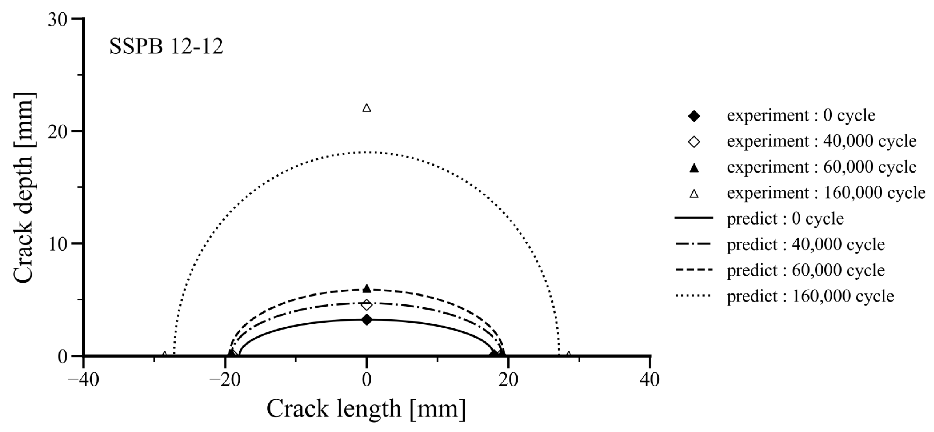
5.1. Two-Dimensional Fatigue Crack Growth

For the small aspect ratio of the semi-elliptical surface flaw (i.e., 2c/a ≤ 5), the crack grows in both the depth and length directions along with the initial shape of the flaw. Thus, crack growth was observed from both the deepest point of the flaw (point A in Figure 1b) and the intersection of the flaw with the free surface in the circumferential direction (point B in Figure 1b). This aspect of crack growth has been reported previously by Arora et al. [3].

If we control only the crack growth in the depth direction with fixed crack length, the stress intensity factor cannot be calculated due to the limitation of $f_{\mathrm{b}end}$ is given in tables in ref. [61]. Thus, crack growth in both the depth and length directions must be controlled simultaneously to predict the fatigue crack growth in pipelines with the small aspect ratio of the semi-elliptical surface flaw.

To control crack growth in both the depth and length directions simultaneously, $∆N$ was selected as the integration parameter for the finite difference method. When a fixed $∆N$ is selected, the integration of the equation becomes overly sensitive when the ligament is reduced. Thus, we used only the experimental data before the ligament was reduced severely to estimate the state. Here, we followed the procedure to predict the fatigue crack growth with the small aspect ratio of the semi-elliptical surface flaw [31].

The state model and the measurement function are given as follows:

$$C_k=C_{k-1}+{C_k(∆K_B\left(a,c\right))}^{m_k}∆N$$

(17)

$$C_{k+1}=C_k+{\omega }_{1k}$$

(18)

$$m_{k+1}=m_k+{\omega }_{2k}$$

(19)

$$y_{k1}={a_k}^{\mathrm{*}}-a_k~N(0,{{\sigma }_a}^2)$$

(20)

$$y_{k2}={c_k}^{\mathrm{*}}-c_k~N(0,{{\sigma }_c}^2)$$

(21)

where $a_k$ and $c_k$ are the state vectors of the crack depth and half-length ($a_0$ and $c_0$ are the initial crack depth and half-length), $C_k$ and $m_k$ are the random state vectors of the unknown material parameters of the fatigue law (with n number of particles), ${△K}_A(a,c)$ and ${△K}_B(a,c)$ are the stress intensity factors at positions $A$ and $B$, $w_{1k}$ and $w_{2k}$ are the zero-mean Gaussian white noise sequences, ${a_k}^{\mathrm{*}}$ and ${c_k}^{\mathrm{*}}$ are the measured crack depth and the half-length from the experiments, and $y_{k1}$ and $y_{k2}$ are the measurement functions, which are assumed to be a zero-mean Gaussian distribution with ${{\sigma }_a}^2$ and ${{\sigma }_c}^2$ variance.

• Randomly generate the initial states with n number of particles.
• For $k$ = 1, 2, ⋯, the following are carried out:

  1.

  Perform the time propagating step to obtain the next step particles using Equations (17) and (18). For Equation (17), the stress intensity factor at the deepest point of the flaw ${△K}_A(a,c)$ needs to be used, and for Equation (18), the stress intensity factor at the intersection of flaw with free surface ${△K}_B(a,c)$ needs to be used.

  2.

  Compute the relative likelihood $q_a,$ Equation (22) of each particle, conditioned on the measurement $y_{k1}$ Equation (20).

  $$q_a=P({a_k}^{\mathrm{*}}-a_k)~\frac{1}{\sqrt{2\pi }{\sigma }_a}\mathrm{e}\mathrm{x}\mathrm{p}\left(-\frac{1}{2}{\left(\frac{{a_k}^{\mathrm{*}}-a_k}{{\sigma }_a}\right)}^2\right)$$

  (22)

  3.

  Resample using the scale the relative likelihood obtained in the previous step as follows:

  $$q_{ai}=\frac{q_{ai}}{{\sum }_{j=1}^n{q}_{aj}}$$

  (23)

  4.

  Generate a set of posterior particles on the basis of the relative likelihood $q_{ai}$.

  5.

  Compute the relative likelihood $q_c$, Equation (24) of each particle, conditioned on the measurement $y_{k2}$ Equation (21).

  $$q_c=P({c_k}^{\ast }-c_k)~\frac{1}{\sqrt{2\pi }{\sigma }_c}\mathrm{e}\mathrm{x}\mathrm{p}\left(-\frac{1}{2}{\left(\frac{{c_k}^{\ast }-c_k}{{\sigma }_c}\right)}^2\right)$$

  (24)

  6.

  Resample using the scale the relative likelihood obtained in the previous step as follows:

  $$q_{ci}=\frac{q_{ci}}{{\sum }_{j=1}^n{q}_{cj}}$$

  (25)

  7.

  Generate a set of posterior particles on the basis of the relative likelihood $q_{ci}$.

In the experiments on pipes conducted by Arora et al. [3], the crack positions were measured along the crack front with different numbers of loading cycles [3]. The crack growth in both the depth and length directions can be predicted as a function of the geometrical details of the flaws and the loading using the particle filtering method with 1000 particles. The measured data (both the crack depth and length) used in each test were used for updating. In addition, a set of states $C$ and $m$ updated by the measured data was used to predict the fatigue crack growth.

The uniform distribution was considered for the initial prior distribution assuming that the prior probabilistic characteristics were not given; thus, uniform distributions were used for the initial states of $C_0~{10}^{U\left({\log }_{10}\left(1\times {10}^{-10}\right),\right({\log }_{10}\left(1\times {10}^{-8}\right)}$ and $m_0~U(1,3)$. Here, the bounds of the uniform distribution were selected according to the results of previous studies [3,4,7,8]. In addition, the COV of the relative likelihood was assumed to be 5%, and the white noises were assumed to be zero-mean normal distributions. The variations in the white noise were approximately 5% of the variance in the initial distributions, ${2.5\times 10}^{-11}$ and 0.1 for $C$ and $m$, respectively.

The fatigue crack growth predictions are shown in Figure 7, Figure 8, Figure 9 and Figure 10. Figure 7a shows the crack depth growth prediction results for SSPW 6-3, where the solid and dashed lines represent the mean values and the 90% confidence interval, respectively. Figure 7b shows the half crack length growth prediction results for SSPW 6-3. As can be seen, the crack growth in the length direction is smaller than that in the depth direction. The predictions obtained by the particle filtering method predicted crack growth in both the depth and length directions effectively. Figure 8, Figure 9 and Figure 10 show the crack growth prediction results for SSPW 6-7, SSPB 6-9, and SSPB 12-12, respectively. These figures show the results obtained with different initial crack shapes and R ratios. In the case of SSPW 6-7 in 5.8, which differs from the other results, the crack length does not grow considerably. It can also give proper results with the particle filtering method. The results shown in these figures demonstrate that the prediction framework using the particle filtering method is effective for 2D fatigue crack growth.

The crack profiles of the growing crack have been plotted. Figure 11 compares the predicted and tested crack profiles with different loading cycles for SSPW 6-7 [3]. As can be seen, the predictions in the early cycles are slightly larger than the test data. In addition, as the number of cycles increases, the prediction becomes similar to the test data. Figure 12 and Figure 13 show the crack profile prediction results for SSPB 6-9 and 12-12, respectively. As can be seen, proper results were obtained using the particle filtering method.

Crack growth with respect to 2c/a and a/t is plotted in Figure 14. As can be seen, the prediction results obtained using the particle filtering method compare well with the experimental results. Note that for the small aspect ratio of the semi-elliptical surface flaw (i.e., 2c/a ≤ 5), the crack grows in both the depth and length directions along with the initial shape of the flaw as mentioned above as shown in this figure.

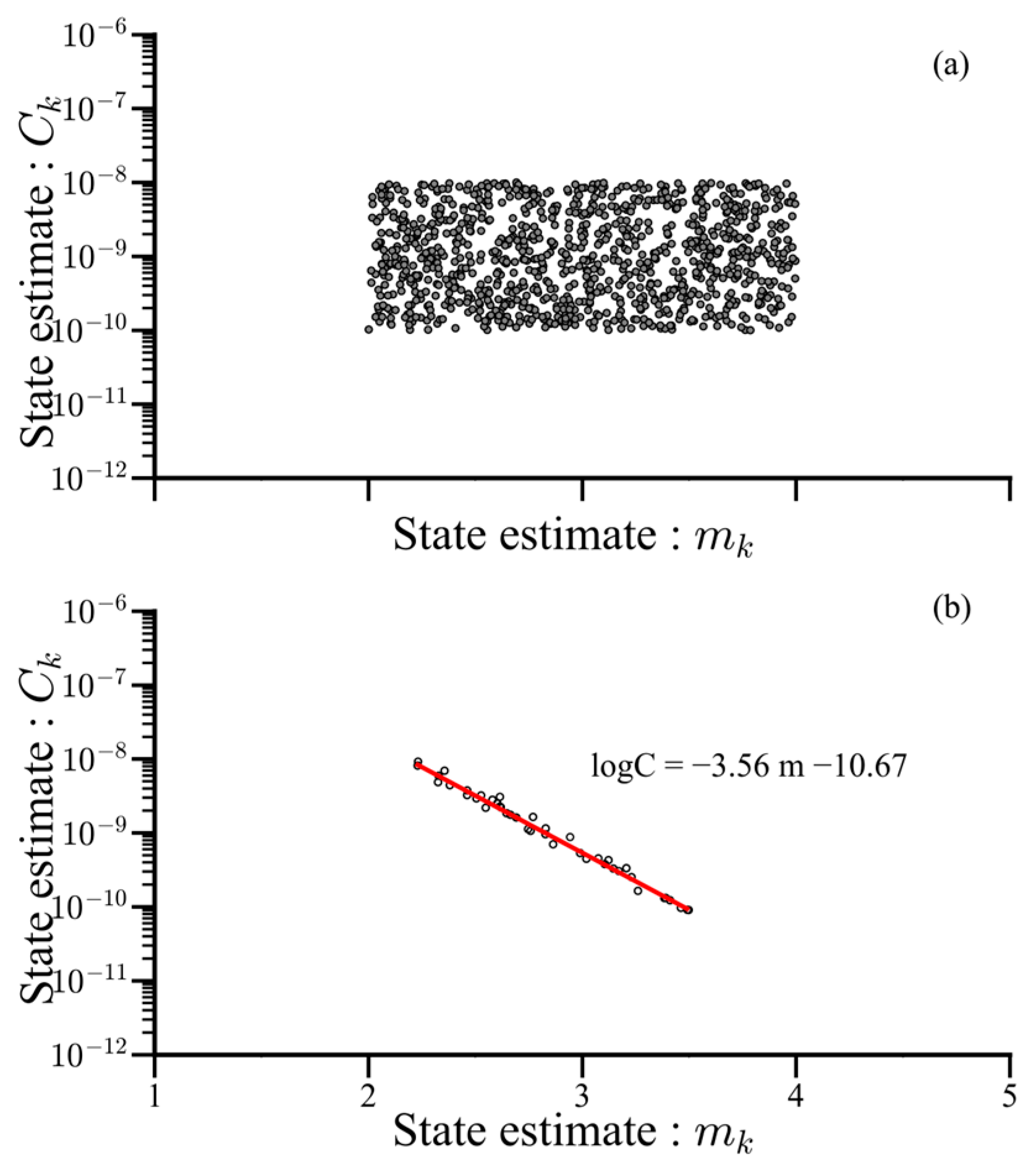
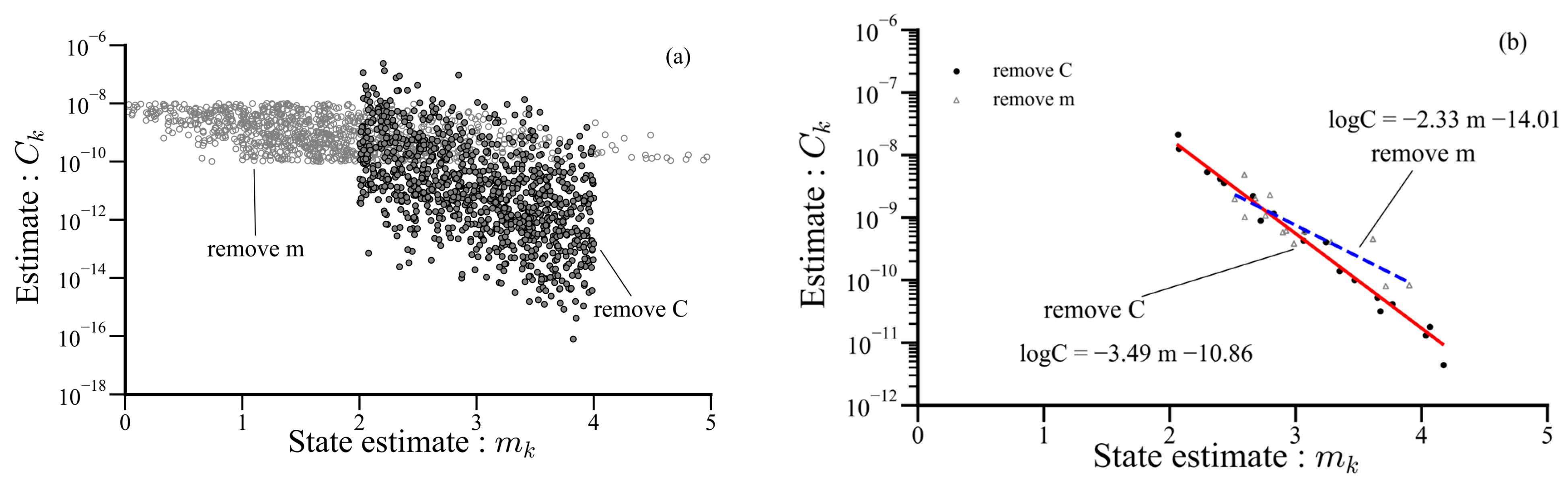
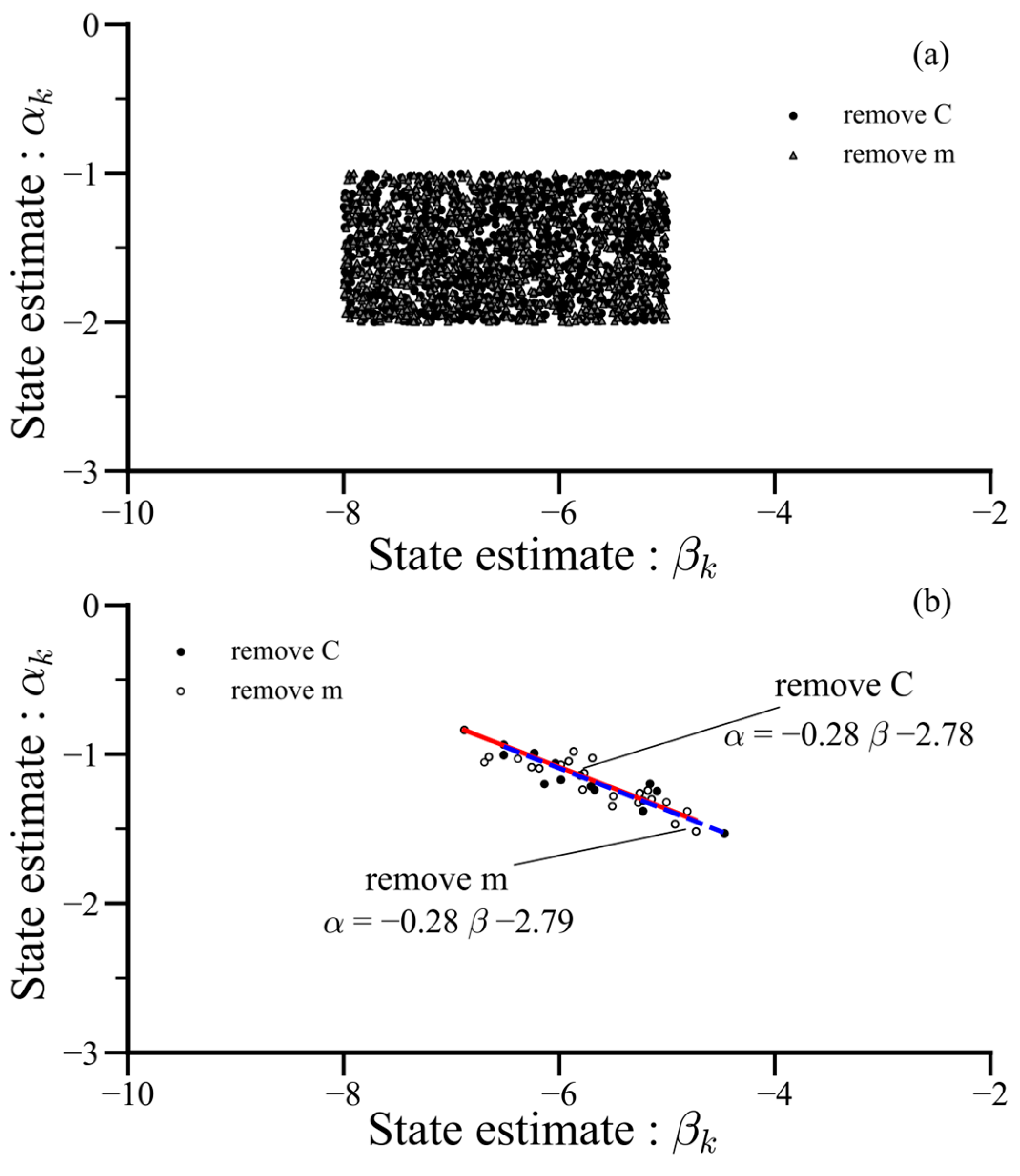
5.2. Pearson Correlation between Paris Parameters

In this section, the model’s accuracy and reliability are aimed to be enhanced by investigating and establishing the correlation between the Paris parameters $C$ and $m$, which are crucial for probabilistic fatigue crack growth predictions, using the particle filtering method. The correlation between the Paris parameters $C$ and $m$ were not considered initially, even though it has been reported that they are strongly correlated, because the prediction based on the particle filtering method can provide correlation results even though these two parameters are initially assumed to be uncorrelated [38,59,60]. In this section, we assume that these parameters are correlated initially.

As mentioned previously, the two Paris parameters are strongly correlated.

$$\mathit{log}C=\alpha m+\beta$$

(26)

Here, $\alpha$ and $\beta$ are the coefficients of the regression line under different fatigue testing conditions. As shown in

Table 3. Coefficients of the Pearson correlation relationship of Paris parameters.

Source	Material	${\mathit{\alpha }}_{\mathit{m}\mathit{i}\mathit{n}}$	${\mathit{\alpha }}_{\mathit{m}\mathit{a}\mathit{x}}$	${\mathit{\beta }}_{\mathit{m}\mathit{i}\mathit{n}}$	${\mathit{\beta }}_{\mathit{m}\mathit{a}\mathit{x}}$
Hickerson and Hertzberg (1972) [65]	Stainless steel, aluminum	−4		−16	−14.5
Benson and Edmonds (1978) [47]	1/2Cr-1/2Mo-1/4V-0.1C Steel	−1.664	−1.299	−4.776	−3.908
Cortie and Garrett (1988) [49]	1Cr-1/2Mo Steel	−3.829	−3.47	−15.59	−14.289
Bergner and Zouhar (2000) [58]	Aluminum	−0.99		−3.96
Carpinteri and Paggi (2007) [51]	Steel	−1.777	−1.742	−6.119
	Aluminum	−1.544	−1.371	−5.602
Ciavarella et al. (2008) [54]	Brittle steel	−1.190		−7.539
	Ductile steel	−1.507		−6.770
	4340 steel	−4.2		−7.43
	ASTM steel [66]	−1.62		−6.6

, it has been reported by many previous studies [47,48,49,50,51,52,58,65]. As shown in Table 3, for steel, α is in the range of −2 and −1, and β is in the range of −8 and −5 excluding extreme values.

To investigate the particle filtering method with this correlation, the experimental data where crack depth ($a$) only grows when a fixed crack length ($2c$) is used. Here, we investigated two different sets of states, i.e., (1) $m$, $\alpha$, and $\beta$ and (2) $C$, $\alpha$, and $\beta$. In the first set, the Paris parameter $C$ was removed and replaced with $\alpha$ and $\beta$ as follows:

$$N_k=N_{k-1}+\frac{∆a}{{C_k(∆K\left(a,c\right))}^{m_k}}$$

(27)

$${\alpha }_{k+1}={\alpha }_k+{\omega }_{1k}$$

(28)

$${\beta }_{k+1}={\beta }_k+{\omega }_{2k}$$

(29)

$$m_{k+1}=m_k+{\omega }_{3k}$$

(30)

$$C_{k+1}={10}^{m_{k+1}\times {\alpha }_{k+1}+{\beta }_{k+1}}$$

(31)

where ${\alpha }_k$, ${\beta }_k$, and $m_k$ are the random state vectors (with n number of particles), and $w_{1k}$, $w_{2k}$, and $w_{3k}$ are the zero-mean Gaussian white noise sequences. In the second set, the Paris parameter $m$ was removed and replaced with $\alpha$ and $\beta$ as follows:

$$N_k=N_{k-1}+\frac{∆a}{{C_k(∆K\left(a,c\right))}^{m_k}}$$

(32)

$${\alpha }_{k+1}={\alpha }_k+{\omega }_{1k}$$

(33)

$${\beta }_{k+1}={\beta }_k+{\omega }_{2k}$$

(34)

$$C_{k+1}=C_k+{\omega }_{3k}$$

(35)

$$m_{k+1}=\left(\mathit{log}{C}_{k+1}-{\beta }_{k+1}\right)/{\alpha }_{k+1}$$

(36)

In this evaluation, one set of states ($C$, $\alpha$, and $\beta$ or $m$, $\alpha$, and $\beta$) updated by the measured data was used to predict the fatigue crack growth. Here, the uniform distribution was considered for the initial prior distribution. The uniform distributions were used for the initial states of $m_0~U(2,4)$ for the first set of states, $C_0~{10}^{U\left({\log }_{10}\left(1\times {10}^{-10}\right),\right({\log }_{10}\left(1\times {10}^{-8}\right)}$ for the second set of states, ${\alpha }_0~U(-2,-1)$, and ${\beta }_0~U(-8,-5)$. In addition, the bounds of the uniform distribution were selected according to the results of previous studies, as shown in Table 3. The COV of the relative likelihood was assumed to be 5%, and the white noises in Equations (27)–(33) were assumed to be zero-mean normal distributions. The variations in the white noise were approximately 2.5% of the variance in the initial distributions, i.e., 0.075 for $m$ of the first set of states, ${1.25\times 10}^{-11}$ for $C$ of the second set of states, 0.0375 for $\alpha$, and 0.1625 for $\beta$.

Figure 15, Figure 16 and Figure 17 show the crack depth growth prediction results for PBSC8-1, PBSC8-4, and PBSC8-6, respectively. Here, the lines represent the mean values of the predicted results. As can be seen, the results obtained with the two sets of states, i.e., (1) $m$, $\alpha$, and $\beta$ and (2) $C$, $\alpha$, and $\beta$ are almost similar to those obtained with the states of $C$ and $m$. The prediction results obtained using the particle filtering method with Pearson correlation between the Paris parameters predicted the fatigue crack growth effectively.

The state estimation of these two sets of states can be compared with the results shown in Figure 5 and Figure 6. The first set of the states, i.e., $m$, $\alpha$, and $\beta$, can derive $C$ using Equation (31). In addition, the second set of the states, i.e., $C$, $\alpha$, and $\beta$, can derive $m$ using Equation (36). Figure 18 and Figure 19 show the correlation of the states for PBSC8-1 and PBSC8-4 with the two sets of states, respectively. As can be seen, the correlation of the states $C$ and $m$ from the initial distribution converges to a certain range of expected values. The relationships between $C$ and $m$ are shown in Figure 18b and Figure 19b. For PBSC8-1, the correlation is $\log C=-3.49m-10.86$ for the first set and $\log C=-2.33m-14.01$ for the second set, which is similar to $\log C=-3.57m-10.69$ from the prediction obtained while assuming that these parameters are initially not correlated. For PBSC8-4, the correlation is $\log C=-3.74m-9.92$ for the first set and $\log C=-3.52m-10.77$ for the second set, which is similar to $\log C=-3.56m-10.67$ from the prediction obtained under the assumption that these parameters are initially not correlated assuming initially uncorrelated.

The correlation between $\alpha$ and $\beta$ was also investigated. Figure 20 and Figure 21 show the correlation of the states $\alpha$ and $\beta$ for PBSC8-1 and PBSC8-4 with two different sets of states, respectively. As shown in these figures, the correlation of states $\alpha$ and $\beta$ from the initial distribution converges to a certain range of expected values (similar to $C$ and $m$). For PBSC8-1, the correlation is $\alpha =-0.28\beta -2.78$ for the first set and $\alpha =-0.28\beta -2.79$ for the second set. For PBSC8-4, the correlation is $\alpha =-0.22\beta -2.44$ for the first set and $\alpha =-0.28\beta -2.8$ for the second set. As can be seen, the two different sets exhibit nearly the same Pearson correlation.

6. Conclusions

In this study, the particle filtering method was employed to predict the effect of semi-elliptical surface flaws of pipelines on pipeline behavior.

• First, with a fixed crack length of the semi-elliptical crack, crack growth was predicted using the particle filtering method with 1000 particles for one-dimensional fatigue crack growth, focusing on crack depth. This evaluation, based on experimental data from previous studies, included various $R$ ratios and initial crack depths. The results were consistent with previous tests, indicating an effective prediction of crack growth.
• The remaining service life of each pipe was predicted based on the initial crack depth using the particle filtering method. Additionally, the simulation results showed that the Pearson correlation between the Paris parameters $C$ and $m$ converged to the expected value range, consistent with previous studies reporting a strong negative correlation. This demonstrates that the particle filtering method can effectively simulate the Pearson correlation for fatigue crack growth in a SA333 Gr.6 carbon steel pipeline, even when the parameters are initially uncorrelated.
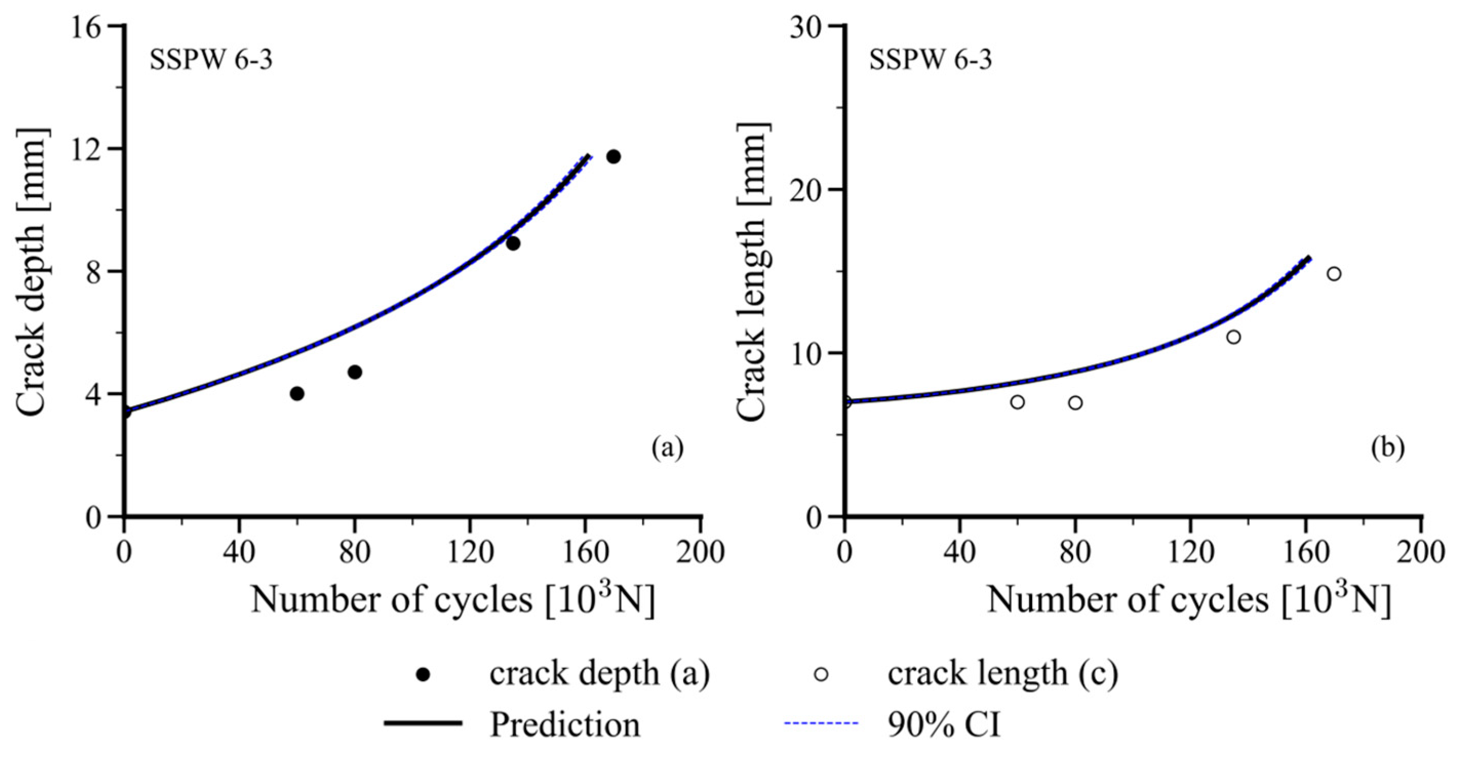
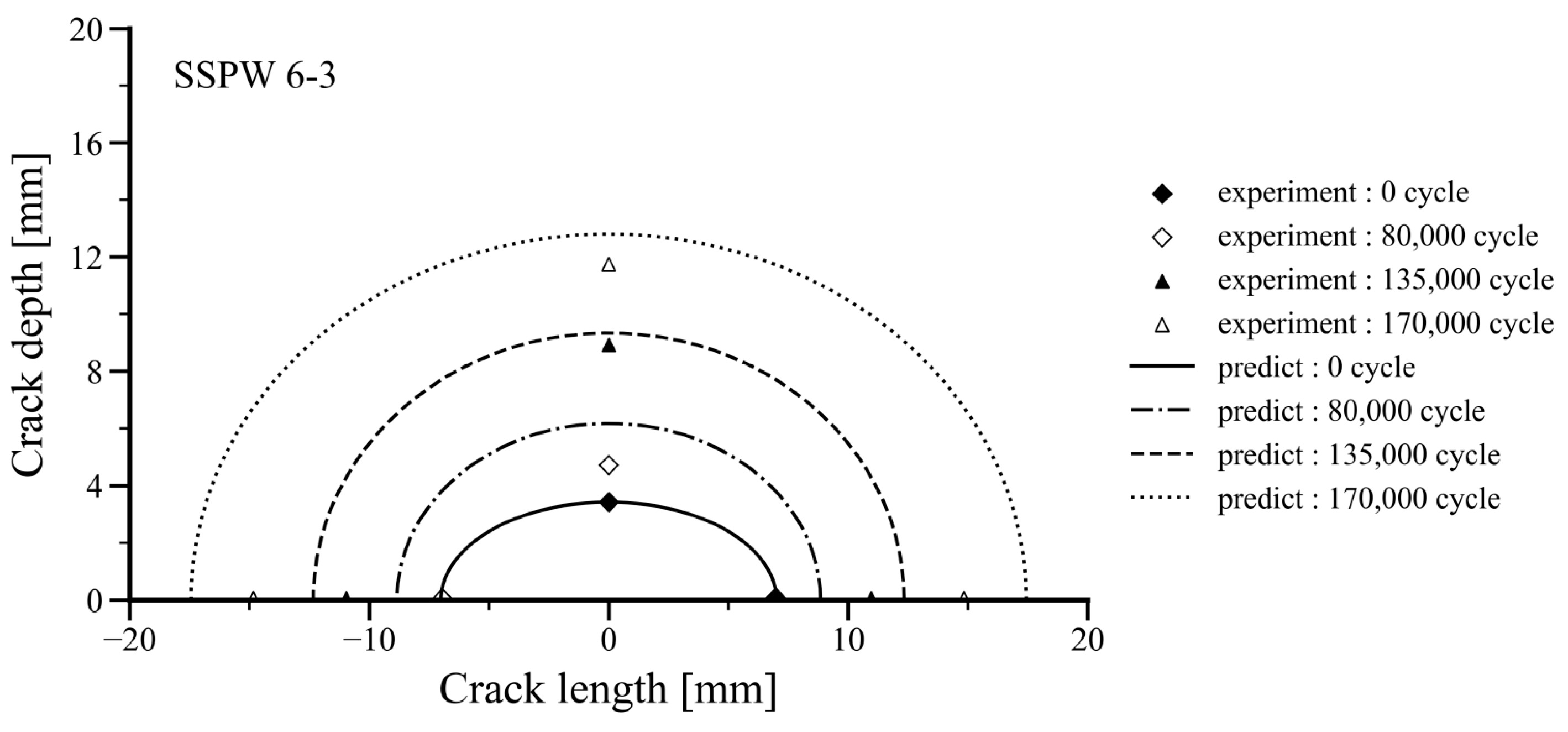
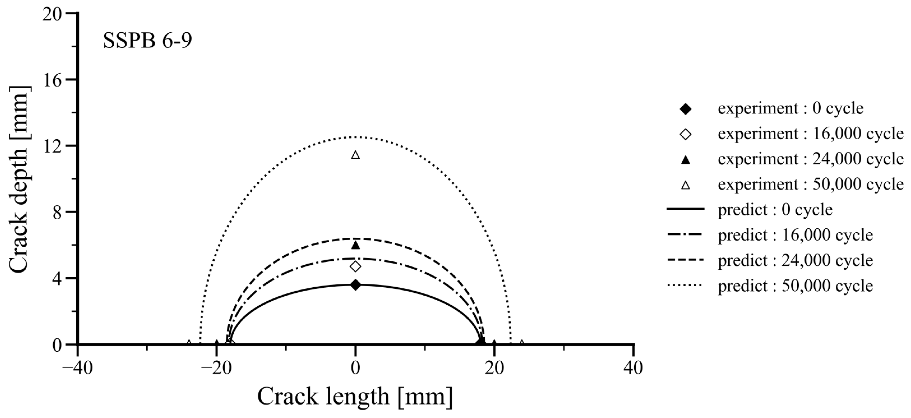
• With a small semi-elliptical surface defect aspect ratio, crack growth occurs in both depth and longitudinal directions. To predict this, the particle filtering method was combined with the finite difference method for two-dimensional fatigue crack growth. The predictions, consistent with previous studies, effectively modeled crack growth. Although initial cycle predictions were slightly larger than test data, they matched closely as the number of cycles increased, demonstrating the effectiveness of the particle filtering method in modeling two-dimensional crack growth.
• In the crack growth model considered in this study, the Pearson correlation between the Paris parameters $C$ and $m$ was predicted despite not considering their strong correlation initially. By dividing the Paris parameters into two sets of states, $m$ and $C$, we obtained fatigue crack growth prediction results similar to those using only $C$ and $m$. This indicates that the particle filtering method effectively predicted fatigue crack growth and that the correlation of each variable converged to an expected value range.
• The innovation of this research lies in applying and validating the particle filtering method for predicting fatigue crack growth in pipelines with initial flaws. This probabilistic approach continuously updates predictions with new data, enhancing accuracy and reliability. While we examined the model’s applicability based on existing experimental data, there are limitations in determining failure and critical size for practical applications. These aspects will be addressed in future work.

References

1. Ossai, C.I.; Boswell, B.; Davies, I.J. Pipeline failures in corrosive environments–A conceptual analysis of trends and effects. Eng. Fail. Anal. 2015, 53, 36–58. [Google Scholar] [CrossRef]
2. Lee, S.-J.; Cho, W.-Y.; Kim, K.-S.; Zi, G.; Yoon, Y.-C. Numerical Evaluation of Compressive Strain Capacity for API X100 Line Pipe. KSCE J. Civ. Eng. 2018, 22, 3039–3051. [Google Scholar] [CrossRef]
3. Arora, P.; Singh, P.; Bhasin, V.; Vaze, K.; Ghosh, A.; Pukazhendhi, D.; Gandhi, P.; Raghava, G. Predictions for fatigue crack growth life of cracked pipes and pipe welds using RMS SIF approach and experimental validation. Int. J. Press. Vessels Pip. 2011, 88, 384–394. [Google Scholar] [CrossRef]
4. Mittal, R.; Singh, P.; Pukazhendi, D.; Bhasin, V.; Vaze, K.; Ghosh, A. Effect of vibration loading on the fatigue life of part-through notched pipe. Int. J. Press. Vessels Pip. 2011, 88, 415–422. [Google Scholar] [CrossRef]
5. Shibata, H. On the basic research of design analysis and testing based on the failure rate for pipings and equipment under earthquake conditions. Nucl. Eng. Des. 1980, 60, 79–84. [Google Scholar] [CrossRef]
6. Shimakawa, T.; Takahashi, H.; Doi, H.; Watashi, K.; Asada, Y. Creep-fatigue crack propagation tests and the development of an analytical evaluation method for surface cracked pipe. Nucl. Eng. Des. 1993, 139, 283–292. [Google Scholar] [CrossRef]
7. Singh, P.; Vaze, K.; Bhasin, V.; Kushwaha, H.; Gandhi, P.; Murthy, D.R. Crack initiation and growth behaviour of circumferentially cracked pipes under cyclic and monotonic loading. Int. J. Press. Vessels Pip. 2003, 80, 629–640. [Google Scholar] [CrossRef]
8. Zhu, L.; Tao, X.; Cengdian, L. Fatigue strength and crack propagation life of in-service high pressure tubular reactor under residual stress. Int. J. Press. Vessels Pip. 1998, 75, 871–877. [Google Scholar] [CrossRef]
9. Luo, J.; Zhang, Y.; Li, L.; Zhu, L.; Wu, G. Fatigue failure analysis of dented pipeline and simulation calculation. Eng. Fail. Anal. 2020, 113, 104572. [Google Scholar] [CrossRef]
10. Baker, M. Delivery Order DTRS56-02-D-70036. Integrity Management Program; Research and Special Programs Administration Office of Pipeline Safety: Washington, DC, USA, 2004. [Google Scholar]
11. Vishnuvardhan, S.; Murthy, A.R.; Choudhary, A. A review on pipeline failures, defects in pipelines and their assessment and fatigue life prediction methods. Int. J. Press. Vessels Pip. 2023, 201, 104853. [Google Scholar] [CrossRef]
12. Hussain, M.; Zhang, T.; Chaudhry, M.; Jamil, I.; Kausar, S.; Hussain, I. Review of prediction of stress corrosion cracking in gas pipelines using machine learning. Machines 2024, 12, 42. [Google Scholar] [CrossRef]
13. Amerincan Petroleum Institute(API), A. 579-1/ASME FFS-1: Fitness-for-Service; American Petroleum Institute: Washington, DC, USA, 2007. [Google Scholar]
14. Meresht, E.S.; Farahani, T.S.; Neshati, J. Failure analysis of stress corrosion cracking occurred in a gas transmission steel pipeline. Eng. Fail. Anal. 2011, 18, 963–970. [Google Scholar] [CrossRef]
15. Mansor, N.; Abdullah, S.; Ariffin, A. Effect of loading sequences on fatigue crack growth and crack closure in API X65 steel. Mar. Struct. 2019, 65, 181–196. [Google Scholar] [CrossRef]
16. Li, L.; Yang, Y.; Xu, Z.; Chen, G.; Chen, X. Fatigue crack growth law of API X80 pipeline steel under various stress ratios based on J-integral. Fatigue Fract. Eng. Mater. Struct. 2014, 37, 1124–1135. [Google Scholar] [CrossRef]
17. Mohammadi Esfarjani, S.; Salehi, M. Inspection of aboveground pipeline using vibration responses. J. Pipeline Syst. Eng. Pract. 2020, 11, 04020021. [Google Scholar] [CrossRef]
18. Deng, Y.-S.; Li, L.; Yao, Z.-G.; Meng, L.-Q. Stress intensity factors and fatigue crack growth law of cracked submarine special-shaped pipe under earthquake load. Ocean Eng. 2022, 257, 111267. [Google Scholar] [CrossRef]
19. Lee, S.-J.; Zi, G.; Mun, S.; Kong, J.S.; Choi, J.-H. Probabilistic prognosis of fatigue crack growth for asphalt concretes. Eng. Fract. Mech. 2015, 141, 212–229. [Google Scholar] [CrossRef]
20. Guo, Y.; Shao, Y.; Gao, X.; Li, T.; Zhong, Y.; Luo, X. Corrosion fatigue crack growth of serviced API 5L X56 submarine pipeline. Ocean Eng. 2022, 256, 111502. [Google Scholar] [CrossRef]
21. Liu, C.; Li, B.; Cai, Y.; Chen, X. Fatigue crack propagation behaviour of pressurised elbow pipes under cyclic bending. Thin-Walled Struct. 2020, 154, 106882. [Google Scholar] [CrossRef]
22. Huang, S.; Peng, L.; Sun, H.; Li, S. Deep learning for magnetic flux leakage detection and evaluation of oil & gas pipelines: A review. Energies 2023, 16, 1372. [Google Scholar] [CrossRef]
23. Peng, D.; She, X.; Zheng, Y.; Tang, Y.; Fan, Z.; Hu, G. Research on the 3D Reverse Time Migration Technique for Internal Defects Imaging and Sensor Settings of Pressure Pipelines. Sensors 2023, 23, 8742. [Google Scholar] [CrossRef]
24. Parlak, B.O.; Yavasoglu, H.A. A comprehensive analysis of in-line inspection tools and technologies for steel oil and gas pipelines. Sustainability 2023, 15, 2783. [Google Scholar] [CrossRef]
25. Lyu, F.; Zhou, X.; Ding, Z.; Qiao, X.; Song, D. Application Research of Ultrasonic-Guided Wave Technology in Pipeline Corrosion Defect Detection: A Review. Coatings 2024, 14, 358. [Google Scholar] [CrossRef]
26. BS 7910; Guide to Methods for Assessing the Acceptability of Flaws in Metallic Structures. The British Standards Institution: London, UK, 2005.
27. CSA Z662-11; Oil and Gas Pipeline Systems. CSA Group: Toronto, ON, Canada, 2011.
28. OS-F101; Submarine Pipeline Systems. Offshore Standard: Høvik, Norway, 2000.
29. Wilkowski, G. Leak-before-break: What does it really mean? J. Press. Vessel Technol. 2000, 122, 267–272. [Google Scholar] [CrossRef]
30. Rastogi, R.; Ghosh, S.; Ghosh, A.; Vaze, K.; Singh, P. Fatigue crack growth prediction in nuclear piping using Markov chain Monte Carlo simulation. Fatigue Fract. Eng. Mater. Struct. 2017, 40, 145–156. [Google Scholar] [CrossRef]
31. Simon, D. Optimal State Estimation: Kalman, H Infinity, and Nonlinear Approaches; John Wiley & Sons: Hoboken, NJ, USA, 2006. [Google Scholar]
32. Lee, J.H.; Choi, Y.; Ann, H.; Jin, S.Y.; Lee, S.-J.; Kong, J.S. Maintenance cost estimation in PSCI girder bridges using updating probabilistic deterioration model. Sustainability 2019, 11, 6593. [Google Scholar] [CrossRef]
33. Ristic, B.; Arulampalam, S.; Gordon, N. Beyond the Kalman Filter: Particle Filters for Tracking Applications; Artech House: Norwood, MA, USA, 2003. [Google Scholar]
34. Jeong, M.C.; Lee, S.-J.; Cha, K.; Zi, G.; Kong, J.S. Probabilistic model forecasting for rail wear in seoul metro based on bayesian theory. Eng. Fail. Anal. 2019, 96, 202–210. [Google Scholar] [CrossRef]
35. Djuric, P.; Kotecha, J.; Zhang, J.; Huang, Y.; Ghirmai, T.; Bugallo, M.; Miguez, J. Particle filtering. IEEE Signal Proc. Mag. 2003, 20, 19–38. [Google Scholar] [CrossRef]
36. Cadini, F.; Zio, E.; Avram, D. Monte Carlo-based filtering for fatigue crack growth estimation. Probabilistic Eng. Mech. 2009, 24, 367–373. [Google Scholar] [CrossRef]
37. Zio, E.; Peloni, G. Particle filtering prognostic estimation of the remaining useful life of nonlinear components. Reliab. Eng. Syst. Saf. 2011, 96, 403–409. [Google Scholar] [CrossRef]
38. An, D.; Choi, J.-H.; Kim, N.H. Prognostics 101: A tutorial for particle filter-based prognostics algorithm using Matlab. Reliab. Eng. Syst. Saf. 2013, 115, 161–169. [Google Scholar] [CrossRef]
39. Wang, C.-W.; Niu, Z.-G.; Jia, H.; Zhang, H.-W. An assessment model of water pipe condition using Bayesian inference. J. Zhejiang Univ.-Sci. A 2010, 11, 495–504. [Google Scholar] [CrossRef]
40. Kim, K.; Lee, G.; Park, K.; Park, S.; Lee, W.B. Adaptive approach for estimation of pipeline corrosion defects via Bayesian inference. Reliab. Eng. Syst. Saf. 2021, 216, 107998. [Google Scholar] [CrossRef]
41. Niu, X.; He, C.; Zhu, S.-P.; Foti, P.; Berto, F.; Wang, L.; Liao, D.; Wang, Q. Defect sensitivity and fatigue design: Deterministic and probabilistic aspects in AM metallic materials. Prog. Mater. Sci. 2024, 144, 101290. [Google Scholar] [CrossRef]
42. He, J.-C.; Zhu, S.-P.; Gao, J.-W.; Liu, R.; Li, W.; Liu, Q.; He, Y.; Wang, Q. Microstructural size effect on the notch fatigue behavior of a Ni-based superalloy using crystal plasticity modelling approach. Int. J. Plast. 2024, 172, 103857. [Google Scholar] [CrossRef]
43. Liao, D.; Zhu, S.-P.; Keshtegar, B.; Qian, G.; Wang, Q. Probabilistic framework for fatigue life assessment of notched components under size effects. Int. J. Mech. Sci. 2020, 181, 105685. [Google Scholar] [CrossRef]
44. Zhou, T.; Jiang, S.; Han, T.; Zhu, S.-P.; Cai, Y. A physically consistent framework for fatigue life prediction using probabilistic physics-informed neural network. Int. J. Fatigue 2023, 166, 107234. [Google Scholar] [CrossRef]
45. Wang, L.; Zhu, S.-P.; Luo, C.; Liao, D.; Wang, Q. Physics-guided machine learning frameworks for fatigue life prediction of AM materials. Int. J. Fatigue 2023, 172, 107658. [Google Scholar] [CrossRef]
46. Wang, H.; Li, B.; Gong, J.; Xuan, F.-Z. Machine learning-based fatigue life prediction of metal materials: Perspectives of physics-informed and data-driven hybrid methods. Eng. Fract. Mech. 2023, 284, 109242. [Google Scholar] [CrossRef]
47. Benson, J.; Edmonds, D. Relationship between the parameters C and m of Paris' law for fatigue crack growth in a low-alloy steel. Scr. Metall. 1978, 12, 645–647. [Google Scholar] [CrossRef]
48. Tanaka, K.; Masuda, C.; Nishijima, S. The generalized relationship between the parameters C and m of Paris’ law for fatigue crack growth. Scr. Metall. 1981, 15, 259–264. [Google Scholar] [CrossRef]
49. Cortie, M.; Garrett, G. On the correlation between the C and m in the Paris equation for fatigue crack propagation. Eng. Fract. Mech. 1988, 30, 49–58. [Google Scholar] [CrossRef]
50. Cortie, M. The irrepressible relationship between the Paris law parameters. Eng. Fract. Mech. 1991, 40, 681–682. [Google Scholar] [CrossRef]
51. Carpinteri, A.; Paggi, M. Are the Paris’ law parameters dependent on each other? Frat. Integrità Strutt. 2007, 1, 10–16. [Google Scholar] [CrossRef]
52. Li, Y.; Wang, H.; Gong, D. The interrelation of the parameters in the Paris equation of fatigue crack growth. Eng. Fract. Mech. 2012, 96, 500–509. [Google Scholar] [CrossRef]
53. Ray, S.; Kishen, J.C. Fatigue crack propagation model for plain concrete–An analogy with population growth. Eng. Fract. Mech. 2010, 77, 3418–3433. [Google Scholar] [CrossRef]
54. Ciavarella, M.; Paggi, M.; Carpinteri, A. One, no one, and one hundred thousand crack propagation laws: A generalized Barenblatt and Botvina dimensional analysis approach to fatigue crack growth. J. Mech. Phys. Solids 2008, 56, 3416–3432. [Google Scholar] [CrossRef]
55. Carpinteri, A.; Paggi, M. Dimensional analysis and fractal modeling of fatigue crack growth. J. ASTM Int. 2011, 8, 1–13. [Google Scholar] [CrossRef]
56. Ray, S.; Kishen, J.C. Fatigue crack propagation model and size effect in concrete using dimensional analysis. Mech. Mater. 2011, 43, 75–86. [Google Scholar] [CrossRef]
57. Fathima, K.P.; Kishen, J.C. A thermodynamic framework for fatigue crack growth in concrete. Int. J. Fatigue 2013, 54, 17–24. [Google Scholar] [CrossRef]
58. Bergner, F.; Zouhar, G. A new approach to the correlation between the coefficient and the exponent in the power law equation of fatigue crack growth. Int. J. Fatigue 2000, 22, 229–239. [Google Scholar] [CrossRef]
59. An, D.; Choi, J.-H.; Kim, N.H. Identification of correlated damage parameters under noise and bias using Bayesian inference. Struct. Health Monit. 2012, 11, 293–303. [Google Scholar] [CrossRef]
60. An, D.; Choi, J.; Kim, N.H. A comparison study of methods for parameter estimation in the physics-based prognostics. In Proceedings of the 53rd AIAA/ASME/ASCE/AHS/ASC Structures, Structural Dynamics and Materials Conference 20th AIAA/ASME/AHS Adaptive Structures Conference 14th AIAA, Honolulu, HI, USA, 23–26 April 2012. [Google Scholar]
61. Andersson, P.; Bergman, M.; Brickstad, B.; Dahlberg, L.; Nilsson, F.; Sattari-Far, I. A Procedure for Safety Assessment of Components with Cracks-Handbook; Swedish Nuclear Power Inspectorate: Stockholm, Sweden, 1999. [Google Scholar]
62. Kitagawa, G. A self-organizing state-space model. J. Am. Stat. Assoc. 1998, 93, 1203–1215. [Google Scholar] [CrossRef]
63. Dowd, M.; Joy, R. Estimating behavioral parameters in animal movement models using a state-augmented particle filter. Ecology 2011, 92, 568–575. [Google Scholar] [CrossRef]
64. Simon, D. Kalman h-infinity and nonlinear approaches. In Optimal State Estimation; John Wiley & Sons: Hoboken, NJ, USA, 2006. [Google Scholar]
65. Hickerson, J.; Hertzberg, R. The role of mechanical properties in low-stress fatigue crack propagation. Metall. Mater. Trans. B 1972, 3, 179–189. [Google Scholar] [CrossRef]
66. ASTM E399-90; Standard Test Method for Plane-Strain Fracture Toughness of Metallic Materials. American Society for Testing and Materials (ASTM): West Conshohocken, PA, USA, 1997.
Figure 1. Pipeline cross-sections with circumferential flaws: (a) circumferential embedded flaw and (b) circumferential surface flaw.
Buildings 14 01775 g001
Figure 2. Intuitive schematic description of the particle filtering method.
Buildings 14 01775 g002
Figure 3. The predicted fatigue crack growth data [7] in the depth direction: (a) a 0 = 5.5   m m , (b) a 0 = 3.0   m m , and (c) a 0 = 2.0   m m .
Buildings 14 01775 g003
Figure 4. The predicted remaining service life [7]: (a) a 0 = 5.5   m m , (b) a 0 = 3.0   m m , and (c) a 0 = 2.0   m m .
Buildings 14 01775 g004
Figure 5. Pearson correlation of states C and m for PBSC8-1 [7] at (a) initial states and after and (b) the fifth updating.
Buildings 14 01775 g005
Figure 6. Pearson correlation of states C and m for PBSC8-4 [7] at (a) initial states and after and (b) the fifth updating.
Buildings 14 01775 g006
Figure 7. The predicted fatigue crack growth data for SSPW 6-3 [3]: (a) crack depth and (b) half crack length.
Buildings 14 01775 g007
Figure 8. The predicted fatigue crack growth data for SSPW 6-7 [3]: (a) crack depth and (b) half crack length.
Buildings 14 01775 g008
Figure 9. The predicted fatigue crack growth data for SSPB 6-9 [3]: (a) crack depth and (b) half crack length.
Buildings 14 01775 g009
Figure 10. The predicted fatigue crack growth data for SSPB 12-12 [3]: (a) crack depth and (b) half crack length.
Buildings 14 01775 g010
Figure 11. The prediction of crack profiles with different cycles for SSPW 6-3 [3].
Buildings 14 01775 g011
Figure 12. The prediction of crack profiles with different cycles for SSPB 6-9 [3].
Buildings 14 01775 g012
Figure 13. The prediction of crack profiles with different cycles for SSPB 12-12 [3].
Buildings 14 01775 g013
Figure 14. Comparison of 2c/a vs. a/t curves in ref. [3] in which the lines represent predicted mean values, and the symbols represent the measured data.
Buildings 14 01775 g014
Figure 15. The predicted fatigue crack growth data for PBSC8-1 [7].
Buildings 14 01775 g015
Figure 16. The predicted fatigue crack growth data for PBSC8-4 [7].
Buildings 14 01775 g016
Figure 17. The predicted fatigue crack growth data for PBSC8-6 [7].
Buildings 14 01775 g017
Figure 18. Pearson correlation of states C and m for PBSC8-1 [7] with two different sets of states (1) m, α, and β and (2) C, α, and β at (a) initial states and after and (b) the fifth updating.
Buildings 14 01775 g018
Figure 19. Pearson correlation of states C and m for PBSC8-4 [7] with two different sets of states (1) m, α, and β and (2) C, α, and β at (a) initial states and after and (b) the fifth updating.
Buildings 14 01775 g019
Figure 20. Pearson correlation of states α and β for PBSC8-1 [7] with two different sets of states (1) m, α, and β and (2) C, α, and β at (a) initial states and after and (b) the fifth updating.
Buildings 14 01775 g020
Figure 21. Pearson correlation of states α and β for PBSC8-4 [7] with two different sets of states at (1) m, α, and β and (2) C, α, and β at (a) initial states and after and (b) the fifth updating.
Buildings 14 01775 g021