
The Simplified Method of Head Stiffness Considering Semi-Rigid Behaviors of Deep Foundations in OWT Systems

Abstract
:1. Introduction
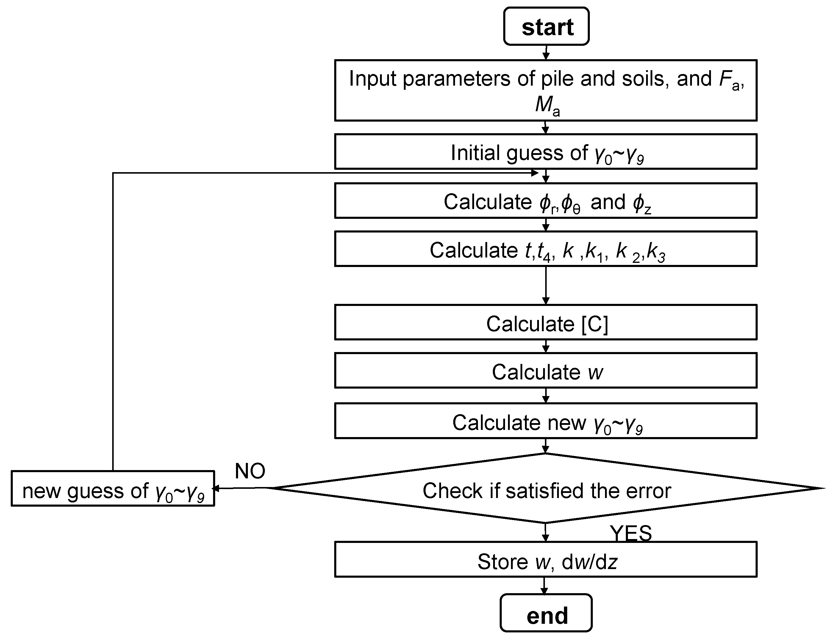
2. Methodology
2.1. Energy-Based Variational Method
2.2. Soil Conditions
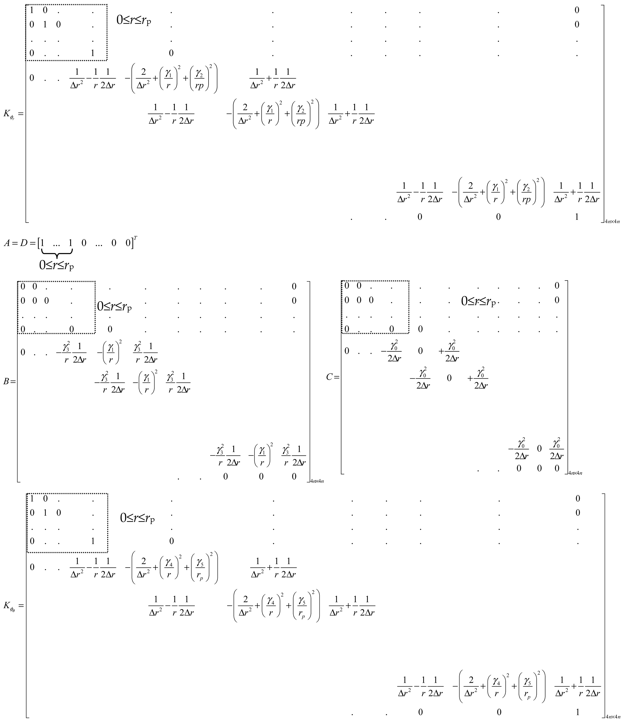
2.3. Governing Differential Equations of the Beam and Soils
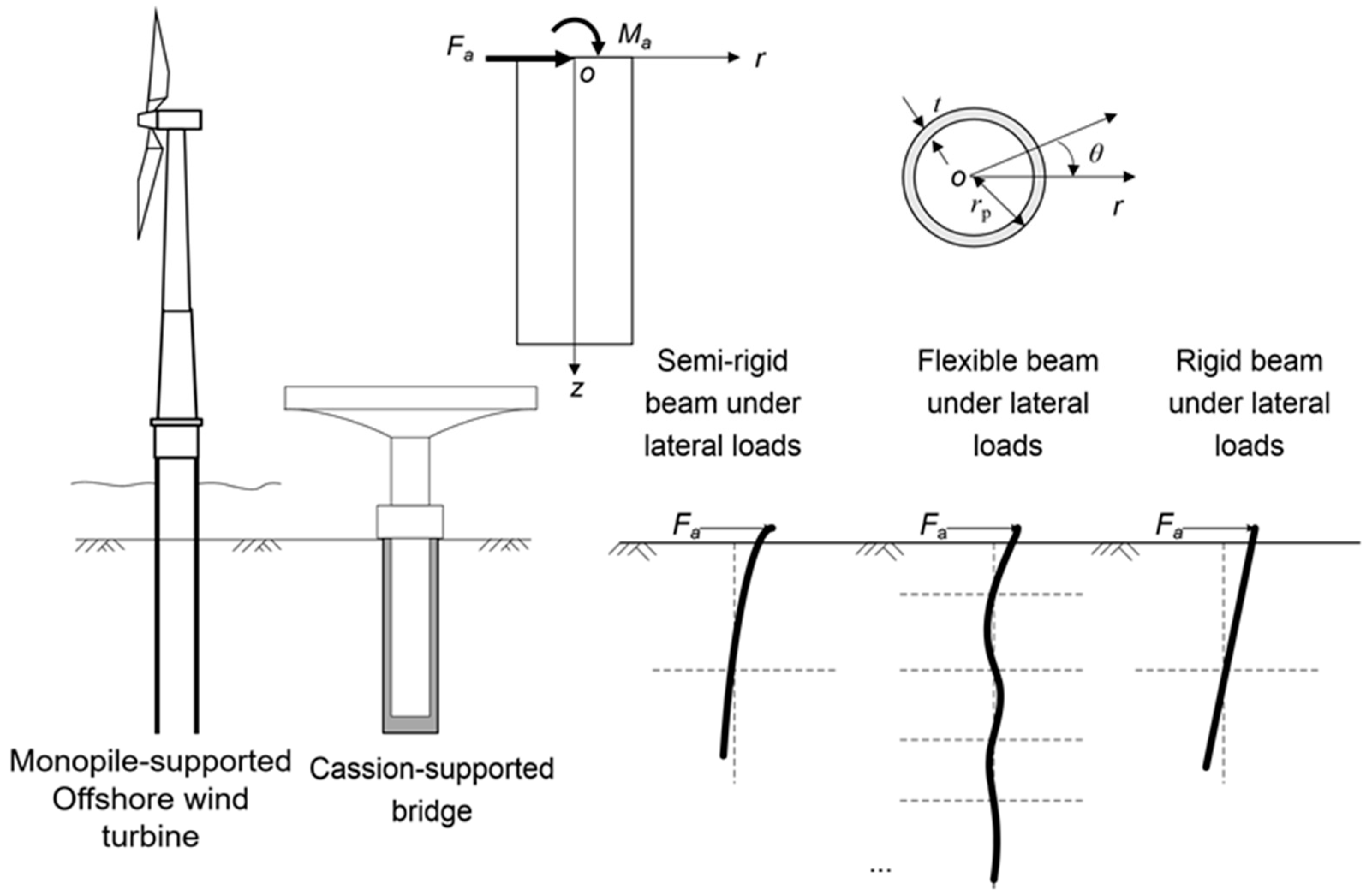
2.4. Modeling Cases
3. Results and Discussion
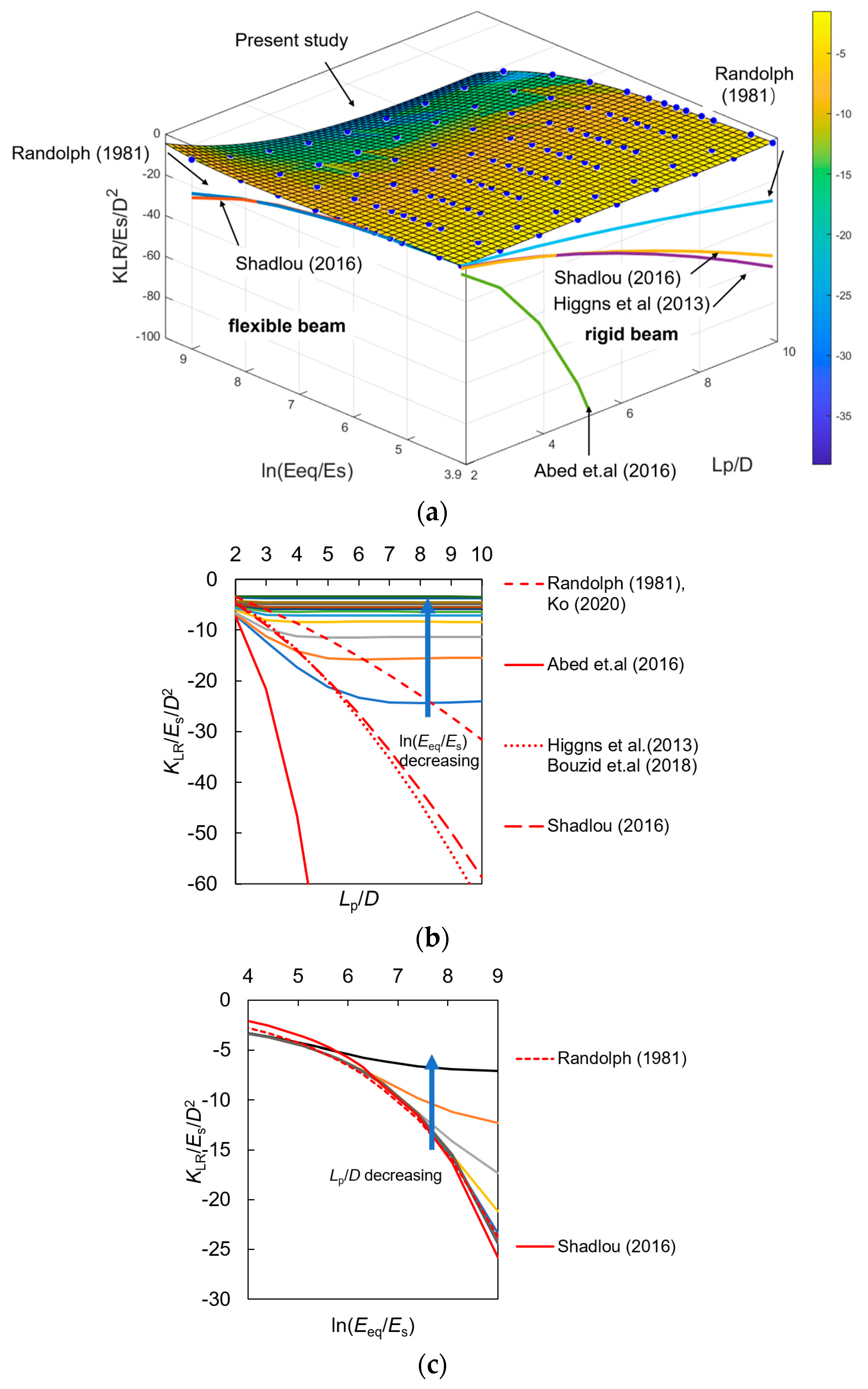
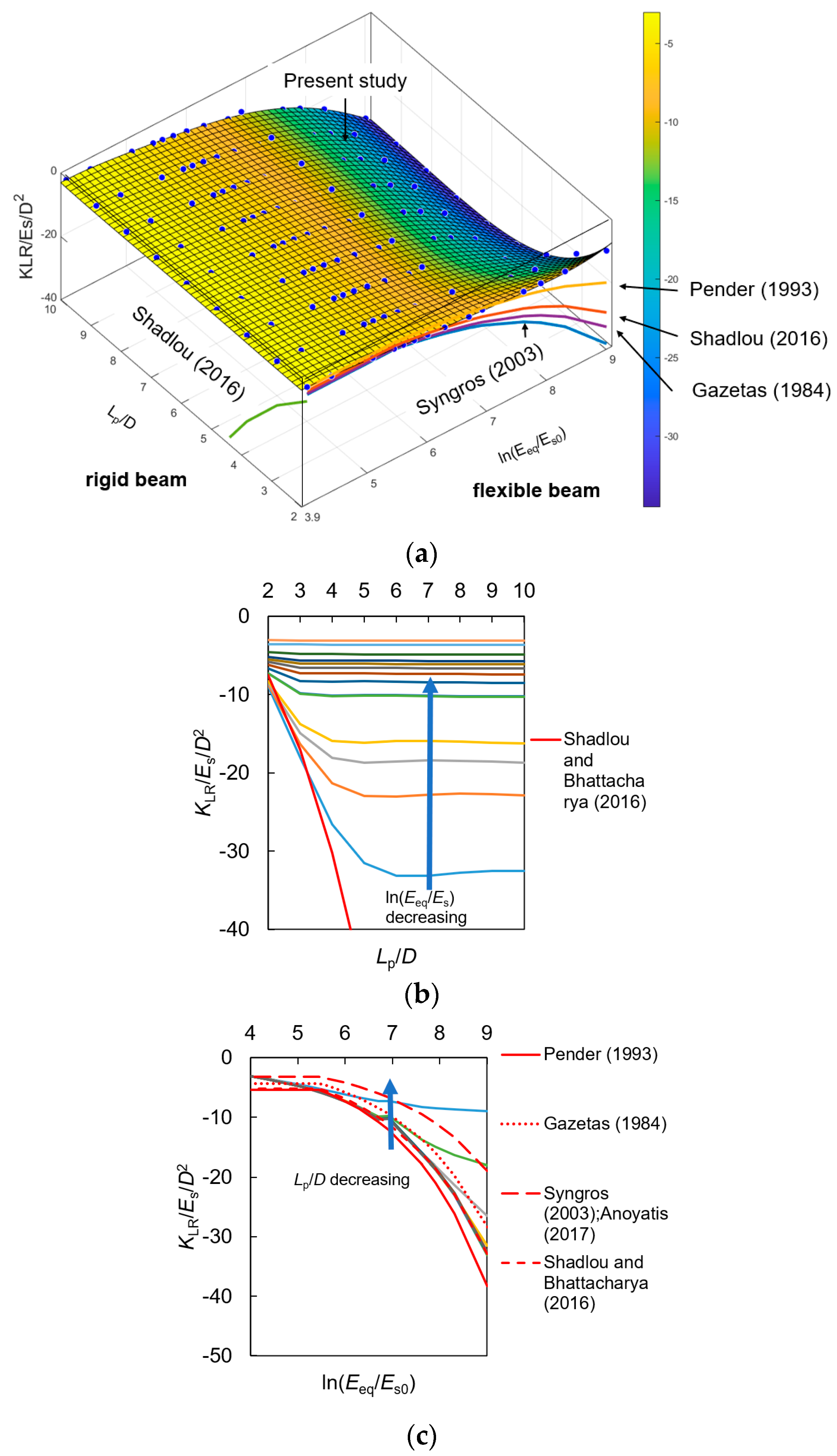
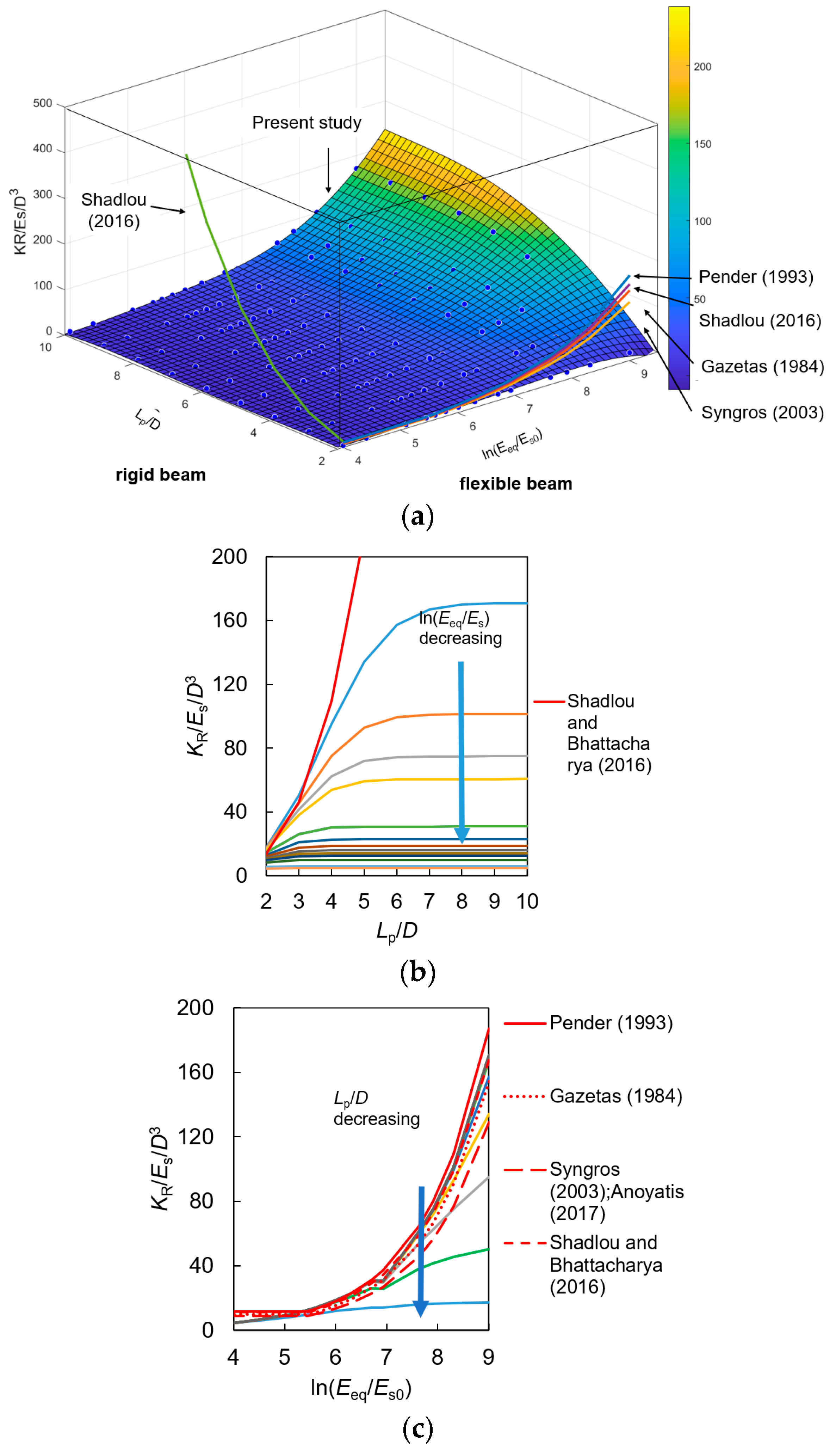
3.1. Validation of the Analysis Compared against Different Methods
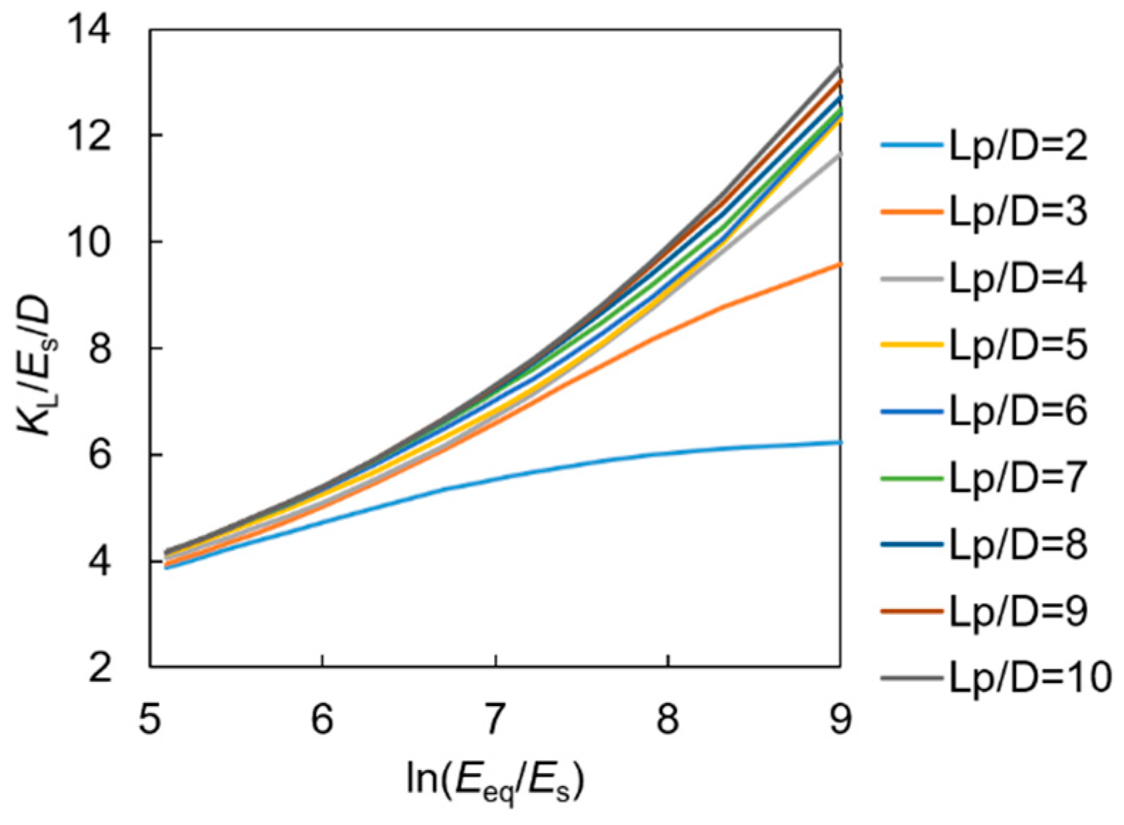
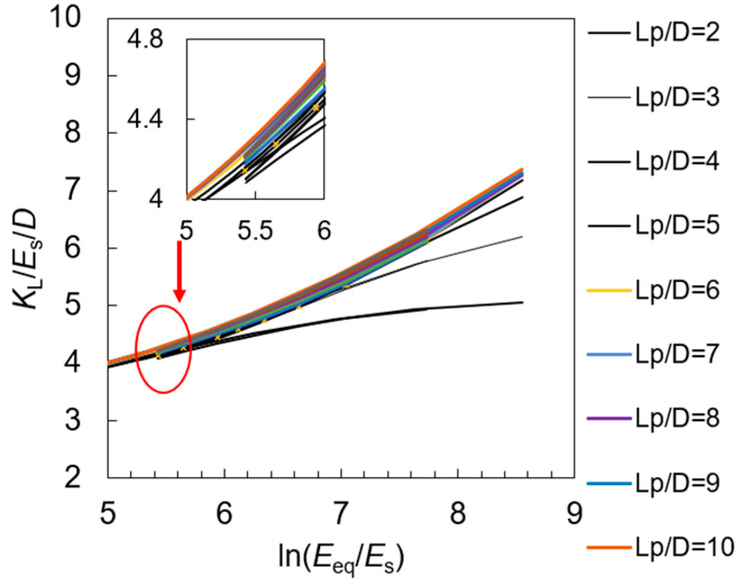
3.2. Parameter Analysis
3.3. The Equations of Stiffness of Pile-Head Springs
4. Application of the Methodology
4.1. The Lateral Deflection and Rotation of Caissons for Serviceability Limit State Calculations
4.2. The Natural Frequency of OWT Considering the SSI Effect
5. Conclusions
Author Contributions
Funding
Data Availability Statement
Acknowledgments
Conflicts of Interest
Notation
| D | the outer diameter of caisson |
| dw/dz | the rotation of the beam section |
| Eeq | the equivalent Young’s modulus of the beam |
| Ep | the Young’s modulus of the beam |
| Esi | the elastic modulus of the ith layer of soil |
| Es0 | the initial value of soil elastic modulus |
| Fa | the lateral force at the head of beam |
| Ip | the second moment of inertia of cross-section |
| KL | lateral stiffness |
| KR | rocking stiffness |
| KLR | cross-coupling stiffness |
| Lp | the embedment depth of beam |
| mRNA | mass of rotor-nacelle assembly (kg) |
| Ma | the moment at the head of beam |
| R2 | a coefficient of determination |
| rp | the radius of the beam |
| t | the wall thickness of beam |
| uz | the vertical displacement |
| w | the lateral displacement of the beam central line |
| α | the index of the function |
| γ | the relative stiffness of the pile and soil |
| Ω | the soil domain that participates in the structure-soil interaction |
| ϕ | the shear rotation of the plane section |
| κ | the shear correction factor |
| σpq | the stress in soil domain |
| εpq | the strain in soil domain |
| λsi, Gsi | the Lame’s constants of the ith layer of the multilayered continuum |
| vsi | the Poisson’s ratio of the ith layer of soil |
| ϕr | dimensionless decay functions of the displacement components in the r-directions |
| ϕθ | dimensionless decay functions of the displacement components in the θ-directions |
| ϕz | dimensionless decay functions of the displacement components in the z-directions |
Appendix A
Appendix B
Appendix C

References
- Qin, W.; Cai, S.; Dai, G.; Wang, D.; Chang, K. Soil Resistance during Driving of Offshore Large-Diameter Open-Ended Thin-Wall Pipe Piles Driven into Clay by Impact Hammers. Comput. Geotech. 2023, 153, 105085. [Google Scholar] [CrossRef]
- Qin, W.; Cai, S.; Dai, G.; Wei, H. Analytical solutions of soil plug behaviors in open-ended pile driven by impact load. Acta Geotech. 2023, 18, 4183–4194. [Google Scholar] [CrossRef]
- Qin, W.; Gao, J.; Chang, K.; Dai, G.; Wei, H. Set-up effect of large-diameter open-ended thin-walled pipe piles driven in clay. Comput. Geotech. 2023, 159, 105459. [Google Scholar] [CrossRef]
- Wu, J.-S.; Hsu, S.-H. A unified approach for the free vibration analysis of an elastically supported immersed uniform beam carrying an eccentric tip mass with rotary inertia. J. Sound Vib. 2006, 291, 1122–1147. [Google Scholar] [CrossRef]
- Galvín, P.; Romero, A.; Solís, M.; Domínguez, J. Dynamic characterisation of wind turbine towers account for a monopile foundation and different soil conditions. Struct. Infrastruct. Eng. 2016, 13, 942–954. [Google Scholar] [CrossRef]
- Wang, P.; Zhao, M.; Du, X.; Liu, J.; Xu, C. Wind, wave and earthquake responses of offshore wind turbine on monopile foundation in clay. Soil Dyn. Earthq. Eng. 2018, 113, 47–57. [Google Scholar] [CrossRef]
- Arany, L.; Bhattacharya, S.; John, M.; Hogan, S.J. Design of monopiles for offshore wind turbines in 10 steps. Soil Dyn. Earthq. Eng. 2017, 92, 126–152. [Google Scholar] [CrossRef]
- Subhamoy, B. Design of Foundations for Offshore Wind Turbines; John Wiley & Sons Ltd.: West Sussex, UK, 2017. Available online: https://lccn.loc.gov/2018046931 (accessed on 16 February 2024).
- Hu, Q.; Han, F.; Prezzi, M.; Salgado, R.; Zhao, M. Lateral load response of large-diameter monopiles in sand. Géotechnique 2021, 72, 1035–1050. [Google Scholar] [CrossRef]
- Hu, Q.; Han, F.; Prezzi, M.; Salgado, R.; Zhao, M. Finite-element analysis of the lateral load response of monopiles in layered sand. J. Geotech. Geoenviron. Eng. 2022, 148, 04022001. [Google Scholar] [CrossRef]
- Bergfelt, A. The axial and lateral loading bearing capacity, and failure by buckling of piles in soft clay. In Proceedings of the 4th International Conference on Soil Mechanics and Foundation Engineering, London, UK, 12–14 August 1957; Volume 2, pp. 8–19. [Google Scholar]
- Thomas, G. Determination of Spring Constant, Term Project; Rensselaer Polytechnic Institute: Troy, NY, USA, 1978. [Google Scholar]
- Randolph, M. The response of flexible piles to lateral loading. Geotechnique 1981, 2, 247–259. [Google Scholar] [CrossRef]
- Poulos, H.; Davis, E. Pile Foundation Analysis and Design; Rainbow-Bridge Book Co.: Landon, UK, 1980. [Google Scholar]
- Barber, E.S. Discussion to paper by S. M. Gleser. ASTM Spec. Tech. Publ. 1953, 154, 96–99. [Google Scholar]
- Budhu, M.; Davies, G. Analysis of Laterally Loaded Piles in Soft Clays. J. Geotech. Eng. 1988, 114, 21. [Google Scholar] [CrossRef]
- Pender, M.J. ASeismic Pile Foundation Design Analysis. Bull. N. Z. Natl. Soc. Earthq. Eng. 1993, 26, 49–161. [Google Scholar] [CrossRef]
- Gazetas, G. Seismic response of end-bearing single piles. Int. J. Soil Dyn. Earthq. Eng. 1984, 3, 82–93. [Google Scholar] [CrossRef]
- Higgins, W.; Vasquez, C.; Basu, D.; Griffiths, D.V. Elastic solutions for laterally loaded piles. J. Geotech. Geoenviron. Eng. 2013, 139, 1096–1103. [Google Scholar] [CrossRef]
- Shadlou, M.; Bhattacharya, S. Dynamic stiffness of monopiles supporting offshore wind turbine generators. Soil Dyn. Earthq. Eng. 2016, 8, 15–32. [Google Scholar] [CrossRef]
- Aissa, M.; Bouzid, D.A.; Bhattacharya, S. Monopile head stiffness for serviceability limit state calculations in assessing the natural frequency of offshore wind turbines. Int. J. Geotech. Eng. 2017, 6, 267–283. [Google Scholar] [CrossRef]
- Anoyatis, G.; Lemnitzer, A. Dynamic pile impedances for laterally-loaded piles using improved Tajimi and Winkler formulations. Soil Dyn. Earthq. Eng. 2017, 92, 279–297. [Google Scholar] [CrossRef]
- Rao, S.S. Vibration of Continuous Systems; John Wiley & Sons, Inc.: Hoboken, NJ, USA, 2007. [Google Scholar]
- Ko, Y.; Li, Y. Response of a scale-model pile group for a jacket foundation of an offshore wind turbine in liquefiable ground during shaking table tests. Earthq. Eng. Struct. Dyn. 2020, 49, 1682–1701. [Google Scholar] [CrossRef]
- European Committee for Standardization. Eurocode 8: Design of Structures for Earthquake Resistance—Part 5: Foundations, Retaining Structures and Geotechnical Aspects; European Committee for Standardization: Brussels, Belgium, 2003. [Google Scholar]
- Syngros, C. Seismic Response of Piles and pile-Supported Bridge Piers Evaluated through Case Histories. Ph.D. Thesis, City University of New York, New York, NY, USA, 2004. [Google Scholar]
- Carter, J.; Kulhawy, F. Analysis of laterally loaded shafts in rock. J. Geotech. Eng. 1992, 118, 839–855. [Google Scholar] [CrossRef]
- Bouzid, D.A.; Bhattacharya, S.; Otsmane, L. Assessment of natural frequency of installed offshore wind turbines using nonlinear finite element model considering soil-monopile interaction. J. Rock Mech. Geotech. Eng. 2018, 10, 333–346. [Google Scholar] [CrossRef]
- Abed, Y.; Bouzid, D.A.; Bhattacharya, S. Static impedance functions for monopiles supporting offshore wind turbines in nonhomogeneous soils emphasis on soil/monopile interface characteristics. Earthq. Struct. 2016, 10, 1143–1179. [Google Scholar] [CrossRef]
- Salgado, R.; Tehrani, F.S.; Prezzi, M. Analysis of laterally loaded pile groups in multilayered elastic soil. Comput. Geotech. 2014, 62, 136–153. [Google Scholar] [CrossRef]
- Han, F. Axial and Lateral Resistance of Non-Displacement Piles. Ph.D. Thesis, Purdue University, West Lafayette, IN, USA, 2017. [Google Scholar]
- Han, F.; Prezzi, M.; Salgado, R. Energy-based solutions for non-displacement piles subjected to lateral loads. Int. J. Geomech. 2017, 17, 04017104. [Google Scholar] [CrossRef]
- Byrne, B.W.; Burd, H.J.; Houlsby, G.T. New Design Methods for Large Diameter Piles under Lateral Loading for Offshore Wind Applications. In Proceedings of the Third International Symposium on Frontiers in Offshore Geotechnics ISFOG, Oslo, Norway, 10–12 June 2015. [Google Scholar]
- Byrne, B.W.; Mcadam, R.A.; Burd, H.J. Field testing of large diameter piles under lateral loading for offshore wind applications. In Proceedings of the XVI European Conference on Soil Mechanics and Geotechnical Engineering (ECSMGE), Edinburg, UK, 13–17 September 2016; pp. 1255–1260. [Google Scholar]
- Gupta, B.K.; Basu, D. Applicability of Timoshenko, Euler–Bernoulli and rigid beam theories in the analysis of laterally loaded monopiles and piles. Géotechnique 2018, 9, 772–785. [Google Scholar] [CrossRef]
- Gupta, B.K.; Basu, D. Offshore wind turbine monopile foundations: Design perspectives. Ocean Eng. 2020, 213, 107514. [Google Scholar] [CrossRef]
- Gupta, B.K. Dynamic pile-head stiffness of laterally loaded end-bearing pile in linear viscoelastic soil—A comparative study. Comput. Geotech. 2022, 145, 104654. [Google Scholar] [CrossRef]
- Cao, G.; Hian, S.; Ding, X. Horizontal static for OWT monopiles based on Timoshenko beam theory. Int. J. Geomech. 2023, 23, 04023202. [Google Scholar] [CrossRef]
- Li, X.; Dai, G.; Zhang, F.; Gong, W. Energy-Based analysis of laterally loaded caissons with large diameters under small-strain conditions. Int. J. Geomech. 2022, 22, 05022005. [Google Scholar] [CrossRef]
- Li, X.; Dai, G. Closure to “Energy-Based Analysis of Laterally Loaded Caissons with Large Diameters under Small-Strain Conditions”. Int. J. Geomech. 2023, 23, 07023008. [Google Scholar] [CrossRef]
- Li, X.; Dai, G.; Zhu, M.; Zhu, W.; Zhang, F. Investigation of the soil deformation around late-rally loaded deep foundations with large diameters. Acta Geotech. 2023, 19, 2293–2314. [Google Scholar] [CrossRef]
- Li, X.; Dai, G.; Zhu, M.; Wang, L.; Liu, H. A Simplified Method for Estimating the Initial Stiffness of Monopile—Soil Interaction Under Lateral Loads in Offshore Wind Turbine Systems. China Ocean Eng. 2023, 37, 165–174. [Google Scholar] [CrossRef]
- Li, X.; Zhu, M.; Dai, G.; Wang, L.; Liu, J. Interface Mechanical Behavior of Flexible Piles Under Lateral Loads in OWT Systems. China Ocean Eng. 2023, 3, 484–494. [Google Scholar] [CrossRef]
- Bhattacharya, S.; Carrington, T.; Aldridge, T. Observed increases in offshore piledriving resistance. Proc. Inst. Civ. Eng.—Geotech. Eng. 2009, 162, 71–80. [Google Scholar] [CrossRef]
- Skempton, A.W.; Henkel, D.J. Tests on London Clay fromDeepBorings at Paddington, Victoria, and the South Bank. In Proceedings of the 4th International Conference on Soil Mechanics and Foundation Engineering, London, UK, 12–14 August 1957; Volume 1, pp. 100–106. [Google Scholar]
- Ward, W.H.; Marsland, A.; Samuels, S.G. Properties of the London Clay at the Ashford Common Shaft: In-Situ and Undrained Strength Tests. Geotechnique 1965, 15, 321–344. [Google Scholar] [CrossRef]
- Burland, J.B.; Lord, J.A. The Load-Deformation Behavior of the Middle Chalk at Mundford, Norfolk: A Comparison between Full Scale Performance and In-Situ Laboratory Measurements, Building Research Station CP. 1969. Available online: https://eurekamag.com/research/018/258/018258882.php (accessed on 16 February 2024).
- Butler, F.G. Heavily Over-Consolidated Clays. In BGS Conference on Settlement of Structures; Wiley: London, UK, 1974; pp. 531–578. Available online: http://www.geosolve.co.uk/refs/Butler_F_G_1975.pdf (accessed on 16 February 2024).
- Hobbs, N.B. Factors Affecting the Prediction of Settlement on Rock with Particular Reference to Chalk and Trias. In BGS Conference on Settlement of Structures; Wiley: London, UK, 1974; p. 579-560. [Google Scholar]
- Selvadurai, P. The Analytical Method in Geomechanics. Appl. Mech. Rev. 2007, 60, 87–106. [Google Scholar] [CrossRef]
- Malekjafarian, A.; Jalilvand, S.; Doherty, P.; Igoe, D. Foundation damping for monopile supported offshore wind turbines: A review. Mar. Struct. 2021, 77, 102937. Available online: https://www.sciencedirect.com/science/article/pii/S0951833921000058 (accessed on 16 February 2024). [CrossRef]
- Jalbi, S.; Shadlou, M.; Bhattacharya, S. Impedance functions for rigid skirted caissons supporting offshore wind turbines. Ocean Eng. 2018, 150, 21–35. [Google Scholar] [CrossRef]
- ABAQUS. Abaqus Analysis User’s Manual: ABAQUS 6.15; SIMULIA: Johnston, RI, USA, 2018. [Google Scholar]
- Laszlo, A.; Bhattacharya, S.; Macdonald, J.H.G.; Hogan, S.J. Closed-form solution of Eigen frequency of monopile supported offshore wind turbines in deeper waters incorporating stiffness of substructure and SSI. Soil Dyn. Earthq. Eng. 2016, 83, 18–32. [Google Scholar] [CrossRef]
- The MathWorks Inc. Optimization Toolbox Version: (R2018b); The MathWorks Inc.: Natick, MA, USA, 2018; Available online: https://www.mathworks.com (accessed on 16 February 2024).


| Source | KL, KR and KLR (If Have) | Constant Value | Beam and Soil Material | |||
|---|---|---|---|---|---|---|
| KL | KLR | KR | Others | |||
| Randolph [13], Ko [24] | KL: KLR: KR: | a1 = 3.147 b1 = 1/7 | a2 = −0.5311 b2 = 3/7 | a3 = 0.2458 b3 = 5/7 | Es0 is the initial value of soil elastic modulus | The Semi-infinite beam in homogeneous and linear inhomogeneous soils (Triangular-linear strain element) |
| Pender [17] | a1 = 1.285 b1 = 0.188 | a2 = −0.3075 b2 = 0.47 | a3 = 0.18125 b3 = 0.738 | f(vs) = 1 m* is the equivalent ratio of shear modulus, m* = dGs/dz(1 + 0.75νs) | The Semi-infinite beam in homogeneous soil | |
| a1 = 0.85 b1 = 0.29 | a2 = −0.24 b2 = 0.53 | a3 = 0.15 b3 = 0.77 | The Semi-infinite beam in linear inhomogeneous homogeneous soil | |||
| a1 = 0.735 b1 = 0.33 | a2 = −0.27 b2 = 0.55 | a3 = 0.1725 b3 = 0.776 | The Semi-infinite beam in parabolic inhomogeneous soil | |||
| Gazetas [18] and Eurocode 8 Part 5 [25] | a1 = 1.08 b1 = 0.21 | a2 = −0.22 b2 = 0.50 | a3 = 0.16 b3 = 0.75 | The Semi-infinite beam in homogeneous soil | ||
| a1 = 0.60 b1 = 0.35 | a2 = −0.17 b2 = 0.60 | a3 = 0.14 b3 = 0.80 | The Semi-infinite beam in linear inhomogeneous soil | |||
| a1 = 0.79 b1 = 0.28 | a2 = −0.24 b2 = 0.53 | a3 = 0.15 b3 = 0.77 | The Semi-infinite beam in parabolic inhomogeneous soil | |||
| a1 = 0.1967 m* b1 = 18 | a2 = −0.3472 m* b2 = 0.43 | a3 = 0.2083 m* b3 = 0.72 | - | |||
| a1=0.1967 m* b1 = 33 | a2=−0.3472 m* b2 = 0.54 | a3=0.2083 m* b3 = 0.78 | - | |||
| Syngros [26]; Anoyatis [22] | a1 = 1.24 b1 = 0.18 | a2 = −0.21 b2 = 0.50 | a3 = 0.15 b3 = 0.75 | The Semi-infinite beam in parabolic inhomogeneous soil | ||
| Shadlou et al. [20] | a1 = 1.45 b1 = 0.186 | a2 = −0.30 b2 = 0.50 | a3 = 0.18 b3 = 0.73 | The Semi-infinite beam in homogeneous soil | ||
| a1 = 0.79 b1 = 0.34 | a2 = −0.26 b2 = 0.567 | a3 = 0.17 b3 = 0.78 | The Semi-infinite beam in linear inhomogeneous homogeneous soil | |||
| a1 = 1.02 b1 = 0.27 | a2 = −0.29 b2 = 0.52 | a3 = 0.17 b3 = 0.76 | The Semi-infinite beam in parabolic inhomogeneous soil | |||
| Higgins et al. [19] | f(νs) = Gs(1 + 0.75νs)/Es m* = dGs/dz(1 + 0.75νs) | The Semi-infinite beam in homogeneous soil | ||||
| The Semi-infinite beam in linear inhomogeneous soil | ||||||
| a1 = 3\3.66\4.58 (Lp/rp = 40, Ep/Es = 100\300\1000) | a2 = 2.70\4.48\7.81 (Lp/rp = 6, Ep/Es = 100~1000 | a3 = 6.02\13.20\31.31 (Lp/rp = 6, Ep/Es = 100~1000) | - | |||
| Source | KL, KR and KLR (If Have) | Constant Value | Others | Beam and Soil Material | ||
|---|---|---|---|---|---|---|
| KL | KLR | R | ||||
| Randolph [13], Ko [24] | KL: KLR: KR: | a1 = 3.150/(1 − 0.3345(Lp/D)0.25 b1 = 1/3 | a2 = −2.045/(1 − 0.3345(Lp/D)0.25 b2 = 9/8 | a3 = 3.969/(1 − 0.3345(Lp/D)0.25 b3 = 5/3 | Finite element method | The rigid beam in homogeneous and linear inhomogeneous soils (Triangular-linear strain element) |
| Carter and Kulhawy [27]; Bouzid et al. [28] | a1 = 1.884 b1 = 0.627 | a2 = −1.048 b2 = 1.483 | a3 = 1.91 b3 = 2.049 | The rigid beam in homogeneous soil | ||
| Higgns et al. [19]; Bouzid et al. [28] | a1 = 2.426 b1 = 0.71 | a2 = −1.44 b2 = 1.67 | a3 = 1.789 b3 = 2.459 | The Fourier finite-element method | The rigid beam in homogeneous soil | |
| a1 = 0.929 b1 = 2.041 | a2 = −0.633 b2 = 3.061 | a3 = 0.672 b3 = 3.491 | The rigid beam in linear inhomogeneous soil | |||
| Shadlou and Bhattacharya [20] | a1 = 3.2 b1 = 0.62 | a2 = −1.7 b2 = 1.56 | a3 = 1.65 b3 = 2.5 | 3D element analysis | The rigid beam in homogeneous soil | |
| a1 = 2.35 b1 = 1.53 | a2 = −1.775 b2 = 2.5 | a3 = 1.58 b3 = 3.45 | The rigid beam in linear inhomogeneous soil | |||
| a1 = 2.66 b1 = 1.07 | a2 = −1.8 b2 = 2.0 | a3 = 1.63 b3 = 3.0 | The rigid beam in parabolic inhomogeneous soil | |||
| Abed et al. [29]; Bouzid et al. [28] | a1 = 1.708 b1 = 1.661 | a2 = −1.233 b2 = 2.655 | a3 = 0.672 b3 = 3.941 | Fourier Series Aided Finite Element (FSAFE) approach | The rigid beam in linear inhomogeneous soil | |
| a1 = 2.841 b1 = 0.977 | a2 = −2.933 b2 = 1.767 | a3 = 3.894 b3 = 2.562 | The rigid beam in soil whose stiffness increases with the square root of the depth | |||
| Aissa et al. [21] | a1 = 2.756 b1 = 0.668 | a2 = −1.595 b2 = 1.636 | a3 = 1.731 b3 = 2.495 | The semi-analytical finite element analysis | The rigid beam in homogeneous soil | |
| Carter et al. [27] | KL: | G* is the equivalent shear modulus, G* = Gs (1 + 0.75 νs) | The rigid beam in bedrock | |||
| Pile Diameter D (m) | Slenderness Ratio, Lp/D | Diameter-to-Wall Thickness Ratio | Elastic Modulus | vs | |
|---|---|---|---|---|---|
| Pile (Ep) GPa | Soil (Es) | ||||
| 2–10 | 2–10 | t = (0.01 ± 0.005)D | 210 (Steel pipe pile) | Es = Es0(z/D)α (α = 0, 0.25, 05, 0.75, 1) | 0.20–0.45 |
| 2–10 | 2–10 | t = (0.1 ± 0.05)D | 30 (Concrete caissons) | ||
| Value | P00 | P10 | P01 | P20 | P11 | P02 | P30 | P21 | P12 | P03 | P31 | P22 | P13 | P04 |
|---|---|---|---|---|---|---|---|---|---|---|---|---|---|---|
| α = 0 | −0.1946 | 1.585 | 0.5968 | −0.1631 | −0.4379 | 0.06025 | 0 | 0.07794 | −0.01022 | −0.001649 | 0 | −0.005156 | 0.003405 | −0.0006621 |
| α = 0.25 | 0.3576 | 0.8363 | −0.1893 | −0.01239 | −0.01615 | 0.06096 | −0.01037 | 0.02333 | −0.02733 | 0.003275 | 0.003736 | −0.006168 | 0.004877 | −0.001146 |
| α = 0.5 | 1.387 | 0.1003 | 0.1399 | 0.1291 | −0.1217 | 0.03236 | −0.02091 | 0.04254 | −0.03505 | 0.01073 | 0.004781 | −0.008981 | 0.007158 | −0.002031 |
| α = 0.75 | −0.6245 | 0.5882 | 0.7791 | 0.135 | −0.4054 | 0.06082 | −0.02838 | 0.07991 | −0.04049 | 0.01065 | 0.006437 | −0.01417 | 0.01121 | −0.003105 |
| α = 1.0 | −0.828 | 0.7034 | 0.1463 | 0.1117 | −0.2019 | 0.1179 | −0.03042 | 0.07791 | −0.08425 | 0.02335 | 0.008512 | −0.01638 | 0.015 | −0.004651 |
| Value | P00 | P10 | P01 | P20 | P11 | P02 | P30 | P21 | P12 | P03 | P31 | P22 | P13 | P04 |
|---|---|---|---|---|---|---|---|---|---|---|---|---|---|---|
| α = 0 | −12.96 | 7.616 | 0.1802 | −1.802 | −0.5758 | 0.1998 | 0.1437 | 0.2000 | −0.06428 | −0.00767 | −0.03409 | 0.0266 | −0.01054 | 0.002288 |
| α = 0.25 | −9.391 | 5.391 | 0.8606 | −1.424 | −0.5084 | −0.04152 | 0.133 | 0.1489 | −0.0149 | 0.003804 | −0.03747 | 0.0351 | −0.01815 | 0.003377 |
| α = 0.5 | −3.061 | 3.251 | −0.6617 | −1.265 | −0.1393 | 0.1574 | 0.1443 | 0.1388 | −0.05027 | −0.01146 | −0.04832 | 0.05271 | −0.02807 | 0.006426 |
| α = 0.75 | −0.6676 | 4.592 | −3.002 | −1.937 | 0.2958 | 0.4112 | 0.2146 | 0.2178 | −0.184 | 0.007226 | −0.07174 | 0.08561 | −0.04499 | 0.01009 |
| α = 1.0 | 11.21 | −0.8236 | −1.624 | −1.192 | 0.003626 | 0.1521 | 0.1971 | 0.216 | −0.09182 | −0.005945 | −0.08304 | 0.1031 | −0.06253 | 0.01531 |
| Value | P00 | P10 | P01 | P20 | P11 | P02 | P30 | P21 | P12 | P03 | P31 | P22 | P13 | P04 |
|---|---|---|---|---|---|---|---|---|---|---|---|---|---|---|
| α = 0 | 131.2 | −82.5 | −15.48 | 17.05 | 14.32 | −2.878 | −1.153 | −3.607 | 0.9585 | 0.03846 | 0.3045 | −0.09629 | −0.008377 | 0.002295 |
| α = 0.25 | 82.54 | −56.65 | −13.35 | 13.38 | 10.44 | −0.9526 | −1.048 | −3.021 | 0.8748 | −0.1454 | 0.319 | −0.156 | 0.0314 | 0.001307 |
| α = 0.5 | 76.44 | −58.59 | −10.91 | 14.67 | 11.83 | −2.367 | −1.209 | −3.7 | 1.362 | −0.1506 | 0.4116 | −0.249 | 0.06592 | −0.005961 |
| α = 0.75 | 144.1 | −102.1 | −21.31 | 23.48 | 21.57 | −5.23 | −1.804 | −6.166 | 2.572 | −0.2827 | 0.6233 | −0.4138 | 0.1193 | −0.01369 |
| α = 1.0 | 63.22 | −67.89 | −17.9 | 19.33 | 19.84 | −4.724 | −1.71 | −6.207 | 2.814 | −0.4226 | 0.6904 | −0.5235 | 0.1853 | −0.0248 |
| Fa (kN) | Ma/Fa/Lp (kNm) | D | Lp | t | Es | vs | Ip | ln(EP/ES0) | Lp/D |
|---|---|---|---|---|---|---|---|---|---|
| 2000 | 0 to 1 | 5 | 12 | 0.4 | 60 | 0.25 | 15.40 | 5.5257 | 2.4 |
| 2 | 0.68 | 5.5257 | 6 |
| Parameters | Present Study | Shadlou et al. [20] (Rigid) | Shadlou [20] (Flexible) | ||
|---|---|---|---|---|---|
| D = 2 m | D = 5 m | D = 2 m | D = 5 m | D = 2 m | |
| KL | 1244 | 497 | 1652 | 1166 | 486 |
| KLR | −7310 | −1208 | −9992 | −6677 | −1141 |
| KR | 78,716 | 6606 | 110,426 | 69,840 | 4879 |
| Parameters | Belwind | Walney [36] | Kentish Flats Offshore Wind Farm | |
|---|---|---|---|---|
| Rated power (MW) | 3 | 3.6 | - | |
| Mass of rotor-nacelle assembly (mRNA) (kg) | 130,800 | 234,500 | 132,000 | |
| Tower height | 53 | 67.3 | 60.06 | |
| Tower bottom diameter (m) | 4.3 | 5 | 4.45 | |
| Tower top diameter (m) | 2.3 | 3 | 2.3 | |
| Tower wall bottom thickness (mm) | 28 | 41 | 26 | |
| Tower wall top thickness (mm) | 28 | 41 | 15 | |
| Tower Young’s modulus (GPa) | 210 | 210 | 210 | |
| Tower density (kg/m3) | 7860 | 7860 | 7960 | |
| Transfer piece diameter (m) | 5 | 6 | 4.3 | |
| Platform height above mudline (m) | 37 | 37.3 | 14.94 | |
| Monopile diameter (D) (m) | 5 | 6 | 4.3 | |
| Monopile thickness (mm) | 60 | 80 | 45 | |
| Monopile length (m) | 35 | 23.5 | 29.5 | |
| Monopile young’s modulus (GPa) | 210 | 210 | 210 | |
| Soil type | 2 | 2 | 1 | |
| Es0 (Mpa) | 15 | 30 | 52 | |
| vs | 0.3 | 0.25 | 0.4 | |
| α | 1 | 1 | 0 | |
| From previous studies (Laszlo, [54]; Gupat et al. [36]) | lateral stiffness of foundation (GN/m3) | 1.02 | 1.53 | 0.82 |
| cross stiffness of foundation, KLR (GN) | −7.59 | −13.88 | −5.42 | |
| Rocking stiffness of foundation, KR (GN/rad) | 91.93 | 205.72 | 58.77 | |
| From this paper | lateral stiffness of foundation, KL (GN/m3) | 0.626 | 1.22 | 1.04 |
| cross stiffness of foundation, KLR (GN) | −5.74 | −12.94 | −5.72 | |
| Rocking stiffness of foundation, KR (GN/rad) | 89.24 | 205.26 | 66.69 | |
| Offshore Wind Farm | Mode | Measured Frequency | Frequency (ABAQUS) | Error (%) | |
|---|---|---|---|---|---|
| From Previous Studies | From This Paper | ||||
| Belwind | 1 | 0.372 | 0.364 | 0.365 | −0.27 |
| 2 | - | 0.379 | 0.383 | −1.04 | |
| 3 | - | 5.083 | 5.006 | 1.54 | |
| 4 | - | 6.279 | 6.483 | −3.15 | |
| 5 | - | 15.827 | 15.720 | 0.68 | |
| 10 | - | 88.20 | 88.09 | 0.12 | |
| 18 | - | 303.26 | 300.36 | 0.97 | |
| Walney | 1 | 0.350 | 0.337 | 0.337 | 0.00 |
| 2 | - | 0.427 | 0.404 | 5.82 | |
| 4 | - | 10.876 | 10.195 | 6.68 | |
| 5 | - | 10.887 | 10.876 | 0.10 | |
| 10 | - | 50.187 | 49.823 | 0.73 | |
| 20 | - | 163.28 | 162.83 | 0.28 | |
| Kentish Flats Offshore Wind Farm | 1 | 0.339 | 0.343 | 0.342 | 0.00 |
| 3 | - | 7.3693 | 6.736 | 9.40 | |
| 5 | - | 13.395 | 11.954 | 12.05 | |
| 7 | - | 35.449 | 31.339 | 13.11 | |
| 10 | - | 79.674 | 73.455 | 8.47 | |
| 18 | - | 316.35 | 300.31 | 5.34 | |
Disclaimer/Publisher’s Note: The statements, opinions and data contained in all publications are solely those of the individual author(s) and contributor(s) and not of MDPI and/or the editor(s). MDPI and/or the editor(s) disclaim responsibility for any injury to people or property resulting from any ideas, methods, instructions or products referred to in the content. |
© 2024 by the authors. Licensee MDPI, Basel, Switzerland. This article is an open access article distributed under the terms and conditions of the Creative Commons Attribution (CC BY) license (https://creativecommons.org/licenses/by/4.0/).
Share and Cite
Li, W.; Li, X.; Wang, T.; Yin, Q.; Zhu, M. The Simplified Method of Head Stiffness Considering Semi-Rigid Behaviors of Deep Foundations in OWT Systems. Buildings 2024, 14, 1803. https://doi.org/10.3390/buildings14061803
Li W, Li X, Wang T, Yin Q, Zhu M. The Simplified Method of Head Stiffness Considering Semi-Rigid Behaviors of Deep Foundations in OWT Systems. Buildings. 2024; 14(6):1803. https://doi.org/10.3390/buildings14061803
Chicago/Turabian StyleLi, Wei, Xiaojuan Li, Tengfei Wang, Qian Yin, and Mingxing Zhu. 2024. "The Simplified Method of Head Stiffness Considering Semi-Rigid Behaviors of Deep Foundations in OWT Systems" Buildings 14, no. 6: 1803. https://doi.org/10.3390/buildings14061803