
Cost Forecasting for Building Rebar under Uncertainty Conditions: Methodology and Practice

Abstract
:1. Introduction
2. Model Review
2.1. Rationale for Model Selection
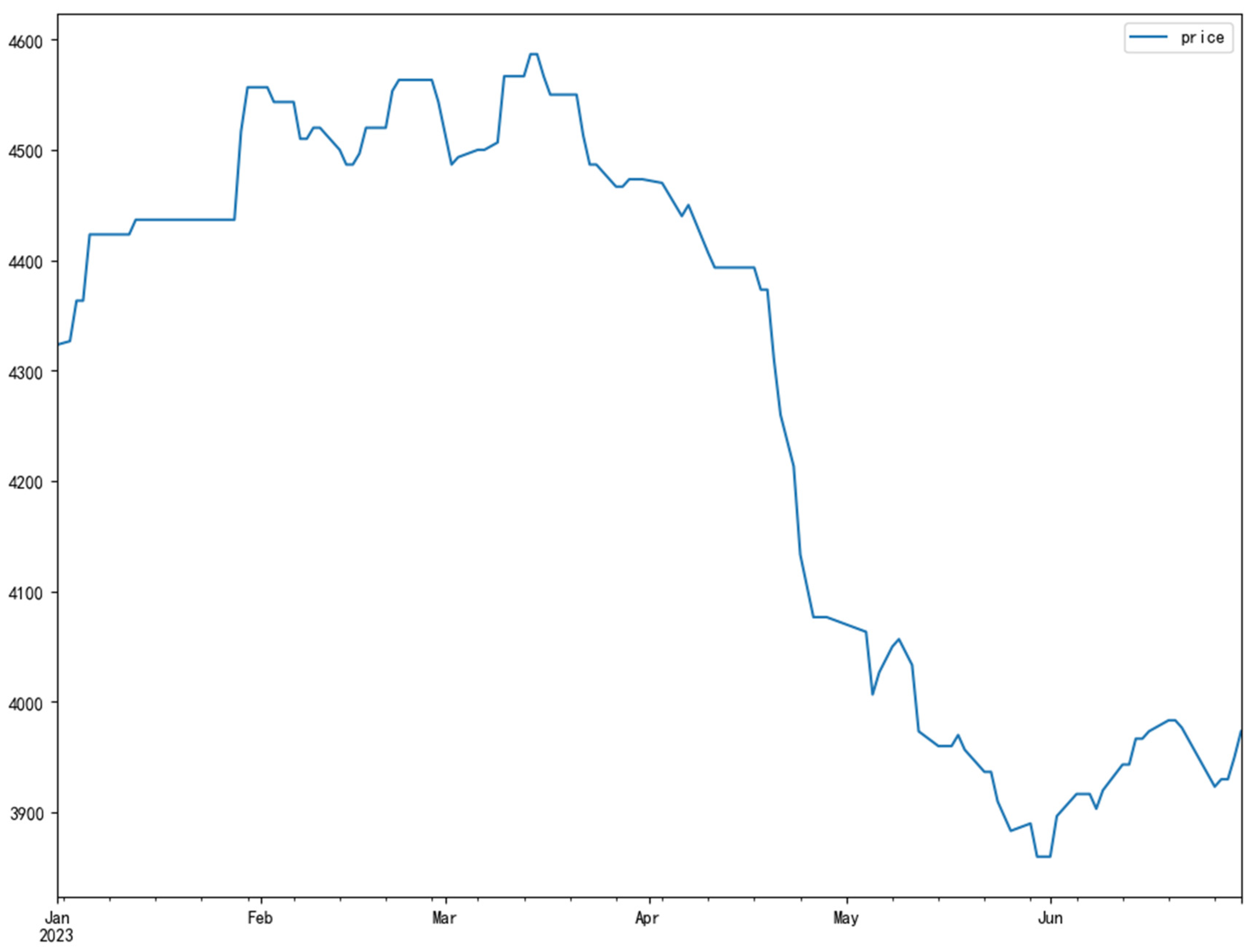
2.1.1. Price Chart
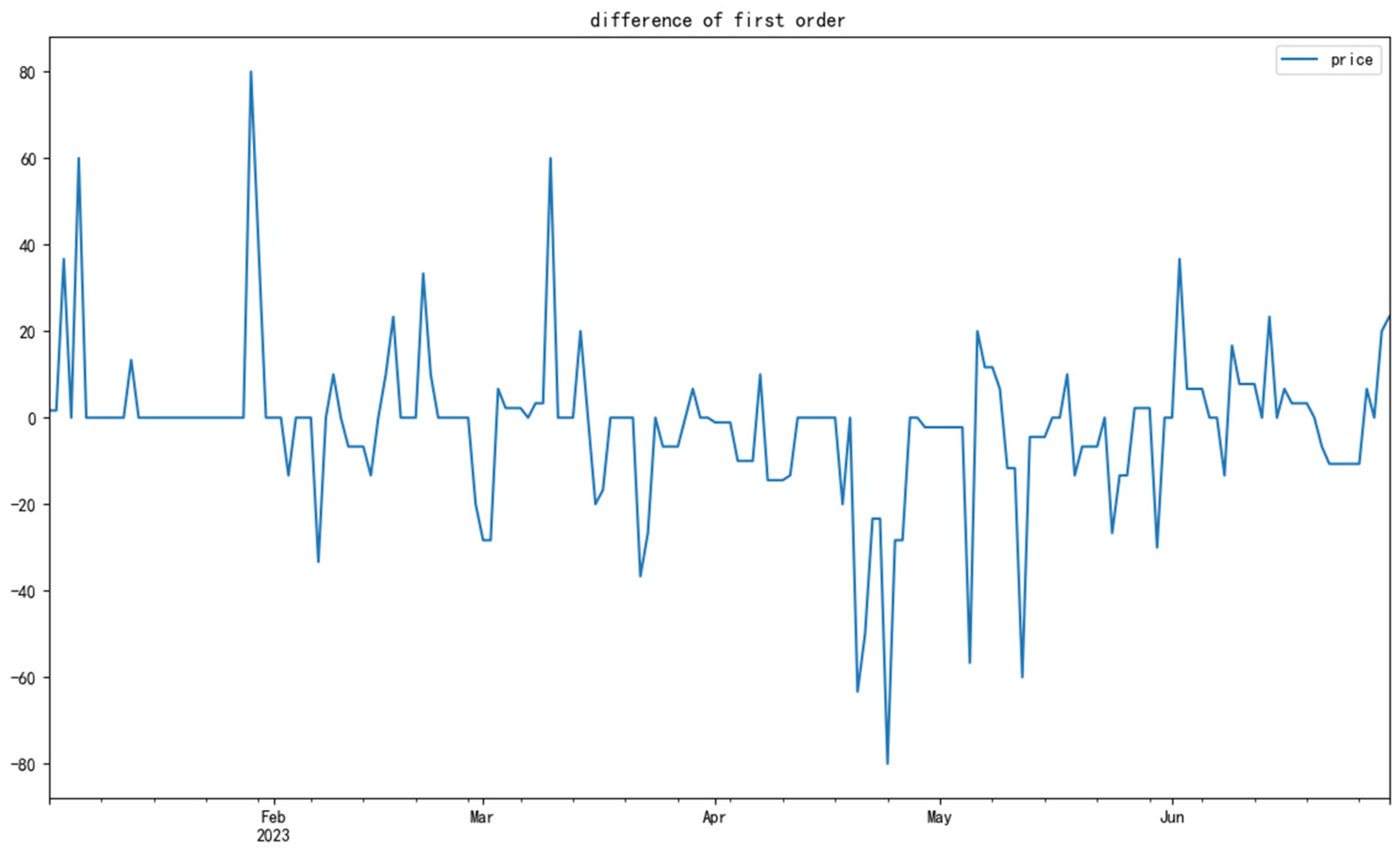
2.1.2. Stability Testing
2.1.3. Seasonal Testing
2.1.4. White Noise Testing
2.1.5. Grey Correlation and Time Series Level Ratio Detection
2.1.6. Model Selection
2.2. GM
2.3. SARIMA
2.4. Model Evaluation Indicators
3. Methodology
3.1. Survey Data
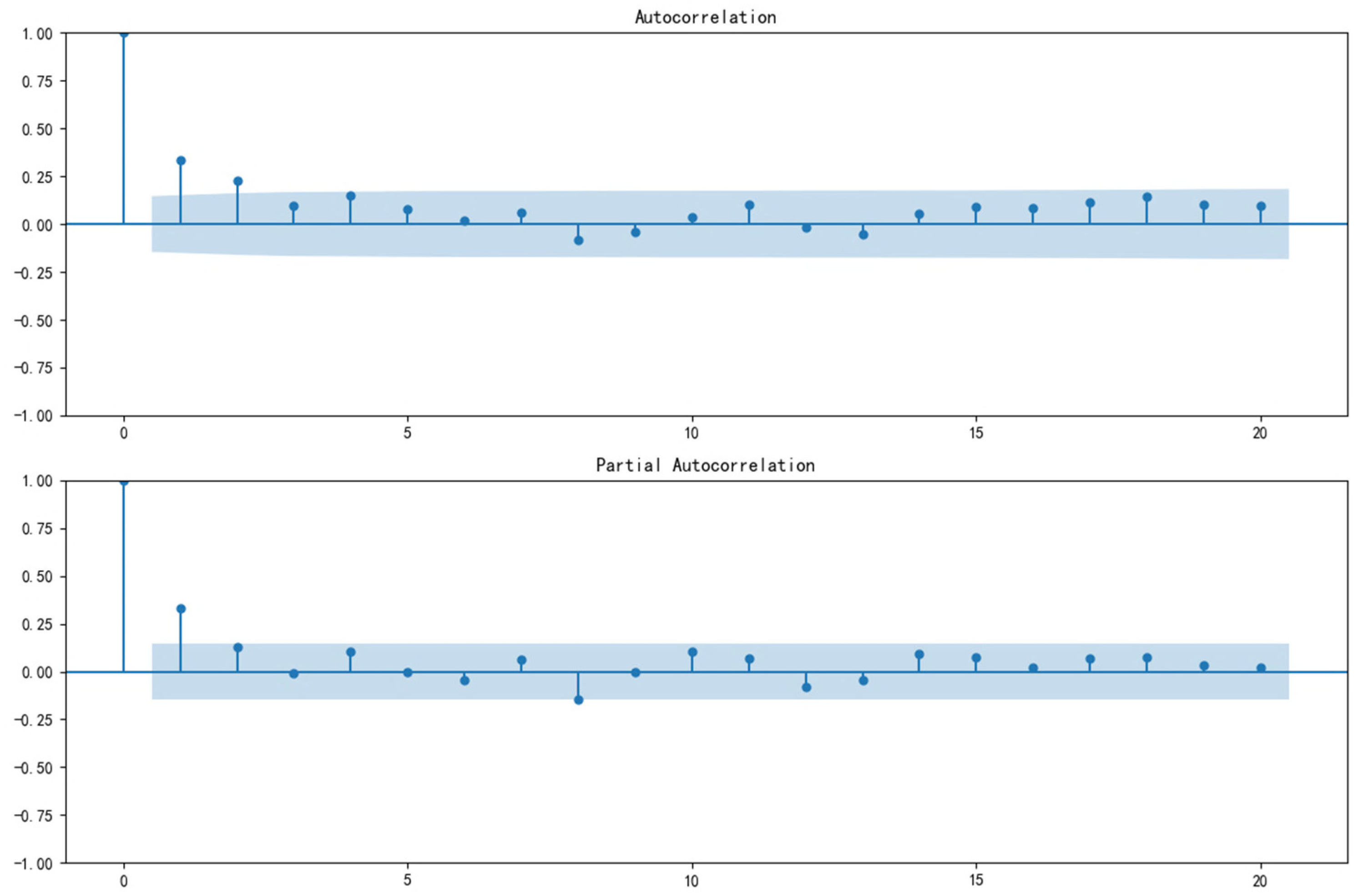
3.2. Identification and Estimation
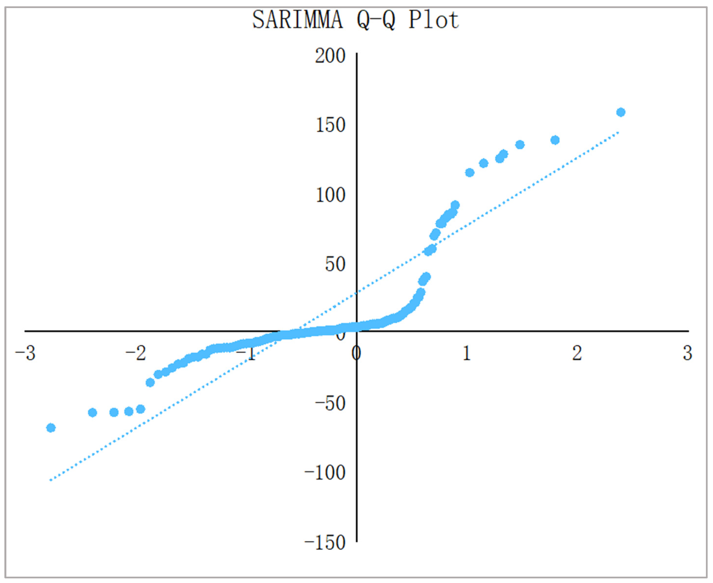
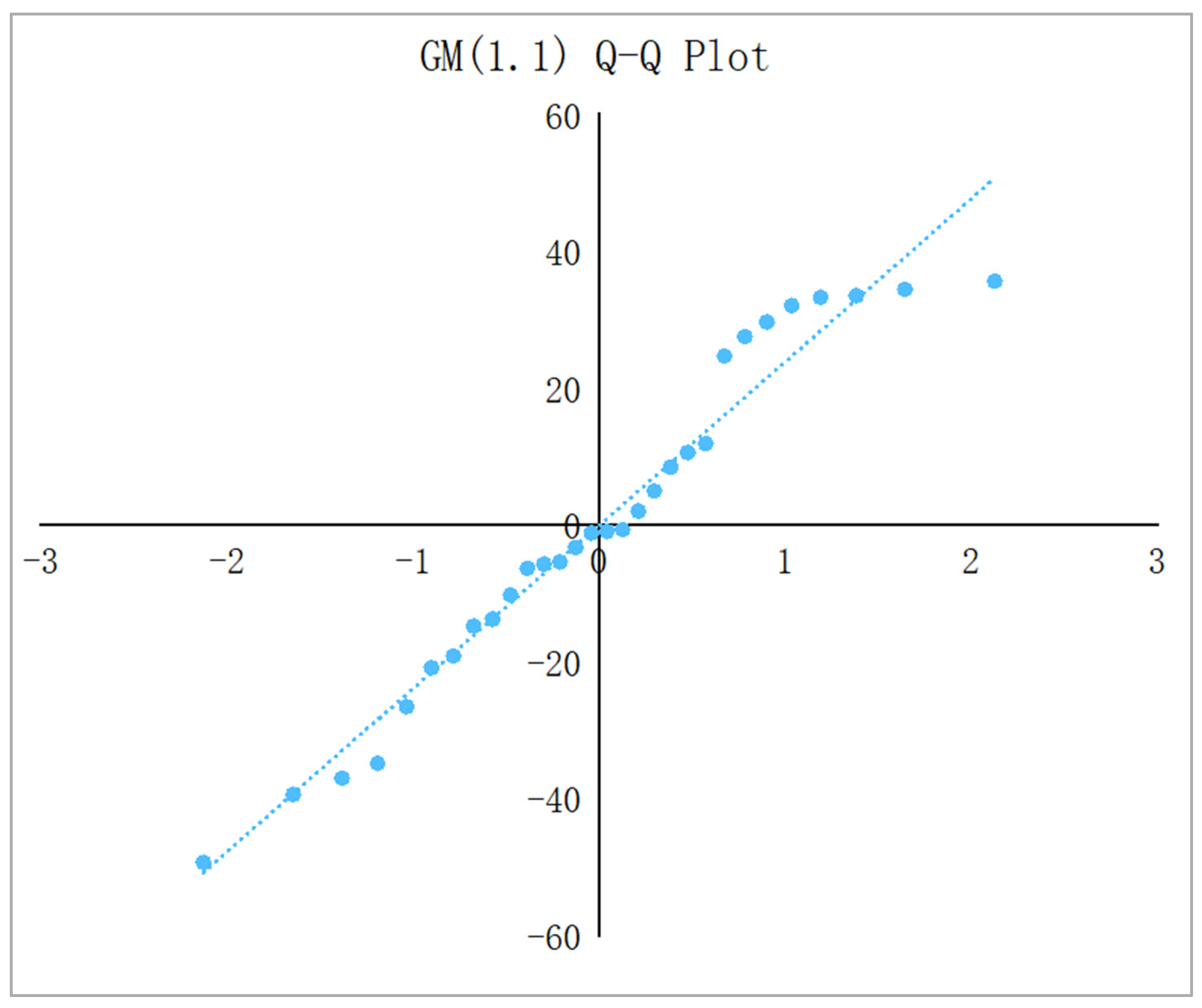
3.3. Model Validation
3.4. Combination of Models
4. Analysis and Discussion of Results
4.1. Data Series
4.2. Model Identification
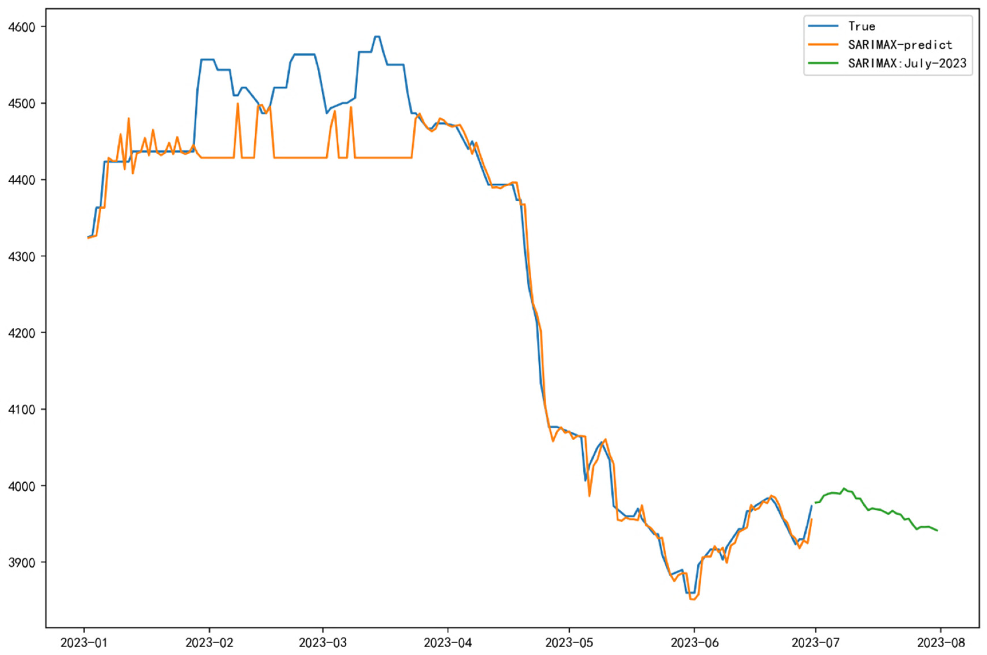
4.2.1. SARIMA
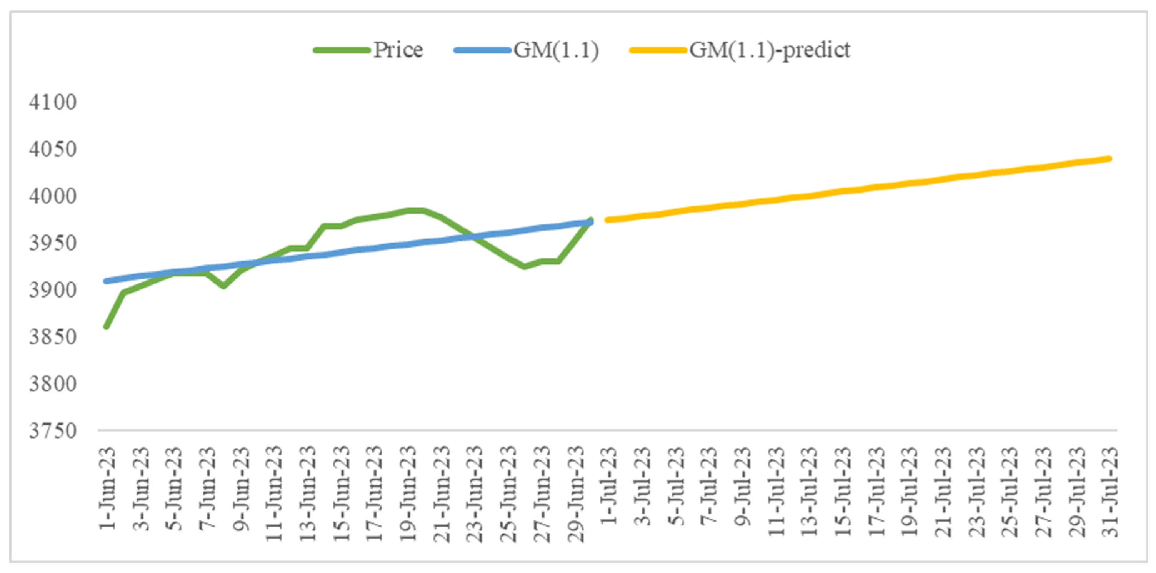
4.2.2. GM (1.1)
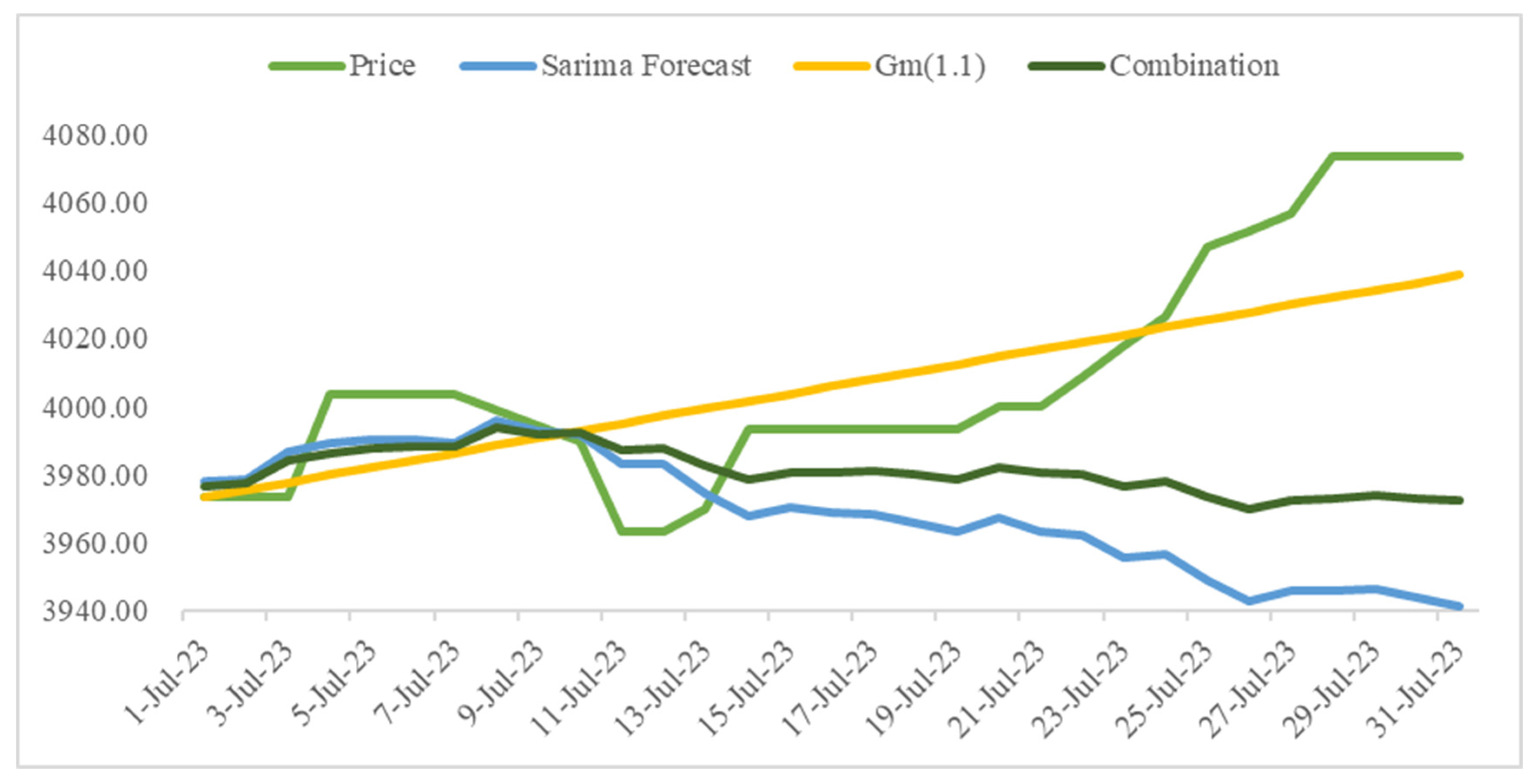
4.3. Evaluation of the Combined Model Results
5. Conclusions
Author Contributions
Funding
Data Availability Statement
Conflicts of Interest
Appendix A
| Jan | Feb | Mar | Apr | May | Jun | Jul | |
| 1 | 4091.00 | 4084.00 | 4216.00 | 4122.00 | 3570.50 | 3446.00 | 3593.67 |
| 2 | 4077.00 | 4042.00 | 4225.00 | 4083.00 | 3566.33 | 3491.00 | 3602.33 |
| 3 | 4063.00 | 4055.00 | 4272.00 | 4044.00 | 3562.17 | 3499.67 | 3611.00 |
| 4 | 4027.00 | 4053.00 | 4251.33 | 4018.00 | 3558.00 | 3508.33 | 3623.00 |
| 5 | 4017.00 | 4051.00 | 4230.67 | 3999.50 | 3542.00 | 3517.00 | 3608.00 |
| 6 | 4107.00 | 4049.00 | 4210.00 | 3981.00 | 3566.67 | 3525.00 | 3606.00 |
| 7 | 4102.33 | 4018.00 | 4033.00 | 4033.00 | 3591.33 | 3496.00 | 3511.00 |
| 8 | 4097.67 | 4055.00 | 4249.00 | 4014.67 | 3616.00 | 3503.00 | 3518.00 |
| 9 | 4093.00 | 4085.00 | 4313.00 | 3996.33 | 3588.00 | 3558.00 | 3525.00 |
| 10 | 4124.00 | 4074.00 | 4314.00 | 3978.00 | 3537.00 | 3544.67 | 3532.00 |
| 11 | 4164.00 | 4047.00 | 4333.00 | 3984.00 | 3480.00 | 3531.33 | 3550.00 |
| 12 | 4136.00 | 4020.00 | 4352.00 | 3956.00 | 3415.00 | 3518.00 | 3586.00 |
| 13 | 4173.00 | 3993.00 | 4371.00 | 3933.00 | 3437.33 | 3588.00 | 3588.00 |
| 14 | 4146.33 | 4027.00 | 4373.00 | 3945.00 | 3459.67 | 3594.00 | 3630.00 |
| 15 | 4119.67 | 4066.00 | 4332.00 | 3950.00 | 3482.00 | 3611.00 | 3612.00 |
| 16 | 4093.00 | 4146.00 | 4205.00 | 3955.00 | 3524.00 | 3654.00 | 3594.00 |
| 17 | 4119.00 | 4167.00 | 4262.00 | 3960.00 | 3595.00 | 3643.00 | 3576.00 |
| 18 | 4165.00 | 4172.67 | 4239.33 | 3971.00 | 3574.00 | 3632.00 | 3627.00 |
| 19 | 4196.00 | 4178.33 | 4216.67 | 3949.00 | 3535.00 | 3621.00 | 3623.00 |
| 20 | 4179.00 | 4184.00 | 4194.00 | 3928.00 | 3508.00 | 3595.00 | 3678.00 |
| 21 | 4181.20 | 4254.00 | 4156.00 | 3828.00 | 3481.00 | 3555.00 | 3698.00 |
| 22 | 4183.40 | 4237.00 | 4153.00 | 3794.67 | 3454.00 | 3538.00 | 3694.00 |
| 23 | 4185.60 | 4228.00 | 4070.00 | 3761.33 | 3478.00 | 3538.00 | 3690.00 |
| 24 | 4187.80 | 4224.00 | 4107.00 | 3728.00 | 3390.00 | 3538.00 | 3686.00 |
| 25 | 4190.00 | 4213.00 | 4106.33 | 3700.00 | 3352.00 | 3538.00 | 3742.00 |
| 26 | 4192.20 | 4202.00 | 4105.67 | 3698.00 | 3399.00 | 3538.00 | 3746.00 |
| 27 | 4194.40 | 4191.00 | 4105.00 | 3679.00 | 3406.33 | 3590.00 | 3782.00 |
| 28 | 4196.60 | 4174.00 | 4136.00 | 3583.00 | 3413.67 | 3594.00 | 3786.00 |
| 29 | 4198.80 | 4151.00 | 3578.83 | 3421.00 | 3582.00 | 3776.33 | |
| 30 | 4201.00 | 4167.00 | 3574.67 | 3372.00 | 3585.00 | 3766.67 | |
| 31 | 4143.00 | 4161.00 | 3374.00 | 3757.00 |
References
- Hwang, S.; Park, M.; Lee, H.-S.; Kim, H. Automated Time-Series Cost Forecasting System for Construction Materials. J. Constr. Eng. Manag. 2012, 138, 1259–1269. [Google Scholar] [CrossRef]
- Smith, J.P.; Miller, K.; Christofferson, J.; Hutchings, M. Best Practices for Dealing with Price Volatility in Utah’s Residential Construction Market. Int. J. Constr. Educ. Res. 2011, 7, 210–225. [Google Scholar] [CrossRef]
- Li, J.F.; Shen, Y.; Xu, L.J.; Suo, Y. Material Price Risks Impact on Project Costs Research. Adv. Mater. Res. 2011, 243–249, 6344–6347. [Google Scholar] [CrossRef]
- Vivek, A.; Hanumantha Rao, C.H. Identification and Analysing of Risk Factors Affecting Cost of Construction Projects. Mater. Today Proc. 2022, 60, 1696–1701. [Google Scholar] [CrossRef]
- Yang, G.; Huang, G.; Gao, H. Research on the Strategy of Construction Material Procurement When the Price Fluctuation Is Considered. In Proceedings of the 2010 International Conference on Management and Service Science, Wuhan, China, 24–26 August 2010; IEEE: New York, NY, USA, 2010; pp. 1–4. [Google Scholar]
- Al-Hammad, I.A. Treatment of Reinforcing Steel Bars Prices Fluctuations. J. King Saud Univ.—Eng. Sci. 2006, 19, 43–62. [Google Scholar] [CrossRef]
- Lin, Y.-H.; Lee, P.-C. Novel High-Precision Grey Forecasting Model. Autom. Constr. 2007, 16, 771–777. [Google Scholar] [CrossRef]
- Zhang, D.; Ning, X.; Liu, X.; Han, Y. Nonlinear Time Series Forecasting with Dynamic RBF Neural Networks. In Proceedings of the 2008 7th World Congress on Intelligent Control and Automation, Chongqing, China, 25–27 June 2008; IEEE: New York, NY, USA, 2008; pp. 6988–6993. [Google Scholar]
- Kapl, M.; Müller, W.G. Prediction of Steel Prices: A Comparison between a Conventional Regression Model and MSSA. Stat. Interface 2010, 3, 369–375. [Google Scholar] [CrossRef]
- Wu, B.; Zhu, Q. Week-Ahead Price Forecasting for Steel Market Based on RBF NN and ASW. In Proceedings of the 2012 IEEE International Conference on Computer Science and Automation Engineering, Beijing, China, 22–24 June 2012; IEEE: New York, NY, USA, 2012; pp. 729–732. [Google Scholar]
- Yin, Y.; Wu, B.; Zhu, Q. Compare with Three Models for Price Forecasting on Steel Market. In Proceedings of the 2012 International Conference on Computer Science and Service System, Nanjing, China, 11–13 August 2012; IEEE: New York, NY, USA, 2012; pp. 1844–1847. [Google Scholar]
- Feng, Z.; Ren, Q. Forecasting Model with Dynamical Combined Residual Error Correction. Syst. Eng.–Theory Pract. 2017, 37, 1884–1991. [Google Scholar]
- Wang, Q.K.; Mei, T.T.; Guo, Z.; Kong, L.W. Building Material Price Forecasting Based on Multi-Method in China. In Proceedings of the 2018 IEEE International Conference on Industrial Engineering and Engineering Management (IEEM), Bangkok, Thailand, 16–19 December 2018; IEEE: New York, NY, USA, 2018; pp. 1826–1830. [Google Scholar]
- Faghih, S.A.M.; Kashani, H. Forecasting Construction Material Prices Using Vector Error Correction Model. J. Constr. Eng. Manag. 2018, 144, 04018075. [Google Scholar] [CrossRef]
- Shiha, A.; Dorra, E.M.; Nassar, K. Neural Networks Model for Prediction of Construction Material Prices in Egypt Using Macroeconomic Indicators. J. Constr. Eng. Manag. 2020, 146, 04020010. [Google Scholar] [CrossRef]
- Mir, M.; Kabir, H.M.D.; Nasirzadeh, F.; Khosravi, A. Neural Network-Based Interval Forecasting of Construction Material Prices. J. Build. Eng. 2021, 39, 102288. [Google Scholar] [CrossRef]
- Xu, X.; Zhang, Y. Price Forecasts of Ten Steel Products Using Gaussian Process Regressions. Eng. Appl. Artif. Intell. 2023, 126, 106870. [Google Scholar] [CrossRef]
- Zhang, Q. Research on the Improved Combinatorial Prediction Model of Steel Price Based on Time Series. Teh. Vjesn. 2023, 30, 2018–2025. [Google Scholar] [CrossRef]
- Mi, J.; Xie, X.; Luo, Y.; Zhang, Q.; Wang, J. Research on Rebar Futures Price Forecast Based on VMD–EEMD–LSTM Model. In Advances in Transdisciplinary Engineering; Chen, C.-H., Scapellato, A., Barbiero, A., Korzun, D.G., Eds.; IOS Press: Amsterdam, The Netherlands, 2023; ISBN 978-1-64368-458-1. [Google Scholar]
- Liu, S. A Study of Short-Term Forecasting of Raw Material Prices Using a Combined LSTM-ARIMA Model. In Proceedings of the International Conference on Cloud Computing, Performance Computing, and Deep Learning (CCPCDL 2023), Huzhou, China, 25 May 2023; Subramaniam, K., Saxena, S., Eds.; SPIE: Bellingham, WA, USA, 2023; p. 46. [Google Scholar]
- Sangkhiew, N.; Watanasungsuit, A.; Inthawongse, C.; Jomthong, P.; Saicharoen, K.; Pornsing, C. Adaptive Holt-Winters Forecasting Method Based on Artificial Intelligence Techniques. In Proceedings of the 2023 17th International Conference on Ubiquitous Information Management and Communication (IMCOM), Seoul, Republic of Korea, 3 January 2023; IEEE: New York, NY, USA, 2023; pp. 1–5. [Google Scholar]
- Ju-Long, D. Control Problems of Grey Systems. Syst. Control Lett. 1982, 1, 288–294. [Google Scholar] [CrossRef]
- Vallée, R. Grey Information: Theory and Practical Applications. Kybernetes 2008, 37, 189. [Google Scholar] [CrossRef]
- Bai, C.; Sarkis, J. Integrating Sustainability into Supplier Selection with Grey System and Rough Set Methodologies. Int. J. Prod. Econ. 2010, 124, 252–264. [Google Scholar] [CrossRef]
- Heng, Z. Analysis of Infrared Images Based on Grey System and Neural Network. Kybernetes 2010, 39, 1366–1375. [Google Scholar] [CrossRef]
- Olson, D.L.; Wu, D. Simulation of Fuzzy Multiattribute Models for Grey Relationships. Eur. J. Oper. Res. 2006, 175, 111–120. [Google Scholar] [CrossRef]
- Wang, R.; Yao, L.; Li, Y. A Hybrid Forecasting Method for Day-Ahead Electricity Price Based on GM(1,1) and ARMA. In Proceedings of the 2009 IEEE International Conference on Grey Systems and Intelligent Services (GSIS 2009), Nanjing, China, 10–12 November 2009; IEEE: New York, NY, USA, 2009; pp. 577–581. [Google Scholar]
- Wei, G.-W. Grey Relational Analysis Method for 2-Tuple Linguistic Multiple Attribute Group Decision Making with Incomplete Weight Information. Expert Syst. Appl. 2011, 38, 4824–4828. [Google Scholar] [CrossRef]
- Liu, S.; Forrest, J.Y.L. Grey Systems: Theory and Applications. Grey Syst. Theory Appl. 2011, 1, 274–275. [Google Scholar] [CrossRef]
- Tan, Y.; Xu, H.; Hui, E.C.M. Forecasting Property Price Indices in Hong Kong Based on Grey Models. Int. J. Strateg. Prop. Manag. 2017, 21, 256–272. [Google Scholar] [CrossRef]
- Wang, C.; Sun, Z. Monthly Pork Price Forecasting Method Based on Census X12-GM(1,1) Combination Model. PLoS ONE 2021, 16, e0251436. [Google Scholar] [CrossRef] [PubMed]
- Yang, J. Electricity Price Forecast Based on Metabolic GM(1,1) Model under Wind Power Development Prospect. In Proceedings of the 2022 IEEE 9th International Conference on Power Electronics Systems and Applications (PESA), Hong Kong, 20 September 2022; IEEE: New York, NY, USA, 2022; pp. 1–7. [Google Scholar]
- Yang, W.; Wu, X.; Zhang, E.; Zhu, G. Application of GM (1,N)-Markov Model in Shanghai Composite Index Prediction. In The 19th International Conference on Industrial Engineering and Engineering Management; Qi, E., Shen, J., Dou, R., Eds.; Springer: Berlin/Heidelberg, Germany, 2013; pp. 625–635. ISBN 978-3-642-37269-8. [Google Scholar]
- Yao, T.; Wang, Z. Crude Oil Price Prediction Based on LSTM Network and GM (1,1) Model. Grey Syst.-Theory Appl. 2021, 11, 80–94. [Google Scholar] [CrossRef]
- Si, G.Z. Stock Prediction with Grey Neural Network Model. Comput. Simul. 2012, 29, 382–385,415. [Google Scholar]
- Çevrimli, M.B.; Arikan, M.S.; TekïNdal, M.A. Honey Price Estimation for the Future in Turkey; Example of 2019–2020. Ank. Üniv. Vet. Fak. Derg. 2020, 67, 143–152. [Google Scholar] [CrossRef]
- Daryl; Winata, A.; Kumara, S.; Suhartono, D. Predicting Stock Market Prices Using Time Series SARIMA. In Proceedings of the 2021 1st International Conference on Computer Science and Artificial Intelligence (ICCSAI), Jakarta, Indonesia, 28 October 2021; IEEE: New York, NY, USA, 2021; pp. 92–99. [Google Scholar]
- Preetha, K.G.; Babu, K.R.R.; Sangeetha, U.; Thomas, R.S.; Saigopika; Walter, S.; Thomas, S. Price Forecasting on a Large Scale Data Set Using Time Series and Neural Network Models. KSII Trans. Internet Inf. Syst. 2022, 16, 3923–3942. [Google Scholar] [CrossRef]
- Luo, C.S.; Zhou, L.Y.; Wei, Q.F. Application of SARIMA Model in Cucumber Price Forecast. Appl. Mech. Mater. 2013, 373–375, 1686–1690. [Google Scholar] [CrossRef]
- Theerthagiri, P.; Ruby, A.U. Seasonal Learning Based ARIMA Algorithm for Prediction of Brent Oil Price Trends. Multimed. Tools Appl. 2023, 82, 24485–24504. [Google Scholar] [CrossRef]
- Yuan, H.; Zhang, D.; Xu, W.; Wang, M.; Dong, W. Forecasting the CPI Using a Hybrid Sarima and Neural Network Model with Web News Articles. In Proceedings of the 2013 Sixth International Conference on Business Intelligence and Financial Engineering, Hangzhou, China, 14–16 November 2013; IEEE: New York, NY, USA, 2013; pp. 84–88. [Google Scholar]
- Zhang, J.; Tan, Z.; Wei, Y. An Adaptive Hybrid Model for Short Term Electricity Price Forecasting. Appl. Energy 2020, 258, 114087. [Google Scholar] [CrossRef]
- Paraschiv, D.M.; Balasoiu, N.; Ben-Amor, S.; Bag, R.C. Hybridising Neurofuzzy Model the Seasonal Autoregressive Models for Electricity Price Forecasting on Germanys Spot Market. Amfiteatru Econ. 2023, 25, 463. [Google Scholar] [CrossRef]
- Cheng, J.; Tiwari, S.; Khaled, D.; Mahendru, M.; Shahzad, U. Forecasting Bitcoin Prices Using Artificial Intelligence: Combination of ML, SARIMA, and Facebook Prophet Models. Technol. Forecast. Soc. Chang. 2024, 198, 122938. [Google Scholar] [CrossRef]
- Martins, V.L.M.; Werner, L. Forecast Combination in Industrial Series: A Comparison between Individual Forecasts and Its Combinations with and without Correlated Errors. Expert Syst. Appl. 2012, 39, 11479–11486. [Google Scholar] [CrossRef]
- Kumar, D.S.; Thiruvarangan, B.C.; Vishnu, A.; Devi, A.S.; Kavitha, D. Analysis and Prediction of Stock Price Using Hybridization of SARIMA and XGBoost. In Proceedings of the 2022 International Conference on Communication, Computing and Internet of Things (IC3IoT), Chennai, India, 10 March 2022; IEEE: New York, NY, USA, 2022; pp. 1–4. [Google Scholar]
- Kumar, V.; Singh, N.; Singh, D.K.; Mohanty, S.R. Short-Term Electricity Price Forecasting Using Hybrid SARIMA and GJR-GARCH Model. In Networking Communication and Data Knowledge Engineering; Perez, G.M., Mishra, K.K., Tiwari, S., Trivedi, M.C., Eds.; Lecture Notes on Data Engineering and Communications Technologies; Springer: Singapore, 2018; Volume 3, pp. 299–310. ISBN 978-981-10-4584-4. [Google Scholar]
- Xiang, Y. Using ARIMA-GARCH Model to Analyze Fluctuation Law of International Oil Price. Math. Probl. Eng. 2022, 2022, 3936414. [Google Scholar] [CrossRef]
- Zhang, J.; Liu, H.; Bai, W.; Li, X. A Hybrid Approach of Wavelet Transform, ARIMA and LSTM Model for the Share Price Index Futures Forecasting. N. Am. J. Econ. Financ. 2024, 69, 102022. [Google Scholar] [CrossRef]
- Guo, Z.; Wu, B.; Ma, X.; Chen, J. Forecasting Gas Emission Concentration Using Wavelet Decomposition and GM-ARIMA Model. J. Mines Met. Fuels 2016, 64, 612. [Google Scholar]


| Jan–Feb | Feb–Mar | Mar–Apr | Apr–May | May–Jun | |
|---|---|---|---|---|---|
| 0.675 | 0.904 | 0.625 | 0.821 | 0.598 |
| Jan | Feb | Mar | Apr | May | Jun | |
|---|---|---|---|---|---|---|
| 1.000 | 1.007 | 1.008 | 1.019 | 1.015 | 1.003 | |
| 0.982 | 0.993 | 0.987 | 0.998 | 0.995 | 0.991 |
| n = 28 | n = 30 | n = 31 | |
|---|---|---|---|
| 0.929 | 0.933 | 0.936 | |
| 1.069 | 1.064 | 1.062 |
| Min | Max | |
|---|---|---|
| ps | 0 | 4 |
| qs | 0 | 4 |
| Ps | 0 | 3 |
| Qs | 0 | 3 |
| D | 0 | 2 |
| RMSE | MAE | MAPE |
|---|---|---|
| 59.43 | 36.28 | 0.83% |
| RMSE | MAE | MAPE |
|---|---|---|
| 23.82 | 19.27 | 0.49% |
| Day | Price | SARIMA | GM (1.1) | Combinational Model |
|---|---|---|---|---|
| 1 Jul 23 | 3973.33 | 3977.86 | 3973.44 | 3976.46 |
| 2 Jul 23 | 3973.33 | 3978.62 | 3975.59 | 3977.66 |
| 3 Jul 23 | 3973.33 | 3986.86 | 3977.75 | 3983.98 |
| 4 Jul 23 | 4003.33 | 3989.11 | 3979.91 | 3986.19 |
| 5 Jul 23 | 4003.33 | 3990.54 | 3982.07 | 3987.86 |
| 6 Jul 23 | 4003.33 | 3990.27 | 3984.23 | 3988.36 |
| 7 Jul 23 | 4003.33 | 3989.30 | 3986.39 | 3988.38 |
| 8 Jul 23 | 3998.89 | 3996.15 | 3988.55 | 3993.74 |
| 9 Jul 23 | 3994.44 | 3992.73 | 3990.71 | 3992.09 |
| 10 Jul 23 | 3990.00 | 3992.03 | 3992.88 | 3992.30 |
| 11 Jul 23 | 3963.33 | 3983.30 | 3995.05 | 3987.02 |
| 12 Jul 23 | 3963.33 | 3983.12 | 3997.21 | 3987.58 |
| 13 Jul 23 | 3970.00 | 3974.75 | 3999.38 | 3982.55 |
| 14 Jul 23 | 3993.33 | 3967.93 | 4001.55 | 3978.58 |
| 15 Jul 23 | 3993.33 | 3970.28 | 4003.72 | 3980.87 |
| 16 Jul 23 | 3993.33 | 3969.11 | 4005.89 | 3980.76 |
| 17 Jul 23 | 3993.33 | 3968.44 | 4008.07 | 3980.99 |
| 18 Jul 23 | 3993.33 | 3965.84 | 4010.24 | 3979.90 |
| 19 Jul 23 | 3993.33 | 3963.15 | 4012.42 | 3978.75 |
| 20 Jul 23 | 4000.00 | 3967.17 | 4014.59 | 3982.19 |
| 21 Jul 23 | 4000.00 | 3963.54 | 4016.77 | 3980.40 |
| 22 Jul 23 | 4008.89 | 3962.31 | 4018.95 | 3980.25 |
| 23 Jul 23 | 4017.78 | 3955.65 | 4021.13 | 3976.39 |
| 24 Jul 23 | 4026.67 | 3956.91 | 4023.31 | 3977.94 |
| 25 Jul 23 | 4046.67 | 3949.21 | 4025.49 | 3973.37 |
| 26 Jul 23 | 4051.67 | 3943.02 | 4027.68 | 3969.84 |
| 27 Jul 23 | 4056.67 | 3946.09 | 4029.86 | 3972.62 |
| 28 Jul 23 | 4073.33 | 3945.99 | 4032.05 | 3973.25 |
| 29 Jul 23 | 4073.33 | 3946.32 | 4034.23 | 3974.16 |
| 30 Jul 23 | 4073.33 | 3943.97 | 4036.42 | 3973.25 |
| 31 Jul 23 | 4073.33 | 3941.51 | 4038.61 | 3972.27 |
| SARIMA | GM (1.1) | Combination Model | |
|---|---|---|---|
| RMSE | 9.90 | 13.44 | 10.77 |
| MAE | 8.39 | 10.45 | 9.04 |
| MAPE | 0.21% | 0.26% | 0.23% |
| SARIMA | GM (1.1) | Combination Model | |
|---|---|---|---|
| RMSE | 18.60 | 17.66 | 13.89 |
| MAE | 15.83 | 14.80 | 12.44 |
| MAPE | 0.40% | 0.37% | 0.31% |
| SARIMA | GM (1.1) | Combination Model | |
|---|---|---|---|
| RMSE | 61.99 | 21.39 | 46.96 |
| MAE | 43.99 | 17.85 | 33.12 |
| MAPE | 1.09% | 0.44% | 0.82% |
Disclaimer/Publisher’s Note: The statements, opinions and data contained in all publications are solely those of the individual author(s) and contributor(s) and not of MDPI and/or the editor(s). MDPI and/or the editor(s) disclaim responsibility for any injury to people or property resulting from any ideas, methods, instructions or products referred to in the content. |
© 2024 by the authors. Licensee MDPI, Basel, Switzerland. This article is an open access article distributed under the terms and conditions of the Creative Commons Attribution (CC BY) license (https://creativecommons.org/licenses/by/4.0/).
Share and Cite
Dai, X.; Gao, P.; Ma, S. Cost Forecasting for Building Rebar under Uncertainty Conditions: Methodology and Practice. Buildings 2024, 14, 1900. https://doi.org/10.3390/buildings14071900
Dai X, Gao P, Ma S. Cost Forecasting for Building Rebar under Uncertainty Conditions: Methodology and Practice. Buildings. 2024; 14(7):1900. https://doi.org/10.3390/buildings14071900
Chicago/Turabian StyleDai, Xiaomin, Peng Gao, and Shengqiang Ma. 2024. "Cost Forecasting for Building Rebar under Uncertainty Conditions: Methodology and Practice" Buildings 14, no. 7: 1900. https://doi.org/10.3390/buildings14071900