Abstract
The performance gap caused by occupant behaviour (OB) is one of the main challenges to the accuracy of building performance simulations (BPS) models. Calibration of BPS models has shown great improvements in tertiary and single residential buildings. Nevertheless, the calibration in collective residential buildings is still uncertain. This study aims to identify the opportunities and barriers to the calibration of collective residential building BPS models for the analysis of heating energy consumption. For this, the research calibrates a real case study of a social rental housing building located in northern Spain. The method involves the adjustment of input data based on OB clusters, developed by monitorization and survey data and the statistical comparison of the results of normative models, calibrated models and real data. The results show an average improvement of 67% in hourly indoor temperature and 16% in hourly heating energy consumption in calibrated models, but still with a considerable performance gap. The main barriers to a higher accuracy are the wide diversity and lack of uniformity of OB patterns, uncertainty of parameters, and use of auxiliary heating systems. However, deeper monitorization and survey campaigns with the use of OB clusters can be a promising opportunity.
1. Introduction
The use of building energy modelling (BEM) has become increasingly common in the field of architecture in recent years. It is widely applied in building performance simulation (BPS) or building energy simulation (BES) during the processes of design, management (operation), and renovation of buildings. The accurate energetic analysis of buildings is essential for an evaluation in pursuit of the reduction of environmental impact of buildings required by the European Union (EU) energy policy as put forward in the last Energy Performance of Buildings Directive (EPBD) (Directive (EU) 2024/1275 [1,2]). This would include accurate data for energy management, analysis of energy renovation strategies, and the assessment of decarbonisation progress. BPS refers to a mathematical model that allows for a detailed calculation of a building’s energy performance and the thermal comfort of its occupants. This model considers various parameters such as climate data, building geometry, internal gains, heating and cooling systems, building use, and occupancy, among others [3].
There are several tools available for building energy simulation, including DOE-2 [4], EnergyPlus [5], TRNSYS [6], and ESP-r [7]. Among these tools, EnergyPlus is most commonly employed, as indicated by the review conducted by Chong et al. [3]. These programs define simulation models for different purposes, such as building design, heating and cooling system design and management, analysis of refurbishment proposals, optimisation of building performance, and analysis of building energy efficiency and equipment.
However, previous research has shown that there is a performance gap between simulated and real building models [8,9]. This performance gap can be attributed to standard building models, generic climate data, and discrepancies between the design and the actual building. Differences between simulated and real building performance models can also affect interventions’ environmental impact, energy efficiency, and economic and environmental viability [10].
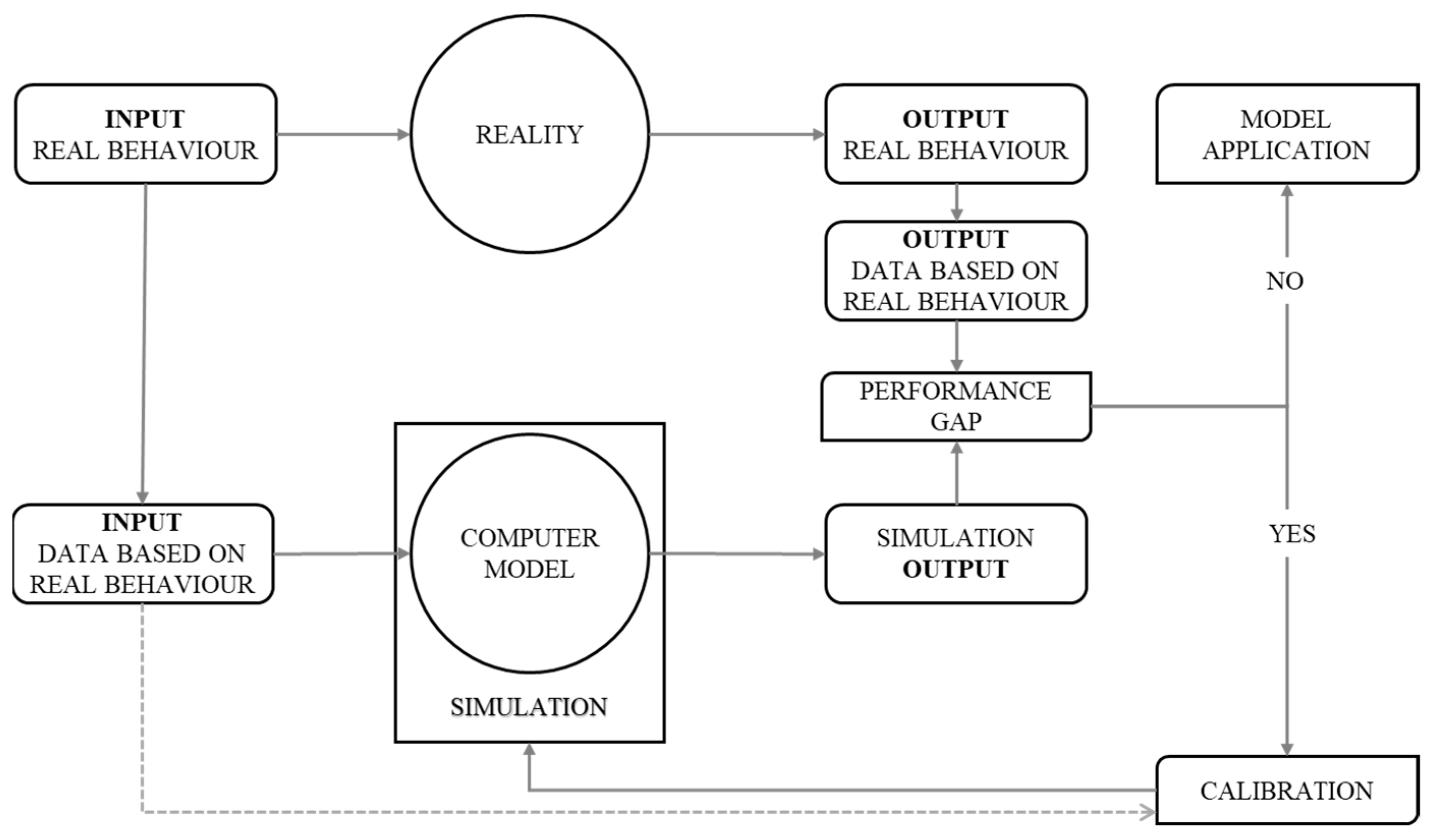
The use of real data can help reduce this performance gap through the calibration of simulation models [11]. A simulation model represents the actual building performance, and the goal of calibration is to make the model as accurate as possible in reflecting the real performance. In other words, the parameters used in calibration are adjusted to align the simulation results with the actual performance [3] (see Figure 1). Ultimately, the objective of calibration is to minimise discrepancies between measured and simulated data [12].

Figure 1.
Illustration of the calibration process based on [3].
According to ASHRAE guidelines 14-2014 [13], calibration reduces the uncertainty of a model by comparing it with real data measured under identical conditions. Calibration helps identify the parameters that require adjustment and establishes an acceptable level of uncertainty. Calibration aims to minimise discrepancies between simulated and real building performance data.
Calibration, validation, and verification of simulation models are essential for assessing the consistency between the prediction model and real-world observations [3]. Calibration involves adjusting the numerical or physical parameters of the model to improve its agreement with real data. Validation helps determine the extent to which the simulated model accurately represents the actual building performance based on the initial model target. Verification ensures that the model implementation accurately reflects the developer’s conceptual description and solution.
Coakley et al. [12] presented a comprehensive review of current model development and calibration approaches, emphasising uncertainty’s significance in the calibration process. They classified calibration approaches as either manual or automatic. Manual approaches depend on the researcher’s intervention to refine the model, whereas automatic approaches adjust the input parameters using computer processes that are not user-driven.
The literature review by Chong et al. [3] compiled the most commonly used inputs in previous research, emphasising using actual weather data such as dry bulb temperature, solar radiation, relative humidity, wind speed, and direction. Previous studies have also demonstrated the significance of weather files, indicating that the annual building energy consumption and monthly building loads can differ by approximately ±7% and ±40%, respectively, based on the provided weather data [14]. The review also identified several studies incorporating indoor environment data as model inputs to achieve a more specific calibration of indoor environments.
Regarding outputs, Chong et al. [3] exposed that automatic calibrations typically focus on parameters related to the building envelope, infiltration rate, and indoor gains. On the other hand, manual approaches tend to calibrate parameters associated with the building envelope and human behaviour, including occupancy, facility usage, lighting, and HVAC.
According to ASHRAE Guideline 14-2002 [15] and 14-2014 [13], uncertainty analysis refers to “the process of determining the level of confidence in the true value when using measurement procedures and/or calculations”. The calibrated model is assessed using various metrics, including mean bias error (MBE), normalized mean bias error (NMBE), root mean square error (RMSE), coefficient of variation of root mean square error (CV(RMSE)), and coefficient of determination (R2) [16].
The validation of a BPS model primarily relies on adherence to the limits established in ASHRAE Guideline 14 [15], the International Performance Measurement and Verification Protocol (IPMVP) [17], or the Federal Energy Management Program (FEMP) [18] for the CV(RMSE) and NMBE values [3].
In calibrating simulation models, the occupants’ behaviour (OB) is becoming increasingly important. Previous research has shown that occupants’ behaviour has a significant impact on the buildings’ energy performance [19,20], which in turn affects the behavioural gap [21]. Currently, occupant parameters are often simplified and standardised in terms of occupants’ presence, behaviour, and interaction with the building and its facilities [22]. However, households may have diverse behaviours and characteristics. Therefore, research now focuses on developing and studying OB models for application in BPS [23,24,25]. These models aim to incorporate the diversity of behaviours and the bidirectional interaction between occupants and their built environment [26]. Technological advancements and digitalisation have made it easier to collect real data by monitoring actual behaviour such as energy consumption, occupancy, thermostat use, and window opening, and via surveys that capture information like the number of people, comfort preferences, habits, and lifestyle.
Integrating OB models in BPS presents an opportunity to consider the diversity of occupants and their interaction with the building. Mahecha-Zambrano et al. [26] discussed key aspects of applying OB models, including interaction and adaptability, behavioural diversity, and building design.
However, as noted by Coakley et al. [12], the calibration of simulated models can pose challenges that limit their widespread use in the building and construction sector. These challenges include the absence of guidelines for model definition and a consensus standard for simulation calibration. Additionally, obtaining quality input data that accurately reflect the key factors influencing building performance is not always feasible. Furthermore, the level of manual adjustment required by users can impede the automation of the calibration process.
Moreover, while calibration has been extensively studied in previous research, the focus has primarily been on office, educational, and tertiary buildings [12]. The calibration of residential buildings has predominantly been examined through the analysis of individual dwellings [11], with less attention given to the calibration of multi-unit residential buildings.
Previous research has shown that regulation-based models may not accurately reflect actual behaviour, leading to discrepancies and performance gaps in BPS. Furthermore, calibration based on real data has predominantly focused on office buildings, where OB is more uniform, and occupants have less influence on HVAC systems. These discrepancies and calibration suggest that while using real data for calibrating residential buildings may lead to more accurate results than regulatory models, the calibration may not be as precise as in other building types.
Based on this context, this paper aims to provide evidence demonstrating the opportunities and challenges of calibrating models using monitored behavioural data versus standardised models in social housing. To achieve this objective, two questions have been proposed:
- How does the calibrated model improve upon the standardised model?
- What limitations discern the calibration of social and collective housing buildings?
2. Methodology
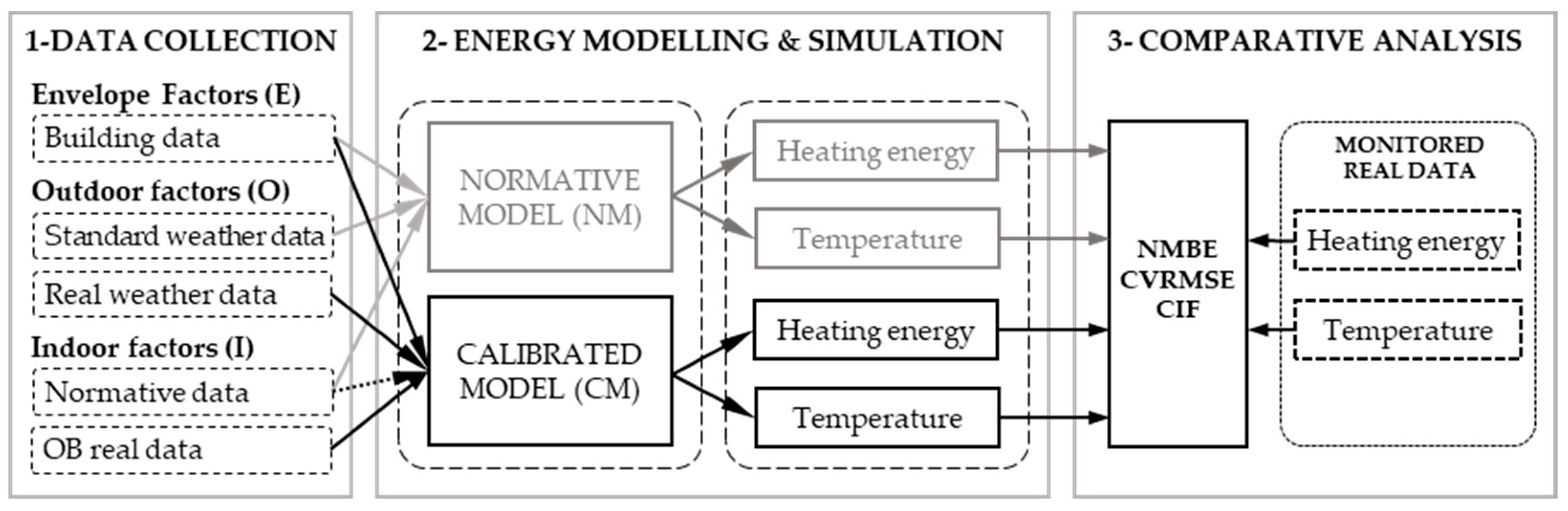
This study develops a three-stage methodology based on the comparative analysis of real monitored data with energy simulation data of the normative model (NM) and calibrated model (CM) (see Figure 2). The study analyses a real case study: a residential building located in northern Spain. On the one hand, the NM uses input parameters based on normative and standard values commonly applied in regular energy calculations of residential buildings, like the energy performance certifications (EPC); on the other hand, the CM is adjusted with input parameters based on real data obtained by different methods like monitoring, survey, and others. In terms of energy modelling and BPS, the study is exclusively focused on the analysis of the heating energy consumption of residential buildings located in climatic zones where the main energy consumption is attributed to the heating process, as the main energy consumption process of the residential stock of the EU [27]. The main targets to be analysed are the hourly heating energy consumption and the indoor dry bulb temperature in the winter season, as the object is to understand the energetic performance of the heating process. The energy modelling and BPS are done in the dynamic energy simulation tool DesignBuilder [28] with the EnergyPlus calculation engine [29], and consequently, the input data are defined according to the requirements of these tools.
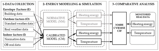
Figure 2.
Methodology algorithm based on the comparative analysis of real monitored data with BPS data of normative models (NM) and calibrated models (CM).
In summary, the first stage of the methodology carries out the data collection of the case study and normative standards to be applied. The second stage performs the energetic modelling and BPS with the collected data as inputs to obtain the output data, which will be analysed in the third stage. Finally, the third stage carries out a comparative analysis between simulated results of the NM and CM with the monitored real data, applying statistical parameters like the normalised mean bias error (NMBE), coefficient of variation of the root mean square error (CV-RMSE), and calibration improvement factor (CIF).
2.1. Data Collection
The first stage of the methodology carries out data collection to build the energy models. The data distribution follows the scheme applied by the research of E. Cuerda et al. [11], categorising the parameters of an energy model into three groups: envelope factors (E), indoor factors (I), and outdoor factors (O). The development of the NM employs building and normative data, while the CM replaces specific normative data with occupant behaviour and climate data using real measured data and carrying out the calibration process.
2.1.1. Envelope Factors (E)
The envelope factors (E) are the parameters that describe the thermal performance of the thermal envelope and architectural configuration of the studied building; the same data are used for the NM and CM. These parameters reflect the construction data, considering all the parameters that affect the energetic behaviour, such as thermal envelope features, internal partitions, and geometry of the studied building (see Table 1). The data collection uses the as-built construction project of the residential building, containing all the data needed.

Table 1.
Data collection distribution and source of the input parameters for developing the NM and CM.
2.1.2. Outdoor Factors (O)
The outdoor factors (O) influence the thermal performance of the surrounding environment of the building, the climate being the main component (see Table 1). This study applies two outdoor factors: the “standard weather data” and “real weather data”. As this methodology uses the EnergyPlus calculation engine for the modelling and simulation, the outdoor factors must be formatted in an EnergyPlus weather file (.epw).
The NM employs “standard weather data” for the outdoor factors input data, which the energy modelling resources can provide as statistical data from previous years. The main resource of .epw standard weather files is the International Weather for Energy Calculation (IWEC) [30], used in the present study.
The CM, on the other hand, uses “real weather data”, creating a weather file with the data acquired from the weather station of the same city of the case study, allowing the application of the exact climatic data from the same study period and monitorization period.
2.1.3. Indoor Factors (I)
The indoor factors (I) set the conditions inside the building, causing heat gain and losses, considering mainly the influence of the OB. The collected data, as well as the input data of the energy models, are grouped into two categories, the “normative data” and the “OB real data” (detailed in Table 1).
The “normative data” for the NM are based on the standing normative standards set for the BPS. As the present case study is located in Spain, the procedures and parameters defined by the main standing technical regulation for buildings, the Technical Building Code (TBC), are applied [31].
The development of the CM combines the “normative data” and “OB real data”, replacing the most influential indoor factor variables of the “normative data” with “OB real data”, calibrating the energy model. The “OB real data” are derived from the monitorization and surveys to identify occupancy and heating patterns investigated by a previous study by S. Perez-Bezos et al. [32]. The behavioural data are based on patterns of actual use of dwellings. In order to introduce the diversity of behaviour that can exist in the same building, the methodology and results of the previously mentioned research [32] have been used. This research proposed the definition of profiles from heating consumption data based on time series clustering. This type of cluster allows for the variation of daily consumption beyond the root mean square error (RMSE) of total energy consumption, i.e., it is grouped based on consumption habits that reflect when and how much is consumed.
By applying clusters to the calibration instead of the building average as one single number, the analysis can use results as ranges, as a median value with a maximum and a minimum that reflect the different uses and behaviours that may exist in a building. The study uses the dynamic time-warping distance as a clustering algorithm to define the clusters. This technique measures the similarity between two temporal sequences that do not align precisely in time, speed, or length; it is based on shape and considers out-of-phase events. These clusters define the associated environmental and consumption parameters: occupancy (density and schedules) and heating consumption (setpoint, setback, and schedule). This way, the “occupant behaviour data” are a set of OB clusters reflecting the behavioural patterns of the occupant of the case study defined by the previous study [32] that will be applied for the calibration of the CM. However, the non-calibrated parameters by real data apply the “normative data”, such as the ventilation and the internal gains.
2.2. Energy Modelling and Building Performance Simulation
Once the data collection is completed, the energy modelling and BPS stage is divided into two steps: first, the modelling stage introduces the input data, and second, the running of the BPS obtains the output data. In the modelling step, the data collected are applied as input data for the energy models. The data collected in the previous stage are introduced as input parameters organised in three parameter groups (E, I, O) for two types of models, the NM and CM, following Table 1. For the two types of energy models, on the one hand, one single NM is developed; on the other hand, a set of CMs are developed: n number of CMs for n number of the diverse OB clusters defined in the indoor parameters collection data (see Figure 3), based on the previous study [32].
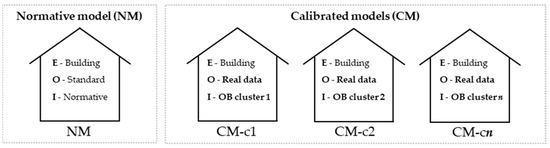
Figure 3.
Distribution of energy models and input data.
The simulation process runs the BPSs with the developed models and analyses the resulting outputs. As the study is focused exclusively on the heating energetic process, the study and simulation period is set from 1 December 2020 to 31 March 2021. Following the distribution of the models illustrated in Figure 3, one simulation processes the single NM, and n number of simulations process the diverse n number of CMs. As the result of the BPSs, the analysed resulting output are the hourly energy consumption of heating per area [kWh/m2] and the hourly mean dry bulb temperature [°C] for winter days (within the mentioned period). Afterwards, the analysis calculates the average hourly heating consumption and temperature during the days of each model’s studied winter season to describe the hourly energetic behaviour of each model. The results of this stage are the mean hourly consumption curve for heating in winter days [kWh/m2] and the mean hourly dry bulb temperature curve in winter days [°C].
2.3. Comparative Analysis
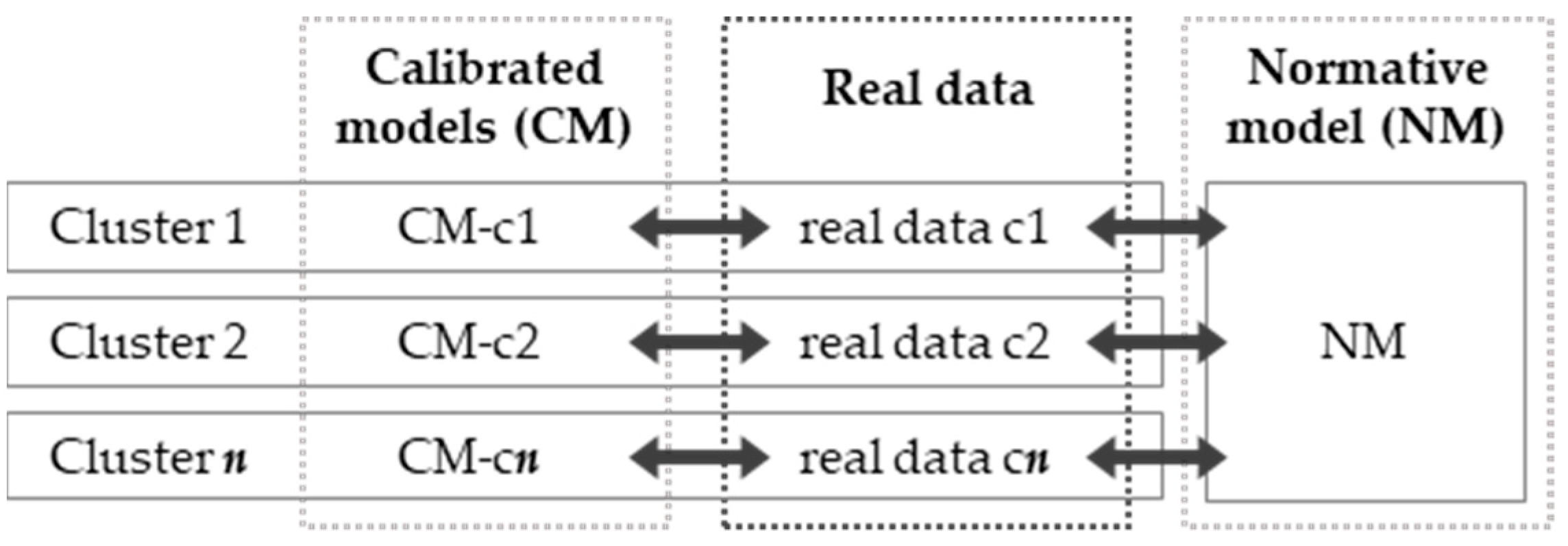
The third and last stage analyses the real monitored heating energy consumption and temperature as compared with the simulated heating energy consumption and temperature, both with the NM and CMs simulation outputs. The real data to compare are the monitored data applied in the calibration derived from the OB study developed in the previous study [32]; thus, the real data are organised in n clusters for the n OB profiles. The object of this stage is to compare analytically the real data of each OB cluster with their corresponding CM results of the same OB cluster and the NM results simultaneously, analysing the difference between the real data values of the CM and NM results, as shown in Figure 4. The compared data form the mean hourly heating consumption curve and the mean dry bulb temperature curve.
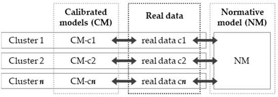
Figure 4.
Comparison scheme of real data with data from the calibrated models (CMs) by clusters and the normative model (NM).
The comparative analysis carries out an evaluation of the accuracy of both energy models, the NM and CMs, with the real data applying three statistical parameters:
- NMBE—Normalised mean bias error (Equation (1)): It provides the normalised mean bias error between the real data (r) and the simulated data (s) in percentage. The null value is the maximum accuracy of the simulated data concerning the real data, being positive or negative values as overestimated or underestimated predictions of the simulation data.
- CV-RMSE—Coefficient of variation of the root mean square error (Equation (2)): It provides the coefficient of error variability between the real data and simulated data normalised by the mean value. The null value is the maximum accuracy of the simulated data, rendering only positive values.
- CIF—Calibration improvement factor (Equation (3)): It provides the improvement ratio of the CM concerning the NM according to each of the two previous statistical p parameters (NMBE, CV-RMSE). The CIF indicates the gradient between the p statistical parameters (NMBE, CV-RMSE) of the NM and the CM in percentage. The positive value means an increase in the calibration accuracy, while the negative value means a decrease.
The statistical comparative parameters of NMBE and CV-RMSE compare the real data values with the CM and NM values for heating energy consumption and dry bulb temperature. These two statistical parameters (NMBE and CV-RMSE) have been applied in many previous studies to evaluate energy prediction models [16,33,34,35,36], as well as ASHRAE [37], IPMVP [38], and FEMP [39] guidelines. The CIF compares the values of the NMBE and CV-RMSE of the CM with those of the NM, measuring the improvement provided by the calibration in terms of NMBE and CV-RMSE.
3. Results
The methodology analyses a real case study of a social rental housing building located in Vitoria-Gasteiz, in the north of Spain, built in 2010. The building has 126 dwellings organised in two blocks of six and eight storeys. The heating system consists of a centralised natural gas boiler with radiators with individual control and no cooling system. The ventilation system is hybrid, with mechanical extraction in the kitchen and bathrooms and natural impulsion through windows with micro-ventilation combined with natural ventilation through windows. The building is located in a climatic zone categorised as Cfb, warm temperate, fully humid and warm summer, according to Köppen climate classification [40], and categorised as D climatic zone, according to the national regulations, the TBC [31].
3.1. Data Collection
The data collection follows the structure previously organised in the three-parameter groups (E, I, O) and the two types of models, the NM and CM. Moreover, the data have been collected according to the requirements of the modelling and simulation tool DesignBuilder [28] with the EnergyPlus calculation engine [29].
3.1.1. Envelope Factors (E)
The “building data” that describe the envelope factor come from the as-built construction project. This “building data” are the same for the NM and CM energy models. The building was built according to the 2007 version of the TBC [31], already with energy requirements, so the thermal envelope does have a high degree of thermal insulation. The envelope factor definition includes detailing all the material layers, with the thickness, thermal resistance, and thermal inertia of all the envelope elements, and the overall thermal transmittance (U value) and total thickness of each envelope element, as shown in Table 2. Moreover, the geometric distribution of the volume comes from the architecture plans of the mentioned project. Furthermore, the most critical thermal bridges have been taken into account and calculated by the finite elements calculation software Therm 7 [41], modelling and calculating the thermal bridges of the construction joints of façade–slab and façade–window–lintel as lineal thermal bridges (Ψ) [W/(m·K)], as detailed in Table 3.
Table 2.
Thermal envelope elements of the case study.
Table 3.
Thermal bridges of case study.
3.1.2. Outdoor Factors (O)
The outdoor factors are set according to the model type; for the NM standard data and CM, a new weather file was created with real data (see Table 4), as the NM applies the standard weather data for Vitoria-Gasteiz climatic data from 2007 and 2021 provided by IWEC directly in .epw format. The CMs apply the new weather file developed with climatic data monitored by the weather station located in Vitoria-Gasteiz (42.8604, −2.68899) managed by Euskalmet, the Basque meteorological agency. The climatic data is acquired from the open data platform of the Basque Government [42] to develop the .epw calibrated weather file. The climatic data used coincide with the study period to match the monitored real data and the simulation period, from 1 December 2020 to 31 March 2021.
Table 4.
Input data parameters for developing the NM and CMs of the case study.
3.1.3. Indoor Factors (I)
The data collection of the indoor factors includes two types of data, the “normative data” and “OB real data”. For the NM, only “normative data” are applied, based on the parameters defined in the CTE [31] in the energy-saving document named “Documento Básico de Ahorro de Energía”. The data collected in this source is relative to the thermal performance of the building, including the occupation density and schedule, the heating setpoint, setback and schedule, the ventilation flow and schedule, and other thermal gains (see Table 4). For the CMs, the study applies the “OB real data” corresponding to the real building obtained from monitoring and household surveys.
From the six clusters of OB obtained in the previous research [32], the average data of the dwellings in each cluster were taken for the parameters to be calibrated for the development of six CMs (see Table 4): the occupancy density (number of people/m2), the hourly occupancy schedule, heating setpoint and setback, and hourly heating schedule. Table 4 details the main input parameters for the NM and each of the six CMs, indicating the data source. The occupancy density defines the total number of people per area measured by surveys, and the occupancy schedule indicates the fraction of this total density during the day measured by the monitoring of CO2 concentration. The heating setpoint indicates the target temperature demanded by the heating system, and the setback indicates the minimum target temperature as a temporary lowering of the setpoint as an energy-saving strategy for non-active hours, like during the night. The heating schedule indicates the hourly use of heating, a value of 1.00 for the hours with the thermostat set in the setpoint temperature and 0.50 for the hours set in the setback temperature, calculated by the hourly energy consumption of the heating and monitoring of temperature. In the CMs, the input data regarding the ventilation and internal gains come from “normative data” due to the difficulty of accurately measuring this factor.
3.2. Energy Modelling and Building Performance Simulation
Firstly, the energy models are developed with the data collected in the previous stage in the software DesignBuilder v6 [28] (see Figure 5). On the one hand, one single NM is created with the “building data” as envelope factors, “standard weather data” as the outdoor factors, and “normative data” as the indoor factors. On the other hand, six CMs are created with the six OB clusters defined in the “OB real data” collection. For these CMs, the outdoor factors are defined by “real weather data”, the same data for all the CMs. However, for the indoor factors, the “OB real data” replace certain parameters with the corresponding OB cluster data for each CM (see Table 4). All the input data entry and the geometric volume are developed in DesignBuilder [28] following Table 4.

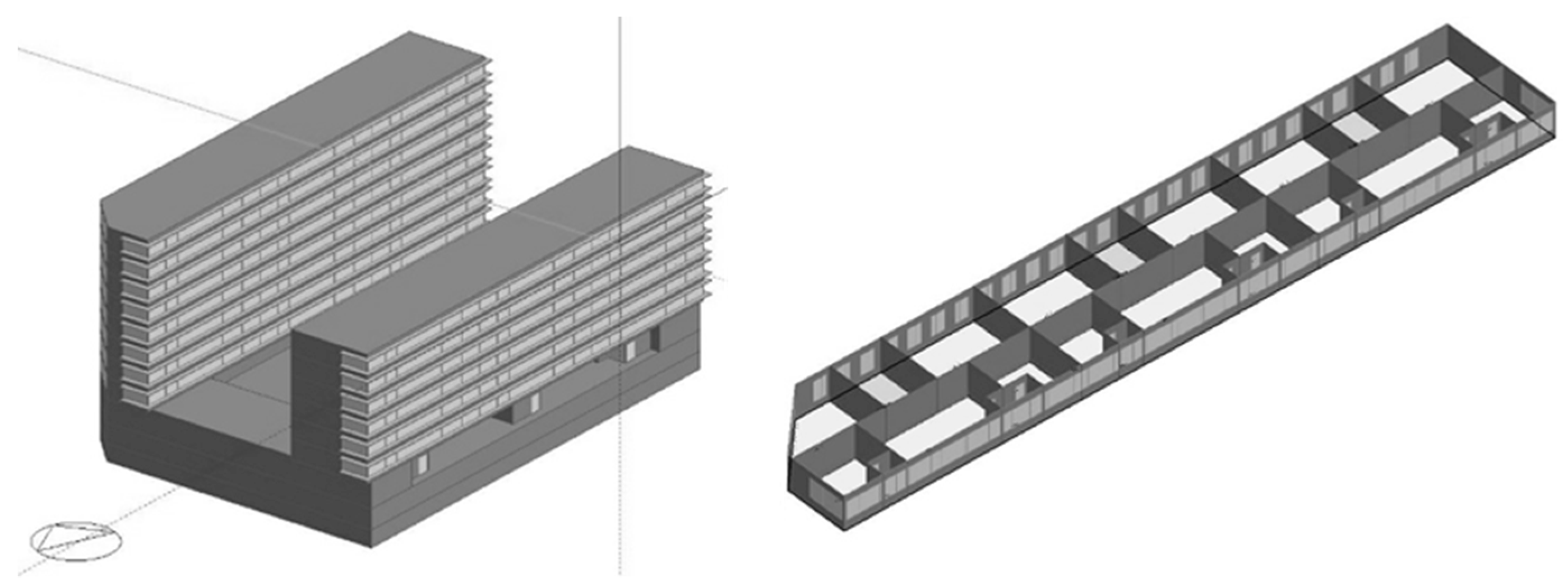
Figure 5.
Graphical representation of the model of the case study developed in DesignBuilder.
Secondly, the BPS is run for each energy model within the study period, running seven simulations, one for the NM and one for each of the six CMs. The output of the BPS is the hourly heating energy consumption and the indoor dry bulb temperature during the studied period (2094 h total). Table 5 shows the statistical summary of the results of the BPS together with the gross results of the monitored data as the real data measured in the previous study [32]. The table indicates the mean value, maximum value, minimum value, and standard deviation (SD) of the hourly energy consumption of heating per area [kWh/m2] and the hourly mean dry bulb temperature [°C]. Analysing the results, on the one hand, mean energy consumption of the BPS-based models, the NM and the six CMs, the results vary with the mean energy consumption between 11.54 and 15.20, five out of six CMs above the NM. However, when comparing the real data with the BPS-based data, the differences are much more significant, with real data mean energy consumption between 2.50 and 11.24. The lower values of the NM and CMs are much lower than the real data due to the non-uniform use of the household, so the computer model cannot represent it.
Table 5.
Statistical summary of the results of the energy simulations.
On the other hand, the temperature presents much less difference in the mean values, with some clusters with a higher average temperature and lower average energy consumption compared to the energy model. This is a clear indicator of an extra energy load, which can come from auxiliary heating systems like an electric or butane heater or a differing heat load of certain household uses, such as the use of the kitchen or other appliances. Furthermore, even if the SD of the temperature is significantly lower than in the energy data—and the average SD of the temperature is 0.91 against the SD of 10.56 for the energy consumption—the temperature real data also have a higher SD than the energy models. This is due to the same factor as in the energetic data, having a uniform behavioural pattern in the energy simulation and a lower uniformity in the real data, as the study predicts.
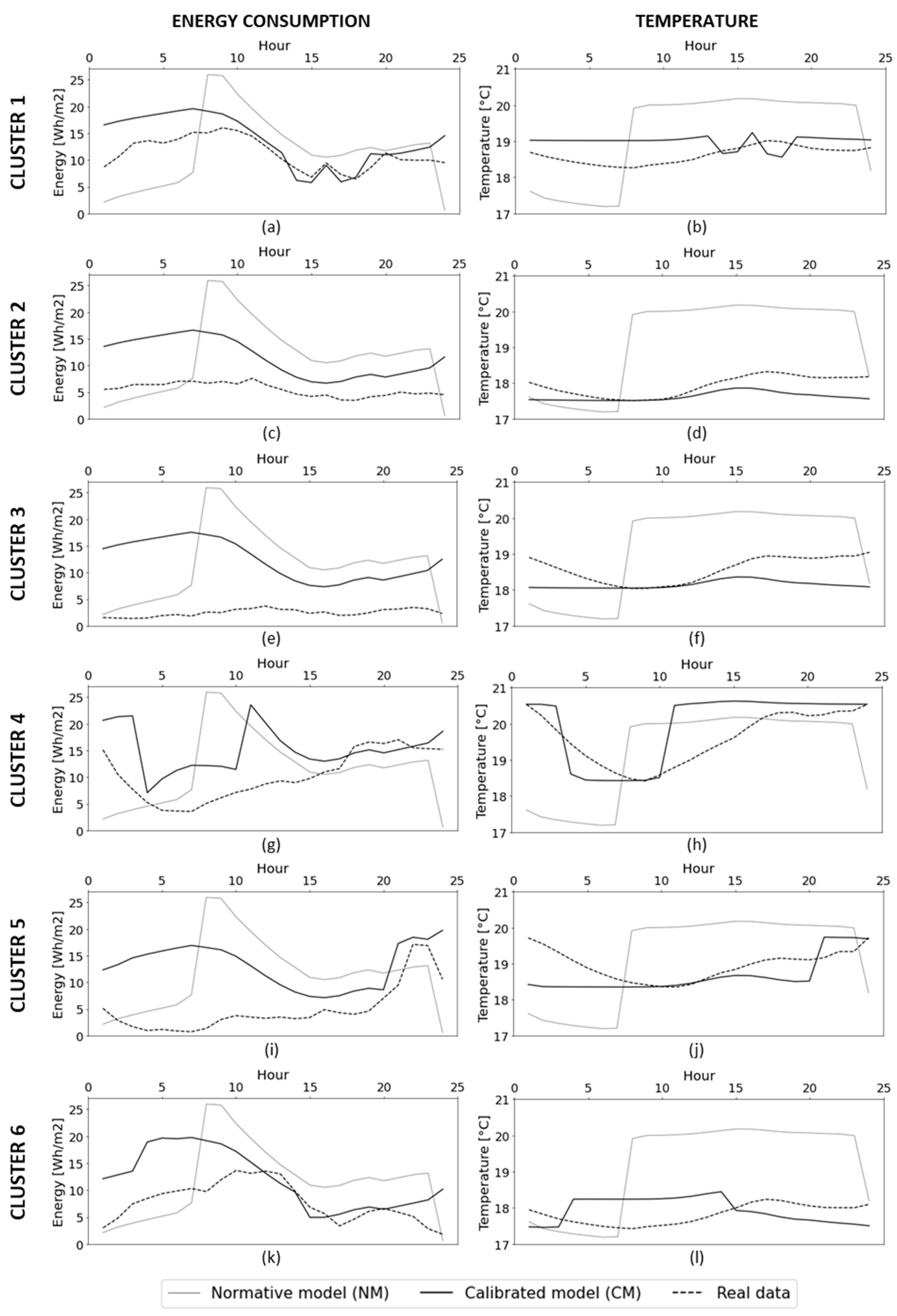
In order to enable the analysis of the building’s hourly thermal performance, this study calculates the mean hourly consumption curve for heating on winter days [kWh/m2] and the mean hourly dry bulb temperature curve [°C]. Figure 6 graphically shows the NM results for each OB cluster, the CM results of the corresponding cluster, and the real data obtained by the monitorization for heating energy consumption and indoor dry bulb temperature.

Figure 6.
Results of real data and simulated data from the calibrated model (CM) and the normative model (NM) of the mean hourly consumption curve for heating [kWh/m2] (a,c,e,g,i,k) and the mean hourly dry bulb temperature curve [°C] in winter days (b,d,f,h,j,l). and the mean hourly dry bulb temperature curve [°C] in winter days (b,d,f,h,j,l).
This interpretation allows us to make uniform the real data, building a behavioural model of the heating energy consumption and temperature for each cluster according to the CM and the real data, as well as the NM data. Firstly, Figure 6 indicates that the temperature data of the CM model fit much better with the real data than the energetic data, with a clear improvement in comparison with the NM data both in the shape of the curve and the values. Secondly, even if the energy consumption calculated by the CM does not fit with the real data as precisely as the temperature, it also shows an improvement in comparison with the NM, mainly in the shape of the curve. This can be due to the use of auxiliary heaters, where the increase or decrease of the energy consumption matches but with lower values in the real data; ergo, the main heating combines with an auxiliary heat load.
3.3. Comparative Analysis
For the quantitative comparative analysis of the real and simulated data through the NM and the CMs, the statistical analysis uses the parameters NMBE, CV-RMSE, and CIF (see Figure 7). The NMBE (in blue) of the NM indicates the error between the data from the NM and the measured real data of each cluster, and in the case of the CM, the error between the CM data and real data. The CV-RMSE (in yellow) of the NM indicates the variation of error comparing the NM data and real data of each cluster, and the CV-RMSE of the CM compares the CM data and real data. These indicators can measure the accuracy of the models, both NM and CMs. Furthermore, the CIF (in green) evaluates the improvement of the calibration of the CM in comparison with the NM according to the monitored real data, calculating the percentage improvement of the NMBE and CV-RMSE of each case, a higher value meaning a better improvement of the calibration process.
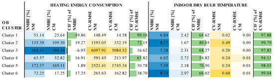
Figure 7.
Results of the statistical comparative parameters. NMBE is formatted in blues and CV-RMSE in yellows, where a darker colour means a higher error and less accuracy. CIF is formatted as a green bar diagram.
The results of Figure 7 gather three main points. Firstly, the calibrations acquire improved values of the NMBE and CV-RMSE, indicating a higher accuracy of the CMs compared to the NM, which the CIF numerically describes. Secondly, in all the cases, both the NM and CM achieve a higher accuracy for calculating the temperature than for the energy consumption and a higher improvement of the calibration. Thirdly, in terms of this calibration improvement, in both calculations of energy consumption and temperature, the CIF acquires higher values for the CV-RMSE than for the NMBE, indicating that the calibration offers a better improvement on the overall shape of the curve than the average error of this curve. In terms of variation between the OB clusters, the accuracy of the indoor temperature calculation is similar. The NMBE is between 6.02% and 8.74% for the NM and between 1.67% and 2.97% for the CM, with the CIF between 54% and 80%. Moreover, the CV-RMSE is also similar, with values around 0.015 and 0.595 for the NM and 0.001 and 0.014 for the CM, with the CIF between 94% and 99%.
4. Discussion
This research answers the need to cover the performance gap of BPS and the real energy behaviour of multi-family residential buildings by calibrating the OB patterns. The calibration is based on monitorization and survey data following the previous study by S. Perez-Bezos et al. [32], applying the diverse OB clusters that describe occupants’ occupancy and heating patterns. Therefore, this study offers a new approach to calibrating energy modelling and BPS of multi-family residential buildings with diverse OB patterns, focused on thermal behaviour in the winter season and heating process. Moreover, the calibration is completed with real weather data, and the BPS compares the normative data-based modelling, calibrated modelling, and measured real data based on a real case study of a social rental housing building located in Vitoria-Gasteiz, in the north of Spain.
This way, the study shows the current situation of calibrating energy models of collective residential buildings, considering OB’s existing diversity. As mentioned in the introductory section, many other studies of recent years have shown strong results in reducing the performance gap of BPS and real data, mainly in office buildings and single dwellings; however, the calibration to close the performance gap of multi-family residential buildings present other difficulties, barriers, and challenges on which this study is focused. Firstly, whereas the thermal losses and gains of the HVAC system can be measured, controlled, and simulated in office buildings, they are much more inaccurate in residential buildings. Tertiary buildings, unlike residential buildings, use mechanical ventilation with controlled ventilation rate and schedule with centralised HVAC systems that are the object of very accurate calibration studies [43,44,45]; however, these studies do not apply to residential buildings with natural ventilation and the HVAC resources fragmented in many appliances and thermal zones. Secondly, calibration processes carried out in tertiary buildings [12] and single dwellings [11] with homogeneous OB are considered to have a homogeneous thermal behaviour, which is different from the case of multi-family residential buildings with diverse OB patterns as demonstrated in the previous study by S. Perez-Bezos et al. [32].
Moreover, while other studies also applied parametric analyses to cover the uncertain parameters [46], the present study aims to reflect the OB by the BPS instead of obtaining exclusively low statistical errors, like the NMBE and CV-RMSE. The analyses and calculations obtained using these statistical parameters reflect an improvement of the results quantified by the CIF, meaning the positive value of the CIF renders a higher accuracy of the calibrated simulation in comparison with the one based on normative data in both mean hourly heating consumption and mean hourly dry bulb temperature in winter days (see Figure 7). Furthermore, these results achieved greater accuracy for temperatures rather than energy consumption with a higher CIF.
The results have shown many barriers in the calibration of energy modelling of residential buildings using monitored occupant behavioural data. The study has identified four main factors as barriers to optimal calibration. The first barrier is the difficulty of reflecting in an energy model the considerable diversity of usage behaviours in the residential building. Even if the OB diversity studied in the previous investigation [32] can be grouped and clustered, refining the OB patterns of the occupants, different OB clusters of the same building cannot be linked in one single energy model. Moreover, the connection between the socioeconomic conditions of the occupants and the OB patterns is not significant [32]. The second factor is the lack of uniformity and the fluctuation of OB patterns during the study period. These are difficult to analyse or predict and usually lead to a more significant deviation of the energy performance indicators like hourly energy consumption and temperature. This factor coincides with the more significant SD values of the measured real data compared to the simulated data of heating energy consumption and temperature (see Table 5). The third barrier is the uncertainty of several parameters linked to the heat losses and gains and the difficulty of analysing and simulating them, such as the natural ventilation and the quantification of heat gains of everyday operations of the residential buildings. Natural ventilation presents significant difficulties to measure and simulate in contrast to the mechanical ventilation managed by HVAC systems. Many studies have been able to measure, calibrate, and simulate the HVAC system, including the ventilation [44], but most studies that have studied natural ventilation remark many difficulties, where it has been shown possible to measure and simulate but only in one single dwelling [47].
Similarly, although the internal heat gains can be simulated precisely, the measurement of real data of heat gains presents difficulties, mostly related to domestic appliances with significant heat gains, such as from cooking and cleaning processes [48]. The last main barrier is the use of auxiliary heating systems that are not considered in the energy consumption of heating, which can be one of the main sources of heat gain [49]. The results of the study show that the calibrated data-based models have a higher accuracy in temperature calculation in comparison with the energy consumption of the main heating system (see Figure 6 and Figure 7), showing still a performance gap, which can be in part due to the use of secondary heating. Moreover, the results of the surveys of the previous study, which investigated the behavioural patterns of the case study [32], show that occupants reported the use of secondary heating systems even if this use was not quantified and could not be taken into account in the calibration. This factor can be significant in social housing, as in the case study of the present investigation, where the occupants instead use secondary heating appliances to concentrate the heating in a specific dwelling zone to reduce the energy cost [50].
Nevertheless, the identified four barriers can lead to opportunities for challenge. In the case of the first barrier of modelling the extensive diversity of OB of a building in one single model, the simulation of several OB clusters can determine a range of results that can be more precise than the results of a normative model. Moreover, a more profound survey process focused on the household’s behavioural patterns could help link each dwelling with an OB cluster, which could help develop an energy model divided into zones with different OB clusters. Concerning the difficulty of measuring and modelling natural ventilation, the use of window opening sensors can measure the level of ventilation [44], making it possible to link the ventilation rate for each OB cluster even if it is not precise. Furthermore, the heat gains of domestic appliances with significant energy use can be identified with the hourly energy consumption of the electricity.
In contrast, access to detailed hourly energy consumption data could be allowed in analysing the housing under public administration. Finally, the use of secondary heating systems could also be identified by analysing the hourly electricity consumption of electric heaters. However, heaters supplied by other energy sources—like butane or biomass—are challenging to quantify, but it is possible to identify their use by more precise surveys. Nevertheless, even if secondary heating systems are used, the model calculates the heating energy consumption based on the heating energy gain needed to achieve the calculated indoor temperature that demonstrates a high accuracy level.
The study’s limitations are aligned with the barriers and difficulties of the calibration of residential modelling with a significant diversity of OB. Firstly, the analysed sample in the OB cluster study was limited for optimal application in the whole building, where 54 out of 126 dwellings were studied by monitoring and surveys [32]. Secondly, the study did not monitor specific parameters, such as the window opening/closing as related to ventilation, the electricity consumption, or the surface temperatures of the façade, to detail the thermal transmittance of the envelope. Thirdly, the analysis of the use of heating considers the whole dwelling as one unit instead of monitoring the individual heaters. Consequently, the BPS considers the dwellings as one single thermal zone instead of zoning the residential unit into different rooms, which can have different thermal performances due to different OB patterns. Moreover, secondary heating systems are not analysed in alignment with one of the main barriers identified by monitoring these appliances’ electric consumption or with more detailed surveys. The previous study reported the use of secondary heating systems by surveys [32], but as it was not quantified, the study could not apply the use of secondary heating systems in the calibration process. Additionally, the study is exclusively focused on the study of heating energy behaviour, excluding other substantial energy-consuming end-uses such as domestic hot water (DHW) consumption. The main reason for not including DHW consumption is the lack of association between heating-consumption-related OB patterns and DWH consumption patterns identified by the previous study that developed the OB clusters [32]. In summary, the main limitations of the study and the main barriers identified in the calibration of modelling of residential with significant diversity of OB come down to data collection.
Our study suggests more profound data collection in terms of the energetic behaviour of occupants in order to reach a higher degree of accuracy in the calibration of residential building energy models. As a future research avenue, on the one hand, a more detailed OB analysis should be performed by monitoring and surveys, focusing on the heat loss and gains such as ventilation, use of heating, and other heat gains caused by high-energy appliances. Additionally, the influence of DHW consumption can also be taken into account to cover a larger share of total energy consumption of households, as recent studies found discrepancies between real and standard values of DHW consumption [51]. Moreover, monitoring ventilation patterns like the opening/closing of windows can develop a more detailed model through computational fluid dynamics (CFD) models, relating the OB clusters with ventilation patterns. On the other hand, the parametric modelling of the OB patterns can provide a range of results covering the likely real energy performance. Furthermore, the authors consider parametric modelling valuable for providing a range of results instead of one single number as the definitive result, but not for identifying uncertain parameters. However, the parametric study can also be an excellent resource to identify the most influential parameters to monitor or study.
5. Conclusions
The current study investigates the opportunities and barriers to calibrating collective residential building energy modelling by occupant behavioural real data focused on the analysis of heating energy consumption. For this, the study develops one model based on normative input data and diverse calibrated models based on OB clusters defined in a previous investigation in a real case study of a social rental housing building. The statistical analysis shows a significant improvement of the simulated hourly indoor dry bulb temperature, with an average improvement of 67% in the NMBE and 98% in the CV-RMSE; the improvement of the hourly heating energy consumption is 16% in the NMBE and 52% in the CV-RMSE. These results show the main findings of the study.
On the one hand, the considerable diversity of OB is a barrier to developing one single OB pattern that fits all users. However, a set of OB clusters can provide a diverse range of energy performance results, where a deeper survey-based study could improve the accuracy of these OB clusters and their results in an energy simulation. Ergo, the calibration method based on OB clustering brings significant improvements in data accuracy at the hourly level, making this approach an opportunity for calibration techniques.
On the other hand, the higher improvement of the temperature simulation with higher values of simulated energy consumption indicates the existence of higher heat gains that can be caused by auxiliary heating systems and other gains that have not been monitored and modelled, showing the main research barriers. This further suggests other difficulties in measuring specific OB parameters, such as the mentioned heat gains and use of auxiliary heating systems, but also other OB-related parameters like the ventilation flow. Nevertheless, this can be challenged by deeper monitoring and surveys, covering a wider range of OB-related parameters.
To conclude, the study provides a new approach to calibrating collective residential building energy models with OB diversity towards minimising the performance gap, reflecting the reality of a diversity of OB patterns. The proposed methodology presents considerable replicability in other residential buildings and socioeconomic contexts, focusing on the identified challenges. The method makes it possible to obtain the results of energy performance in a range of values, covering a wide range of diverse OB patterns and a more significant part of reality.
Author Contributions
Conceptualization, M.A., A.F.-L. and X.O.; Methodology, M.A., S.P.-B. and A.F.-L.; Validation, X.O.; Formal analysis, M.A. and S.P.-B.; Investigation, M.A., S.P.-B. and A.F.-L.; Resources, S.P.-B.; Data curation, M.A. and S.P.-B.; Writing—original draft, M.A., S.P.-B. and A.F.-L.; Writing—review & editing, A.F.-L. and X.O.; Visualization, M.A.; Supervision, X.O. All authors have read and agreed to the published version of the manuscript.
Funding
The thesis of Silvia Perez-Bezos is funded by the Call for tender for a researcher training at the University of the Basque Country UPV/EHU 2019 (PIF19/139) and the thesis of Markel Arbulu is funded by the Predoctoral Training Programme for Non-Doctor Research Personnel of the Department of Education of the Basque Government (PRE_2022_2_0121). This research is also funded by the grants to support research groups of the university system of the Basque Government awarded to CAVIAR research group (GIC21/161).
Institutional Review Board Statement
Ethics approval from the Ethics Committee for Research on Human Subjects, CEISH-UPV/EHU, BOPV 32, 17/2/2014, was obtained prior to conducting the study.
Data Availability Statement
The data presented in this study are available on request from the corresponding author.
Acknowledgments
The authors would like to acknowledge the Public Society Alokabide and the company STECHome for their support and contribution and for the information, access, and monitoring data provided. This research work will form part of three doctoral theses carried out by Silvia Perez-Bezos, Markel Arbulu, and Anna Figueroa-Lopez.
Conflicts of Interest
The authors declare no conflicts of interest.
References
- Pan, Y.; Zhu, M.; Lv, Y.; Yang, Y.; Liang, Y.; Yin, R.; Yang, Y.; Jia, X.; Wang, X.; Zeng, F.; et al. Building energy simulation and its application for building performance optimization: A review of methods, tools, and case studies. Adv. Appl. Energy 2023, 10, 100135. [Google Scholar] [CrossRef]
- European Union. Directive (EU). 2024/1275 of the European Parliament and of the Council of 24 of April 2024. Available online: https://eur-lex.europa.eu/legal-content/EN/TXT/?uri=OJ:L_202401275&pk_keyword=Energy&pk_content=Directive (accessed on 1 June 2023).
- Chong, A.; Gu, Y.; Jia, H. Calibrating building energy simulation models: A review of the basics to guide future work. Energy Build. 2021, 253, 111533. [Google Scholar] [CrossRef]
- Winkelmann, F.C.; Birdsall, B.E.; Buhl, W.F.; Ellington, K.L.; Erdem, A.E.; Hirsch, J.J.; Gates, S. DOE-2 Supplement: Version 2.1E; Lawrence Berkeley National Lab. (LBNL): Berkeley, CA, USA; Hirsch (James J.) and Associates: Camarillo, CA, USA, 1993. [CrossRef]
- Crawley, D.B.; Lawrie, L.K.; Winkelmann, F.C.; Buhl, W.F.; Huang, Y.J.; Pedersen, C.O.; Strand, R.K.; Liesen, R.J.; Fisher, D.E.; Witte, M.J.; et al. EnergyPlus: Creating a new-generation building energy simulation program. Energy Build. 2001, 33, 319–331. [Google Scholar] [CrossRef]
- Klein, S.A.; Beckman, W.A. TRNSYS 16: A Transient System Simulation program: Mathematical Reference—Volume 5. Trnsys 2007, 5, 389–396. [Google Scholar]
- ESRU. The ESP-r System for Building Energy Simulation: User Guide Version 10 Series; University of Strathclyde: Glasgow, Scotland, 2002; p. 63. [Google Scholar]
- Coleman, S.; Touchie, M.F.; Robinson, J.B.; Peters, T. Rethinking performance gaps: A regenerative sustainability approach to built environment performance assessment. Sustainability 2018, 10, 4829. [Google Scholar] [CrossRef]
- Sunikka-Blank, M.; Galvin, R. Introducing the prebound effect: The gap between performance and actual energy consumption. Build. Res. Inf. 2012, 40, 260–273. [Google Scholar] [CrossRef]
- Cozza, S.; Chambers, J.; Deb, C.; Scartezzini, J.L.; Schlüter, A.; Patel, M.K. Do energy performance certificates allow reliable predictions of actual energy consumption and savings? Learning from the Swiss national database. Energy Build. 2020, 224, 110235. [Google Scholar] [CrossRef]
- Cuerda, E.; Guerra-Santin, O.; Sendra, J.J.; Neila, F.J. Understanding the performance gap in energy retrofitting: Measured input data for adjusting building simulation models. Energy Build. 2020, 209, 109688. [Google Scholar] [CrossRef]
- Coakley, D.; Raftery, P.; Keane, M. A review of methods to match building energy simulation models to measured data. Renew. Sustain. Energy Rev. 2014, 37, 123–141. [Google Scholar] [CrossRef]
- ASHRAE. Measurement of Energy, Demand, and Water Savings. In ASHRAE Guideline 14-2014; ASHRAE: Peachtree Corners, GA, USA, 2014. [Google Scholar]
- Bhandari, M.; Shrestha, S.; New, J. Evaluation of weather datasets for building energy simulation. Energy Build. 2012, 49, 109–118. [Google Scholar] [CrossRef]
- ANSI; ASHRAE. ASHRAE Guideline 14—2002 Measurement of Energy and Demand Savings. Ashrae 2002, 8400, 170. [Google Scholar]
- Ruiz, G.; Bandera, C. Validation of Calibrated Energy Models: Common Errors. Energies 2017, 10, 1587. [Google Scholar] [CrossRef]
- Efficiency Valuation Organization. International Performance Measurement and Verification Protocol; Efficiency Valuation Organization (EVO): Washington, DC, USA, 2023. [Google Scholar]
- US Department of Energy. M&V Guidelines: Measurement and Verification for Federal Energy Projects Version 2.2; Lawrence Berkeley National Laboratory: Berkeley, CA, USA, 2008.
- Chen, S.; Zhang, G.; Xia, X.; Chen, Y.; Setunge, S.; Shi, L. The impacts of occupant behavior on building energy consumption: A review. Sustain. Energy Technol. Assess. 2021, 45, 101212. [Google Scholar] [CrossRef]
- Charlier, D. Explaining the energy performance gap in buildings with a latent profile analysis. Energy Policy 2021, 156, 112480. [Google Scholar] [CrossRef]
- van den Brom, P.; Meijer, A.; Visscher, H. Performance gaps in energy consumption: Household groups and building characteristics. Build. Res. Inf. 2018, 46, 54–70. [Google Scholar] [CrossRef]
- D’Oca, S.; Gunay, H.B.; Gilani, S.; O’Brien, W. Critical review and illustrative examples of office occupant modelling formalisms. Build. Serv. Eng. Res. Technol. 2019, 40, 732–757. [Google Scholar] [CrossRef]
- Guerra-Santin, O.; Bosch, H.; Budde, P.; Konstantinou, T.; Boess, S.; Klein, T.; Silvester, S. Considering user profiles and occupants’ behaviour on a zero energy renovation strategy for multi-family housing in the Netherlands. Energy Effic. 2018, 11, 1847–1870. [Google Scholar] [CrossRef]
- Cuerda, E.; Guerra-Santin, O.; Sendra, J.J.; Neila González, F.J. Comparing the impact of presence patterns on energy demand in residential buildings using measured data and simulation models. Build. Simul. 2019, 12, 985–998. [Google Scholar] [CrossRef]
- Salvia, G.; Morello, E.; Rotondo, F.; Sangalli, A.; Causone, F.; Erba, S.; Pagliano, L. Performance gap and occupant behavior in building retrofit: Focus on dynamics of change and continuity in the practice of indoor heating. Sustainability 2020, 12, 5820. [Google Scholar] [CrossRef]
- Mahecha Zambrano, J.; Filippi Oberegger, U.; Salvalai, G. Towards integrating occupant behaviour modelling in simulation-aided building design: Reasons, challenges and solutions. Energy Build. 2021, 253, 111498. [Google Scholar] [CrossRef]
- Eurostat. Disaggregated Final Energy Consumption in Households—Quantities. Available online: https://ec.europa.eu/eurostat/databrowser/view/nrg_d_hhq/default/table?lang=en (accessed on 31 August 2023).
- Design Builder. Design Builder Simulation Tool. 2022. Available online: https://designbuilder.co.uk/ (accessed on 1 June 2023).
- U.S. Department of Energy’s (DOE) Building Technologies Office (BTO). Energy Plus Energy Simulation Tool. 2001. Available online: https://energyplus.net/ (accessed on 1 June 2023).
- ASHRAE. International Weather Files for Energy Calculations 2.0 (IWEC2). 2012. Available online: https://www.ashrae.org/technical-resources/bookstore/ashrae-international-weather-files-for-energy-calculations-2-0-iwec2 (accessed on 1 June 2023).
- Ministerio de Transportes Movilidad y Agenda Urbana. Gobierno de España. CTE—Código Técnico de la Edificación. 2019. Available online: https://www.codigotecnico.org/ (accessed on 1 June 2023).
- Perez-Bezos, S.; Guerra-Santin, O.; Grijalba, O.; Hernandez-Minguillon, R.J. Occupants’ behavioural diversity regarding the indoor environment in social housing. Case study in Northern Spain. J. Build. Eng. 2023, 77, 107290. [Google Scholar] [CrossRef]
- Ciulla, G.; D’Amico, A. Building energy performance forecasting: A multiple linear regression approach. Appl. Energy 2019, 253, 113500. [Google Scholar] [CrossRef]
- Yun, K.; Luck, R.; Mago, P.J.; Cho, H. Building hourly thermal load prediction using an indexed ARX model. Energy Build. 2012, 54, 225–233. [Google Scholar] [CrossRef]
- Chae, Y.T.; Horesh, R.; Hwang, Y.; Lee, Y.M. Artificial neural network model for forecasting sub-hourly electricity usage in commercial buildings. Energy Build. 2016, 111, 184–194. [Google Scholar] [CrossRef]
- Yezioro, A.; Dong, B.; Leite, F. An applied artificial intelligence approach towards assessing building performance simulation tools. Energy Build. 2008, 40, 612–620. [Google Scholar] [CrossRef]
- ASHRAE. Guideline 14-2014: Measurement of Energy, Demand, and Water Savings. 2014. Available online: https://webstore.ansi.org/standards/ashrae/ashraeguideline142014 (accessed on 1 June 2023).
- IPMVP. Concepts and Options for Determining Energy and Water Savings. 2002. Available online: https://www.nrel.gov/docs/fy02osti/31505.pdf (accessed on 1 June 2023).
- FEMP. M&V Guidelines: Measurement and Verification for Performance-Based Contracts. 2015. Available online: https://www.energy.gov/node/1413841 (accessed on 1 June 2023).
- Beck, H.E.; Zimmermann, N.E.; McVicar, T.R.; Vergopolan, N.; Berg, A.; Wood, E.F. Present and future Köppen-Geiger climate classification maps at 1-km resolution. Sci. Data 2018, 5, 180214. [Google Scholar] [CrossRef] [PubMed]
- Lawrence Berkeley National Laboratory. Therm 7 Software; version 7; U.S. Department of Energy National Laboratory: Livermore, CA, USA, 2017.
- Basque Government. Open Data Euskadi. 2023. Available online: https://opendata.euskadi.eus/ (accessed on 4 August 2023).
- Li, G.; Xiong, J.; Sun, S.; Chen, J. Validation of virtual sensor-assisted Bayesian inference-based in-situ sensor calibration strategy for building HVAC systems. Build. Simul. 2023, 16, 185–203. [Google Scholar] [CrossRef]
- Zhang, Z.; Chong, A.; Pan, Y.; Zhang, C.; Lam, K.P. Whole building energy model for HVAC optimal control: A practical framework based on deep reinforcement learning. Energy Build. 2019, 199, 472–490. [Google Scholar] [CrossRef]
- Palaić, D.; Štajduhar, I.; Ljubic, S.; Wolf, I. Development, Calibration, and Validation of a Simulation Model for Indoor Temperature Prediction and HVAC System Fault Detection. Buildings 2023, 13, 1388. [Google Scholar] [CrossRef]
- Manfren, M.; James, P.A.; Tronchin, L. Data-driven building energy modelling—An analysis of the potential for generalisation through interpretable machine learning. Renew. Sustain. Energy Rev. 2022, 167, 112686. [Google Scholar] [CrossRef]
- Aparicio-Fernández, C.; Vivancos, J.-L.; Cosar-Jorda, P.; Buswell, R.A. Energy Modelling and Calibration of Building Simulations: A Case Study of a Domestic Building with Natural Ventilation. Energies 2019, 12, 3360. [Google Scholar] [CrossRef]
- Bansal, P.; Vineyard, E.; Abdelaziz, O. Advances in household appliances—A review. Appl. Therm. Eng. 2011, 31, 3748–3760. [Google Scholar] [CrossRef]
- Nishimwe, A.M.R.; Reiter, S. Building heat consumption and heat demand assessment, characterization, and mapping on a regional scale: A case study of the Walloon building stock in Belgium. Renew. Sustain. Energy Rev. 2021, 135, 110170. [Google Scholar] [CrossRef]
- Mahdavi, A.; Berger, C.; Amin, H.; Ampatzi, E.; Andersen, R.K.; Azar, E.; Barthelmes, V.M.; Favero, M.; Hahn, J.; Khovalyg, D.; et al. The Role of Occupants in Buildings’ Energy Performance Gap: Myth or Reality? Sustainability 2021, 13, 3146. [Google Scholar] [CrossRef]
- Ratajczak, K.; Michalak, K.; Narojczyk, M.; Amanowicz, Ł. Real Domestic Hot Water Consumption in Residential Buildings and Its Impact on Buildings’ Energy Performance—Case Study in Poland. Energies 2021, 14, 5010. [Google Scholar] [CrossRef]


Disclaimer/Publisher’s Note: The statements, opinions and data contained in all publications are solely those of the individual author(s) and contributor(s) and not of MDPI and/or the editor(s). MDPI and/or the editor(s) disclaim responsibility for any injury to people or property resulting from any ideas, methods, instructions or products referred to in the content. |
© 2024 by the authors. Licensee MDPI, Basel, Switzerland. This article is an open access article distributed under the terms and conditions of the Creative Commons Attribution (CC BY) license (https://creativecommons.org/licenses/by/4.0/).