Abstract
The discrete time-cost tradeoff problem (DTCTP) is a well-researched topic in the field of operations research. The majority of existing DTCTP models are based on traditional activity networks, which permit the execution of an activity as soon as all its predecessors have been completed. This assumption is reasonable, but it is important to note that there are always exceptions. The main work of this study was threefold. Firstly, we expanded the analysis of the DTCTP to encompass time-constrained activity networks (DTCTPTC), which encompassed three different types of time constraints. The first constraint was the time-window constraint, which limited the time interval during which an activity could be executed. The second constraint was the time-schedule constraint, which specified the times at which an activity could begin execution. The third constraint was the time-switch constraint, which required project activities to start at specific times and remain inactive during designated time periods. Secondly, a constraint programming (CP) model was developed for the purpose of solving the DTCTPTC. The model employed interval variables to define the activity and its potential time constraints, while CP expressions were utilized to ensure the feasibility of the solution. The objective was to identify the optimal execution mode for each activity, the optimal start times for time-scheduled activities, and the optimal work/rest patterns for time-switch activities, with the aim of minimizing the total cost of the project. Finally, the efficacy of the proposed CP model was validated through two case studies based on two illustrative projects of varying sizes. The outcomes were then compared against existing algorithms. The results demonstrated that time constraints were important factors affecting schedule optimization, and the proposed CP model had the ability to solve large-scale DTCTPTC.
1. Introduction
The time–cost tradeoff problem (TCTP) has been extensively studied in project scheduling literature and is crucial for optimizing resource allocation [1]. A TCTP is defined by a set of activities and their precedence relationships. Each activity has a duration (processing time) that can be shortened by additional funds. The objective is to determine the optimal time–cost tuple for each activity to achieve the desired goals. Due to the discrete nature of many resources, such as workers and machines [2], research has focused on the discrete variant of the TCTP, known as the discrete time–cost tradeoff problem (DTCTP). The DTCTP arises when the duration of an activity is a discrete, non-increasing function of the amount of money invested in it. In this context, the set of alternative modes for an activity consisted of all possible time–cost combinations.
In literature, the DTCTP has been studied in three categories: the deadline problem, the budget problem, and the time–cost curve problem [3]. The deadline problem aims to minimize the total project cost for all mode assignments without exceeding a given deadline. The budget problem seeks to minimize the project duration subject to a constraint that limits the budget for the total project cost. The problem of constructing a complete and efficient time–cost profile over feasible project durations is known as the time–cost curve problem. This curve can be found using a horizon-varying approach, which involves iteratively solving the deadline problem over feasible project durations. De et al. [4] demonstrated that all three categories of the DTCTP are NP-hard in the strong sense. Accordingly, it cannot be expected that exact algorithms will terminate within a reasonable amount of time. The remainder of this paper analyzes the deadline version of the DTCTP.
Numerous studies have been conducted on the DTCTP with varying objectives and constraints due to its practical relevance. However, meeting the demands of project management still presents some challenges. Particularly, existing DTCTP models are primarily based on a traditional activity network that permits an activity to be executed once all of its predecessors have been completed. This approach is reasonable, but it may not cover all possible real-life situations. For instance, consider a typical workday (Monday to Friday) where employees work from 9 a.m. to 12 p.m. and from 1 p.m. to 5 p.m. In this case, an activity may have time constraints that require it to be inactive during specific time intervals. To model these situations in project management, researchers have identified and investigated three common types of time constraints [5,6,7]. The first is the time-window constraint, which limits an activity to a specific time interval. A time window specifies the earliest and latest times that an activity can be active after its preceding activities are completed. The time-schedule constraint forces an activity to start at one of the ordered schedule’s beginning times. Therefore, an activity can only begin execution after all its predecessors are completed and at one of the beginning times in the time schedule. The third constraint is the time-switch constraint, which assumes that time can be treated as repeating cycles. Each cycle consists of pairs of work and rest windows. Activities can only be performed during work windows, and their execution must be interrupted during rest windows.
In the current competitive environment, it is common for contractors and planners to accelerate project delivery by performing time–cost tradeoff optimizations at the activity level. To ensure effective and accurate solutions, all factors that may influence optimization results should be considered. Failure to consider time constraints in time–cost tradeoff optimization can result in inaccurate planning and scheduling, potentially leading to problematic solutions. Specifically, the project durations of these solutions may be longer than expected due to time constraints on critical activities. Furthermore, these solutions may become impractical due to unmet time constraints. Finally, even if these solutions remain valid when time constraints are considered, the earliest start and the latest finish times of each activity may be estimated incorrectly. Therefore, it is crucial to take time constraints into account when implementing a time–cost tradeoff optimization.
This paper investigates the DTCTP in a time-constrained activity network (abbreviated as the DTCTPTC), which includes three types of time constraints. The DTCTPTC is an extension of the DTCTP and involves complex combinatorial optimization. To address the computational challenges, this paper develops an efficient scheduling optimization model based on constraint programming (CP). CP has been shown to be an efficient solution technique for solving many combinatorial optimization problems [8]. It has gained significant attention in the research community due to its flexibility and effectiveness.
The remainder of the paper is organized as follows. In Section 2, the relevant research on time–cost tradeoffs is reviewed. In Section 3, a concise overview of the CP methodology is provided. In Section 4, the DTCTPTC is defined, and the proposed CP model is formulated. In Section 5, two illustrated projects of varying sizes are used to verify the efficacy of the proposed CP model. In Section 6, a sensitivity analysis of the key parameters of the proposed model is conducted, and a comparison with existing algorithms is performed. Finally, concluding remarks and future research directions are discussed in Section 7.
2. Literature Review
Methods for solving the TCTP and DTCTP can be classified into exact algorithms and heuristic procedures. Exact algorithms are typically based on integer programming and the branch-and-bound method, but they struggle to solve large and complex instances measured in terms of the number of activities, the structure of the project networks, and the number of modes per activity [9]. Hafızoğlu and Azizoğlu [10] proposed an exact algorithm and a heuristic procedure to address the DTCTP using the linear programming relaxation idea. The heuristic procedure employs an initial solution generated by construction heuristics, which are then refined through single and pairwise interchanges, resulting in rapid solution generation. Klanšek and Pšunder [11] presented a mixed-integer nonlinear programming (MINLP) model for the DTCTP with a nonlinear objective function for total project cost. The MINLP model handles the discrete variables explicitly and does not require the rounding of the continuous solution into an integer solution. Szmerekovsky and Venkateshan [12] proposed a new integer programming formulation for the irregular costs project scheduling problem with time–cost tradeoffs. Empirical tests have demonstrated that, in numerous instances, the new formulation performs optimally and can resolve problems with up to 90 activities in a reasonable amount of time. Choi and Kang [13] developed a strongly polynomial time algorithm for a linear TCTP with multiple milestones under a comb graph. This graph represents a chain of jobs that sequentially precede each other, forming the main process of a project. Other chains of jobs, corresponding to subprocesses, precede each job in the main process. The objective of this algorithm is to minimize the weighted number of tardy milestones plus the total compression cost. Aouam and Vanhoucke [14] conducted a study on a multi-mode project scheduling problem from an agency perspective. In this context, agency refers to the risk-averse contractor’s hidden effort, which influences the duration and cost of project activities. They formulated the owner’s problem as a bi-level program, where the lower level involves a TCTP. Eynde and Vanhoucke [15] developed an exact DTCTP algorithm based on the network reduction approach. They introduced a new data structure called the reduction tree to track the modular decomposition structure. Nasiri and Lu [16] presented a streamlined optimization algorithm to implement TCTP analysis, allowing for the identification of local and global optimums in an analytical and automated fashion. Wang et al. [17] noted that the algorithm faces challenges with high memory requirements and computational demands in complex, large-scale projects involving tens of millions of paths and hundreds of activities. They suggested a modified streamlined optimization algorithm to address these challenges. Daboul et al. [18] analyzed a specific case of the DTCTP with a constant upper bound on the number of activities in any path. They developed a simple approximation algorithm for such instances, which could occur in VLSI design.
Due to the phenomenon of combinatorial explosion, heuristic algorithms are commonly used to handle the DTCTP by searching for optimal or acceptable approximate solutions. Aminbakhsh and Sonmez [2] presented a discrete particle swarm optimization (DPSO) to achieve an effective method for the large-scale DTCTP involving up to 630 activities. The DPSO is based on novel principles for the representation, initialization, and position updating of particles. It offers several benefits for solving the DTCTP, including an adequate representation of the discrete search space and enhanced optimization capabilities due to an improved quality of the initial swarm. Alavipour and Arditi [19] proposed an integrated model based on genetic algorithm (GA) and linear programming to solve the DTCTP considering financing costs, with the objective of minimizing total cost and maximizing profit. Togan and Eirgas [20] designed a new approach for the initial population of the teaching learning-based DTCTP algorithm. The aim was to reduce randomness in the initial population and decrease the search effort required to find the optimal set of time–cost alternatives in the search space. Banihashemi et al. [21] used fuzzy multi-criteria decision-making methods to solve a discrete time–cost–quality tradeoff problem. The authors applied the SWARA method to determine the weights of time, cost, and quality. Then, they used the TOPSIS technique to select the best activity modes. Gupta and Trivedi [22] proposed an Apriori-based elephant herding optimization (EHO) method for time–cost tradeoff optimization. The method utilizes the Apriori algorithm to generates the rules on the input parameters and then applies the EHO algorithm to those input parameters. Bettemir and Birgonul [23] developed a hybrid heuristic meta-heuristic algorithm to solve the large-scale DTCTP. The algorithm uses a minimum cost slope-based heuristic network analysis algorithm to eliminate the infeasible search domain. To reduce the possibility of the meta-heuristic algorithm converging into local minima, an adaptive search domain approach is employed. Son and Nguyen Dang [24] proposed a hybrid model, the multi-verse optimizer combined with the sine cosine algorithm, to address the DTCTP.
Similarly, various authors have explored expansions of the DTCTP. El-Rayes and Kandil [25] examined the problem of discrete-time–cost–quality tradeoff and created a method based on multi-objective GA. Cheng and Tran [26] presented an opposition-based multi-objective differential evolution for the time–cost–environmental tradeoff problem. The algorithm utilized an opposition-based learning technique for population initialization and generation jumping. Mohammadipour and Sadjadi [27] addressed the discrete cost–quality–risk tradeoff problem with a deadline constraint and presented a multi-objective mixed-integer linear programming (MILP) model. The goal attainment method was employed in order to resolve the multi-objective model and to identify the Pareto-optimal solutions. Hariga et al. [28] investigated integrated time–cost tradeoff and resource leveling problems while considering allowed activity splitting. The formulated MILP model considers the tradeoff between the crashing-dependent costs, direct and indirect costs, and resource utilization-related costs, and acquiring, releasing, and splitting costs. Heravi and Moridi [29] analyzed time–cost tradeoffs for resource-constrained repetitive projects. They utilized a time-variant multi-objective PSO to identify non-dominated solutions that minimize time and cost. Banihashemi et al. [30] developed a multi-objective optimization model for the discrete tradeoff problem of time, cost, quality, and environmental impacts in project implementation. The aim of the multi-objective model is to minimize time, cost, and environmental impacts while maximizing project quality. Chen et al. [31] analyzed a new hierarchical DTCTP in multi-project scenarios and proposed a program to manage multiple related projects. The program at the upper layer is responsible for allocating budgets and targets to projects at the lower layer. Each project is scheduled independently, with the scheduling results at the lower layer being fed back to the program for further coordination and optimization. Yazdani et al. [32] addressed the DTCTP with discounted cash flows. The objective was to maximize the net present value of cash flows by selecting execution modes for activities while considering project deadlines. To solve the problem, they employed the generalized benders decomposition technique. Further research on the integration of other optimization objectives into the DTCTP can be found in Hosseinzadch et al. [33], Mahdiraji et al. [34], and Lotfi et al. [35].
In addition, several studies have focused on variants of the DTCTP in uncertain environments. For instance, Abdel-Basset et al. [36] designed a framework to handle time–cost tradeoffs while considering the real and uncertain situation surrounding the projects. The framework used trapezoidal neutrosophic numbers to estimate the durations of activities, and the goal was to minimize the costs of projects under uncertain environmental conditions. Godinho and Costa [37] established a stochastic model for the DTCTP, where the activity can be performed by using several different resources, and the resource used can change depending on how the activity evolves. Tao et al. [38] proposed a time–cost tradeoff model in GERT networks. In order to ensure successful project completion, constraints were added to the probability of on-time delivery and under-budget. A genetic algorithm-based solution procedure was then designed to solve the tradeoff model. Lotfi et al. [39] investigated the time–cost–quality–energy–environment problem under uncertainty and presented a robust nonlinear programming model that includes the objectives of cost, quality, energy, and pollution levels. Li et al. [40] developed an epsilon-constraint method-based GA along with three improvement measures to address a discrete time–cost–robustness tradeoff problem in uncertain environments. Mahdavi-Roshan and Mousavi [41] presented a new project scheduling model that considers resource constraints and tradeoffs between time, cost, and quality. To handle uncertainty, they used interval-valued fuzzy sets for several parameters and developed a new hybrid solution approach for the interval-valued fuzzy mathematical model. In addition, Kostrzewa-Demczuk [42] proposed a Probabilistic Time Coupling Method (PTCM) for determining the minimum, most probable, and maximum time required for project implementation. The PTCM enables the use of forecast data based on the actual course of work similar to planned work performed in the past, which reflects real conditions accurately.
The literature on the DTCTP and its extensions is extensive. However, only a few studies have addressed the DTCTP with time constraints. Vanhoucke et al. [43] described an exact branch-and-bound algorithm and a heuristic procedure for the DTCTP involving three special cases of time-switch constraints: day pattern, d&n pattern, and dnw pattern. Vanhoucke [44] presented an improved branch-and-bound algorithm for this problem, which used a completely new branching strategy and outperformed the previous algorithm. The two studies mentioned above have several shortcomings. Firstly, their algorithms are all exact, which makes them unsuitable for dealing with large-scale DTCTPs. Secondly, they only consider time-switch constraints, which are insufficient for handling DTCTPs that involve the coexistence of time-switch, time-window, and time-schedule constraints. Lastly, they assume that each activity corresponds to only one type of time-switch constraint, which means that the work/rest pattern is predetermined. However, real projects may involve multiple alternative work/rest patterns, each corresponding to different direct costs. To optimize the time–cost tradeoff, it is necessary to further optimize the work/rest patterns of these activities.
3. Methodology
The aim of this study is to develop a model that can efficiently solve DTCTPs in a time-constrained activity network in which time-switch, time-window, and time-schedule constraints are considered. To handle large-scale activity networks, the proposed model is constructed based on constraint programming (CP), a powerful problem-solving paradigm for constraint satisfaction problems (CSPs) and combinatorial optimization problems. The field of CP draws on techniques from artificial intelligence, computer science, and operations research [45]. A CP implementation involves three basic factors: problem specification, consistency techniques, and systematic search strategies for problem-solving.
The aim of the problem specification procedure is to formulate the problem being studied as a CSP. Consistency techniques, also known as constraint propagation algorithms, aim to detect inconsistencies between domains of variables and constraints and filter out values in variable domains that cause infeasible solutions [46]. These techniques include node consistency, arc consistency, path consistency, and stronger k-consistency. They can simplify a CSP by transforming it into an equivalent but more manageable form. It is important to note that these techniques are incomplete or non-systematic algorithms and may not be sufficient for finding an optimal solution to a CSP.
To enhance search efficiency, one can utilize complete or systematic algorithms that are capable of finding optimal solutions. These search strategies include generate-and-test, backtracking (BT), and forward checking [47]. Currently, BT is the most commonly used search method in practice. The algorithm performs a depth-first traversal of a search tree that is generated as the search proceeds. Each node in the search tree represents a possible choice for the variables and must be checked to find a solution for a CSP. If a node fails the check, BT prunes the sub-tree from that node and backtracks to the last consistency node. The search tree can be pruned during searching by removing inconsistent nodes using BT and reducing the remaining subproblem with consistency techniques. For a detailed explanation of CP, please refer to Apt [46] and Rossi et al. [47].
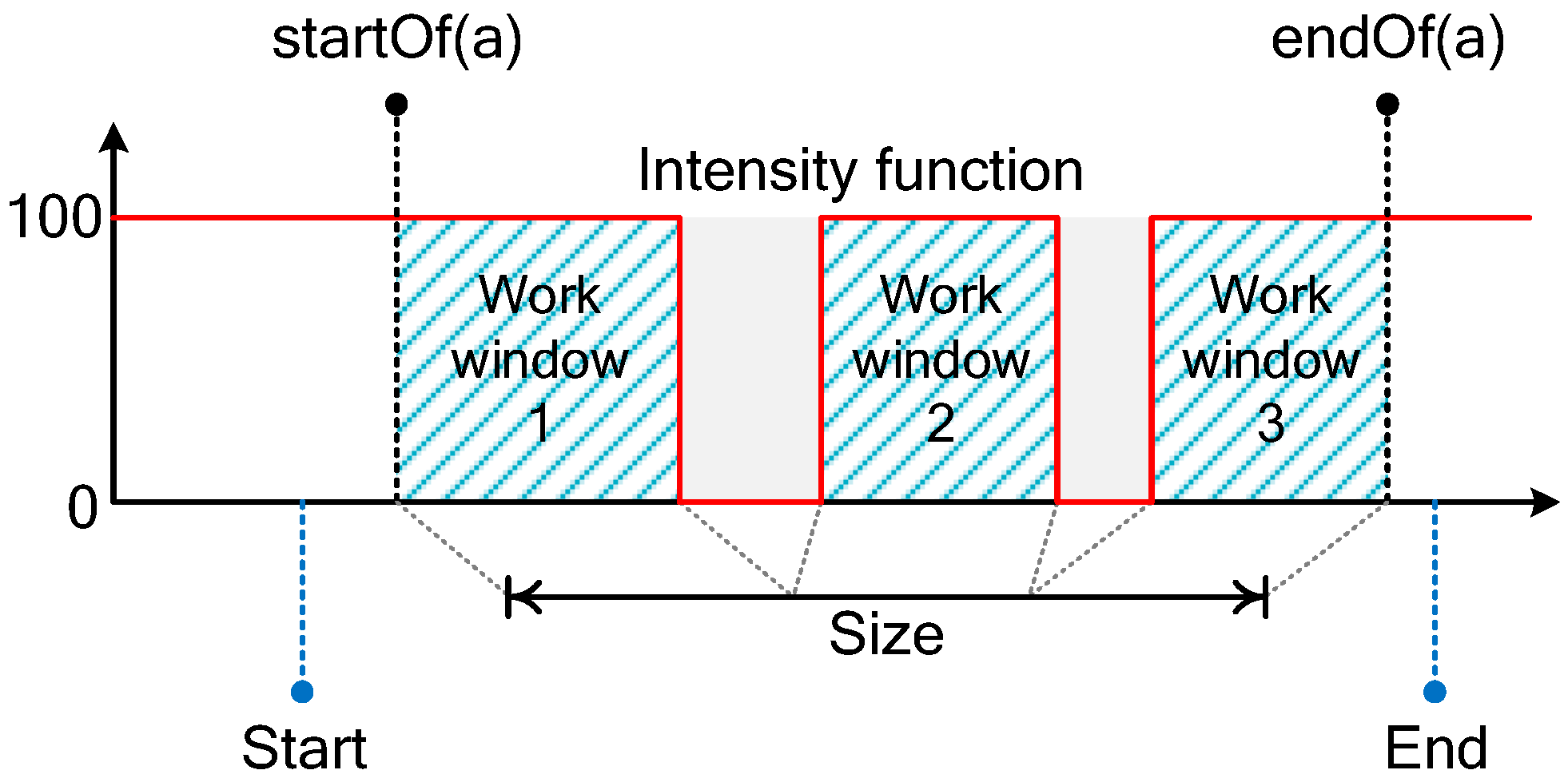
This paper utilizes the ILOG OPL language and the IBM ILOG CPLEX CP Optimizer [48] for model establishment and solving. To represent an interval of time during which an activity is performed, interval variables are used. These variables possess critical attributes such as start, end, size, and calendar, which are explained in Figure 1 and the list below.

Figure 1.
Interval variable and its attributes.
- Start and end represent the earliest start and latest finish times of an activity, respectively. For instance, if an interval variable has a start value of 2 and an end value of 14, the corresponding activity must start after time unit 2 and end before time unit 14. By default, each interval variable has a start value of zero and a given end value that is sufficiently large. Additionally, CP Optimizer’s startOf(⋅) and endOf(⋅) expressions can be used to determine the actual start and finish times of an interval variable;
- Size represents the time required to perform an activity without interruption and should be equal to the duration (processing time) of the activity at one mode in this application;
- Calendar (or intensity function) is a step function with integer values that represent the work intensity over the length of an activity. The default intensity of an activity is 100 percent and cannot exceed this value. If an activity cannot be processed during a specific time window (i.e., a rest window exists), then the intensity for that time period should be set to 0.
Interval variables allow for the expression of an activity’s duration, start and finish time, and potential work or rest windows in a single variable. Additionally, interval variables can be optional. If an optional interval variable is not present in the final solution, it will not be considered by any constraint or expression on interval variables it is involved in. Otherwise, its feasible domain will be reduced to a singleton defined by its actual start and finish time. The concept of optionality is utilized to model alternative modes and possible scheduled times for executing a given activity. CP is becoming more attractive in project scheduling literature due to its advantages [49,50].
4. Problem Description and Model Formulation
Suppose we are given a time-constrained activity network , where is the set of activities and represents the set of activity pairs. Each pair of activities indicates that activity precedes activity . The precedence relations between activities can be classified into start-to-start (SS), start-to-finish (SF), finish-to-start (FS), and finish-to-finish (FF) relations. To incorporate these precedence relations into the modeling process, the set of activity pairs is divided into four subsets , , , and , representing the sets of SS, SF, FS, and FF precedence relations, respectively.
Assuming activity 0 is the single dummy start activity and activity is the single dummy end activity, each real activity can be executed in different modes. The duration (processing time) of an activity in mode is a discrete, non-increasing function of the amount of a single non-renewable resource (money) allocated to it. The dummy activities 0 and have zero duration and zero cost. Additionally, there is a pre-specified deadline which serves as an upper bound on the project completion time.
4.1. Time Constraints
The time-constrained activity network includes three different types of time constraints: time-window, time-switch, and time-schedule constraints. As a result, activities in can be categorized as normal activities (), time-schedule activities (), time-window activities (), or time-switch activities (), where:
- A normal activity can be executed at any time after all its preceding activities are completed. The classical DTCTP assumes that all activities are normal;
- A time-schedule activity must satisfy not only the traditional precedence constraints but also its time-schedule constraint with and . Indeed, the start time of the activity can only be chosen from the set as illustrated in Figure 2a. This time constraint is frequently encountered in the construction industry and in the transportation of goods via flights, ocean liners, trains, buses, or a combination thereof, from one location to another;
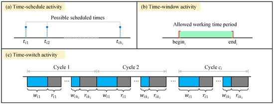 Figure 2. Graphical representation of the three types of time constraints: (a) time-schedule constraint, (b) time-window constraint, and (c) time-switch constraint.
 - A time-window activity must adhere to both precedence constraints and a time-window constraint with . The time-window constraint, as shown in Figure 2b, requires the activity to be completed within the time interval . This type of constraint is typically imposed when the activity relies on external resources (such as rented machines or equipment) that are only available during a specific time period;
- For a time-switch activity , its start time is restricted not only by precedence constraints but also by a time-switch constraint , where (or ), , is the duration of the -th work (or rest) window and is the number of pairs in a cycle. The time-switch constraint requires the activity to be active during work windows and inactive during rest windows. Figure 2c presents a graphical representation of this constraint. Work windows are depicted in blue, while rest windows are depicted in gray.
The time-switch constraint defines the work/rest pattern for the corresponding activity. Vanhoucke [44] analyzed three common work/rest patterns: day pattern, d&n pattern, and dnw pattern. The day pattern allows for activities to be executed only during daytime from Monday to Friday. The d&n pattern allows for activities to be executed during both day and night from Monday to Friday. The dnw pattern allows for activities to be executed every day and night, including weekends. According to the activity categorization above, activities with a day pattern must adhere to a time-switch constraint . Activities with a d&n pattern should meet a time-switch constraint . Additionally, activities with a dnw pattern can be treated as normal activities. The construction industry can apply these three work/rest patterns to building projects. The day pattern should be used for activities that produce noise pollution during execution, such as excavation, or for activities that are not suitable for nighttime execution, such as scaffolding erection. The d&n pattern is necessary for activities that can be executed at night, such as interior wall decoration, and when the acceleration strategy of working double shifts is adopted. If we further consider the acceleration strategy of working weekends, the activity may follow a dnw pattern. For more information on the time-constrained activity network, please refer to Guerriero and Talarico [7].
4.2. Proposed CP Model
This subsection aims to present the DTCTPTC as a CP model, which is recognized for its ability to express complex relationships and to obtain optimal or high-quality solutions within a reasonable time. The proposed CP model has several features including the following:
- (1)
- An activity may have multiple alternative modes. The duration and direct costs of the activity are known for each model;
- (2)
- Each time-switch activity can be executed in different work/rest patterns, which may affect the direct costs of the activity;
- (3)
- Time-schedule and time-window constraints are also considered. Different start times for time-scheduling activities may correspond to varying direct costs due to market price fluctuations and other factors;
- (4)
- Precedence constraints between activities can be SS, SF, FS, and FF with or without lag time;
- (5)
- The objective of the proposed CP model is to optimize the execution mode of each activity, the start times of time-schedule activities, and the work/rest patterns of time-switch activities in order to minimize the total project cost while satisfying all required constraints.
In building the CP model, the following interval variables are defined with the appropriate attribute values:
| Interval variable associated with each activity . This type of interval variable must be present in the final solution because all activities require completion; | |
| Optional interval variable with a size of representing performing normal activity in mode ; | |
| Optional interval variable with a size of , a start value of , and an end value of . If is present, time-schedule activity will be executed in mode with a start time of ; | |
| Optional interval variable with a size of , a start value of , and an end value of . This setting ensures that time-window activity will be executed within the time period , regardless of the selected mode; | |
| Optional interval variable representing performing time-switch activity in pattern with a size of . The intensity function of this variable has a value of 100 percent during all work windows in pattern and reduces to zero during all rest windows. |
The proposed CP model for the DTCTPTC is as follows:
The objective function (1) is to minimize the total cost of the project, where represents the direct cost of all normal and time-window activities, represents the direct cost of all time-schedule activities, represents the direct cost of all time-switch activities, and represents the indirect cost of the project. is calculated using Equation (2), which utilizes the CP function to determine the status of an optional interval variable in the final solution. The function returns a value of 1 if the variable is present and 0 otherwise. is calculated using Equation (3), where the parameter represents the direct cost of performing time-schedule activity in mode with a start time of . is calculated using Equation (4), where the parameter represents the direct cost of performing the time-switch activity in mode and pattern .
The indirect cost (IC) of the project includes all costs that cannot be associated with a specific activity. Most papers measure this cost as a function of the project duration, which is equal to the finish time of the single dummy end activity and can be determined using the CP function . According to the Ministry of Housing and Urban-Rural Development of the People’s Republic of China, the IC is composed of stipulated fees and enterprise management fees. Both fees can be estimated based on project direct or labor costs. For the sake of simplicity, this paper assumes that the IC is calculated as a percentage of the project’s direct cost.
Constraints (5)–(13) define the constraint system of the proposed CP model. Specifically, constraint (5) utilizes the CP global constraint to implement an exclusive alternative between the optional interval variables . If is present, then exactly one of the interval variables from the set will also be present. Furthermore, will start and end together with the chosen interval variable. Constraint (5) ensures that only one mode can be chosen for each normal activity from the set . Similarly, constraint (6) guarantees that each time-window activity is assigned to exactly one mode and executed within the given time window. Constraint (7) requires that each time-schedule activity is performed in only one mode and starts at one of the scheduled times . Constraint (8) ensures that each time-switch activity is executed in one mode and one pattern. Constraint (9) maintains the precedence constraints between activities with the SS relations. The CP constraint models the situation where activity cannot start earlier than time after the completion of activity . Constraints (10)–(12) handle the precedence constraints between activities with the SS, SF, and FF relations. Finally, constraint (13) ensures that the single dummy end activity is completed before the time unit , thus meeting the given deadline.
The advantages of using CP for model formulation can be summarized as follows. Firstly, CP is an effective method for solving combinatorial problems that are too irregular for mathematical programming [48]. The use of interval variables and their optionality makes it clear to describe alternative modes and work/rest patterns for executing a given activity. Secondly, problem description is kept separate from problem-solving, making CP models easy for practitioners to use. Meta-heuristic algorithms are commonly used to address scheduling problems in construction by searching for optimal or approximate solutions. However, their performance is highly dependent on proper implementation and parameter tuning, which can vary based on user experiences [51]. In contrast, mathematical modeling methods are based on optimization theories and maintain solution optimality. However, constructing models is typically a time-consuming and labor-intensive process [52]. Additionally, the CP model provides specialized keywords and syntax for modeling complex relationships, which allows for the easy integration of other constraints without the need to rebuild the model [49]. This improves the practicability and flexibility of CP models.
5. Model Validation
This section aims to demonstrate the application of the proposed CP model for solving the DTCTPTC through two case studies based on two literature examples. The proposed CP model was executed on a PC with an i7 CPU, 8 GB of RAM, and the Windows 10 operating system, using IBM ILOG CPLEX Studio (v12.6) for its solution.
5.1. Case Study 1
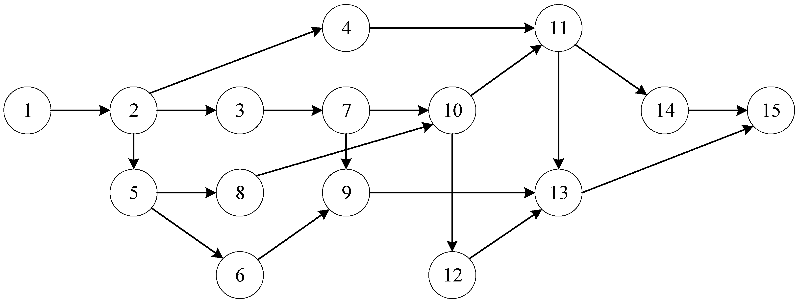
This case study considers a real project, a schedule of finishing works in a residential building. Figure 3 displays the precedence network of the project, where each pair of activities is connected by an FS precedence relation with zero lag time.
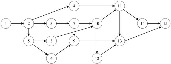
Figure 3.
Precedence network for the example project in Case Study 1.
Table 1 reports information on activities, including activity number, description, alternative modes, and possible work/rest patterns. As per the Measures of Beijing Municipality for Prevention and Control of Environmental Noise Pollution [53], any construction operation that causes environmental noise pollution is prohibited during nighttime and weekends in urban areas where noise-sensitive construction structures are concentrated. To ensure efficient execution, Activities 1 (services: plumbing, electrical, and heating services), 4 (gas piping), 12 (electrical fittings), 13 (kitchen fitted cupboards), and 14 (sanitary appliances) must be executed in a day pattern. Activities 3 and 6 are designated technological breaks, and Activity 15 is a dummy-end activity; therefore, they follow a dnw pattern. The remaining activities may choose different work/rest patterns as needed. If an activity is performed during nighttime hours, its direct cost should include the expense of night work. Additionally, if the activity is performed on weekends, the cost of the weekend should also be included.

Table 1.
Activities numbers, alternative modes, and patterns in Case Study 1.
Each real activity has two alternative modes, each with a defined duration in days and corresponding direct cost in dollars. For instance, Activity 1 can be completed in 12 days with a direct cost of USD 24,000 or in 9 days with a direct cost of USD 36,000. The indirect cost of the project is calculated as a percentage of its direct cost, with an indirect cost rate of 10 percent. The project deadline, , is set to 108 days, and the project must begin on a Monday. This project deadline is the average of the shortest project duration (SPD), 64.5 days, and the longest allowable project duration (LPD), 151.5 days. The SPD is achieved by assigning the first mode to all activities and performing Activities in a dnw pattern. The LPD can be obtained by executing all activities in the second mode and a day pattern.
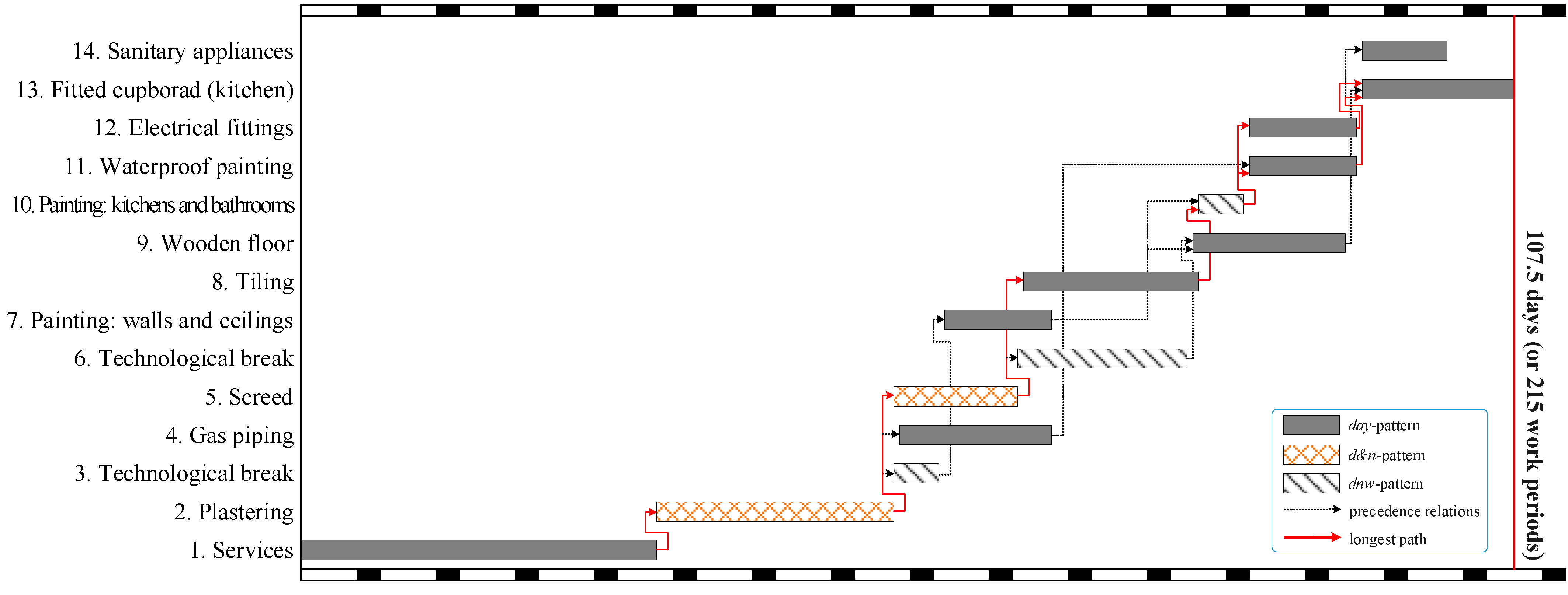
The proposed CP model can obtain the optimal solution for the project with a deadline of 108 days within 1 s. The total cost of the project is USD 80,817, which includes a direct cost of USD 73,470 and an indirect cost of USD 7347. Figure 4 shows the Gantt chart of the optimal solution. The first and last rows represent the time during which weekends are highlighted in black. The intermediate rows represent the activities numbered from 1 to 14. The figure illustrates that the project duration of the optimal solution is 107.5 days. To obtain the optimal schedule, it is clear that Activities should follow a day pattern, Activities should follow a d&n pattern, and Activities should follow a dnw pattern. Additionally, Activities should be performed in the second mode, while the remaining activities should be executed in the first mode.
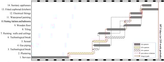
Figure 4.
Optimal schedule of the example project in Case Study 1 with a deadline of 108 days.
The author utilized the proposed CP model to create a comprehensive time–cost curve for the project. This was achieved by adjusting the deadline from 65 days to 110 days in increments of 5 days. The computational results are detailed in Table 2, in which ten non-dominated solutions are found. These results can be used as a guide for practitioners who need to implement schedule compression while adhering to time-switch constraints. The table shows that the optimal project cost is USD 82,159 with a project duration of 102.5 days if the project must be completed within 105 days. However, if the deadline is shortened to 100 days, the optimal strategy is to adjust the modes of Activities and change the work/rest pattern of Activities from day pattern to d&n pattern. As a result, the project cost increases to USD 83,116, and the corresponding project duration is 99.5 days. The computational results listed in Table 2 show that the optimal work/rest pattern of an activity may change as the deadline changes.
Table 2.
Tim-cost curve of the example project in Case study 1.
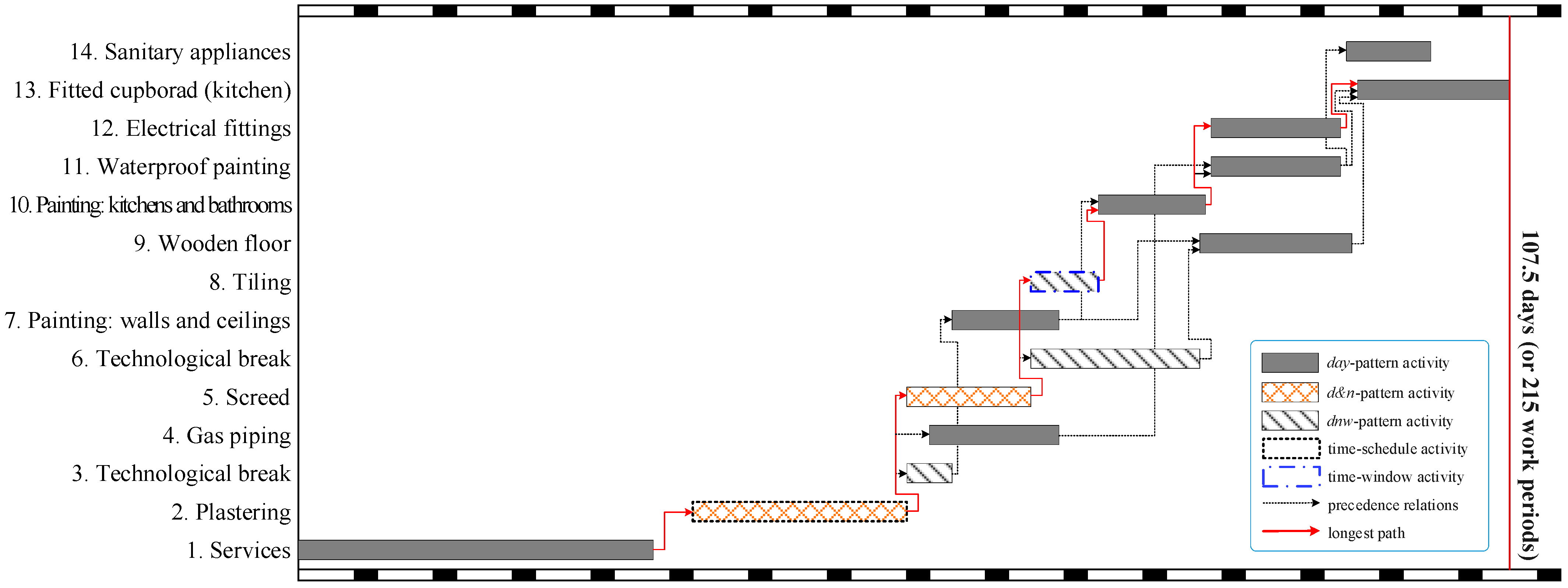
The author associates Activity 2 with an additional time-schedule constraint and Activity 8 with an additional time-window constraint . This is done in order to investigate the impact of time-schedule and time-window constraints on the schedule and validate the performance of the proposed CP model in handling different types of time constraints simultaneously. The time-schedule constraint mandates that Activity 2 must commence on Monday, Wednesday, or Friday morning of week 6. It is assumed that a different start time for Activity 2 would not affect its direct costs. Meanwhile, the time-window constraint stipulates that Activity 8 must start after day 65 and end before day 71. Figure 5 displays the Gantt chart of the optimal solution calculated by the proposed CP model with a deadline of 108 days. Compared to the schedule shown in Figure 4, the total project cost increases to USD 84,924 due to additional time constraints. The longest path, , has a length of 102 days, which is shorter than the project duration of 107.5 days. This is due to time constraints. On one hand, Activity 2 has only one predecessor (i.e., Activity 1), so its earliest possible start time is the same as the finish time of Activity 1, which is 31.5 days. On the other hand, Activity 2 is restricted by the time-schedule constraint , meaning that its start time can only be chosen from the set . Therefore, this activity cannot start immediately after its preceding activity is finished. Similar situations are also observed in Activities 12 and 13.
Figure 5.
Optimal schedule of the example project in Case Study 1 considering additional time-schedule and time-window constraints.
This case study presents an analysis of the applicability of the proposed CP model to a real-world project. In fact, the practical applications of the proposed CP model beyond this example include road maintenance and scheduling optimization of manufacturing processes. In road maintenance projects, completing all tasks within a predetermined time window is necessary to reduce traffic delays and enhance traffic safety. In the manufacturing industry, activities involving many people should follow a day pattern. The d&n pattern may be used when an activity requires only one person to control its execution occasionally. The dnw pattern may be used for activities that do not require human intervention.
5.2. Case Study 2
This case study examines a fictitious project comprising 65 activities with up to five modes to assess the efficacy of the proposed CP model in addressing large-scale issues. Table 3 displays the time–cost alternatives for each activity and the precedence relations between them; each pair of activities is linked with a zero-lag time. This project was analyzed by Sonmez and Bettemir [54] and Aminbakhsh and Sonmez [2] without considering time constraints. Therefore, we have artificially added time constraints to some of the activities. For each time-window activity, we used a loose time-window constraint to ensure the feasibility of the DTCTPTC. The time constraints for time-schedule and time-switch activities are presented in Table 4. The fictitious project comprises different time–cost alternatives, and 70% (45 out of 64) of activities have associated time constraints.
Table 3.
Types, successors, and alternative modes of all activities in Case Study 2.
Table 4.
Time constraints for time-schedule and time-switch activities in Case Study 2.
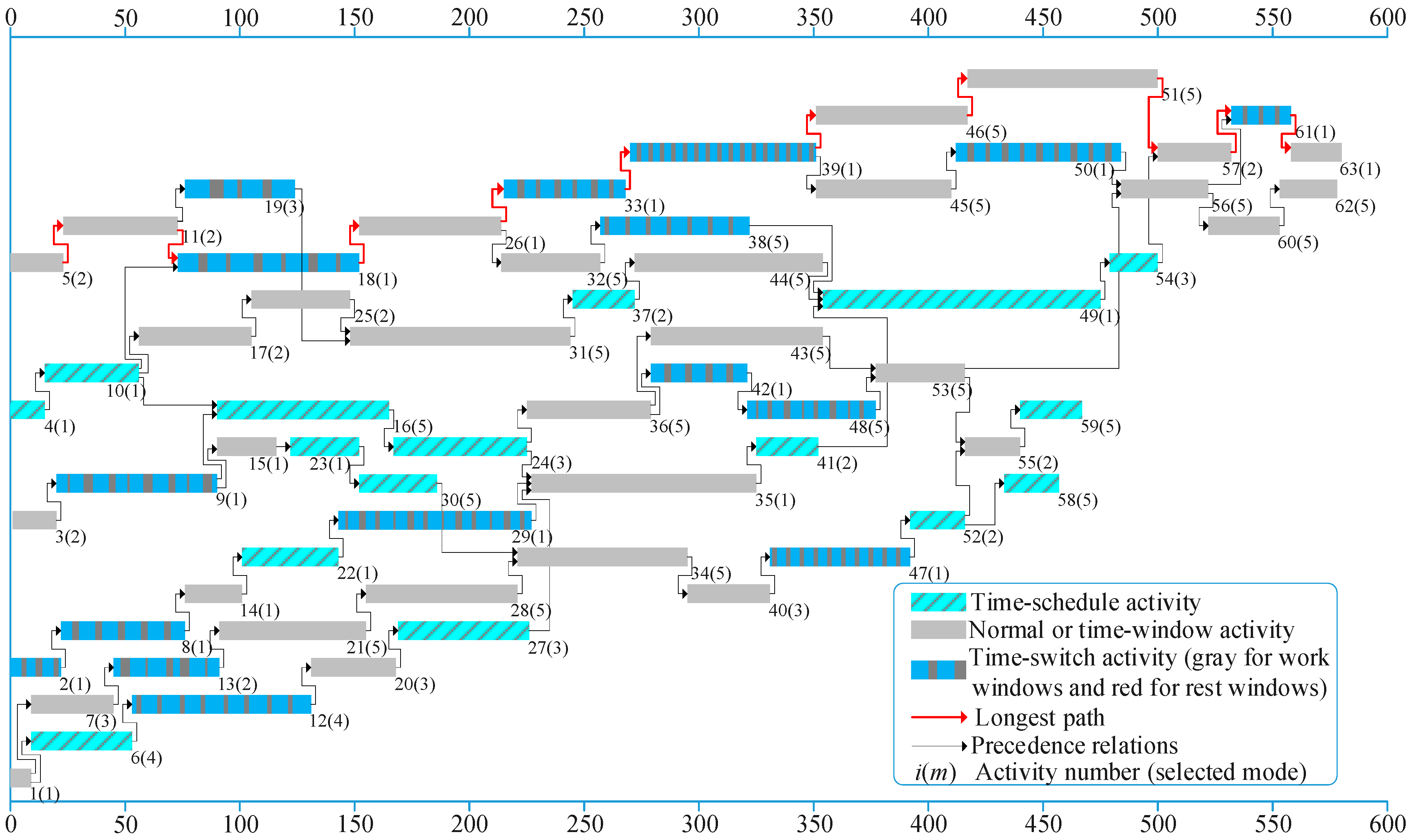
Figure 6 shows the optimal schedule for the fictitious project with a deadline of 580 days, obtained by the proposed CP model within 1 s. As in case study 1, we observed that not every activity in a time-constrained network can start as soon as all of its predecessors are finished due to the presence of time constraints. For instance, although time-schedule activity 58 has only one preceding activity 52 that can end before day 416, it cannot begin before day 433 due to the time-schedule constraint . Additionally, the length of the critical path in a time-constrained activity network is likely to exceed the total working time of all activities on the path if there are critical activities with time constraints. To be specific, the critical path of the schedule shown in Figure 6 is with a length of 580 days. However, the total working time of all critical activities on the path is only 506 days.
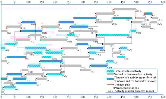
Figure 6.
Optimal schedule of the example project in Case Study 2 with a deadline of 580 days.
6. Discussion
The analysis of the two case studies presented in the previous section indicates that time-constrained networks have distinct characteristics compared to traditional networks. To enhance the practicability of scheduling optimization models, it is vital to integrate time constraints. Failure to take this into account may result in an inappropriate project schedule and management, leading to an inefficient or even infeasible solution. As previously stated in the literature review, only the algorithms proposed by Vanhoucke et al. [43] and Vanhoucke [44] are capable of handling the DTCTPTC. However, these algorithms assume that there is only one work/rest pattern for each activity, which undoubtedly restricts the application of the algorithm and the quality of the solution. To illustrate, in Case Study 1, assuming that all activities adhere to a day pattern, the total cost estimated by the algorithms of Vanhoucke et al. [43] and Vanhoucke [44] is USD 98,725. The corresponding schedule was obtained by performing Activities 1, 2, 5, 8, 10, and 13 using the first mode and executing the remaining activities by the second model. When compared to the calculation results of the proposed CP model (Figure 4), this schedule leads to an increase in the total cost by 22.16%. A further limitation of previous algorithms is the assumption that only time-switch constraints exist in time-constrained networks. Consequently, these algorithms are unable to accommodate DTCTPs with time-window and time-schedule constraints in the same manner as the proposed CP model.
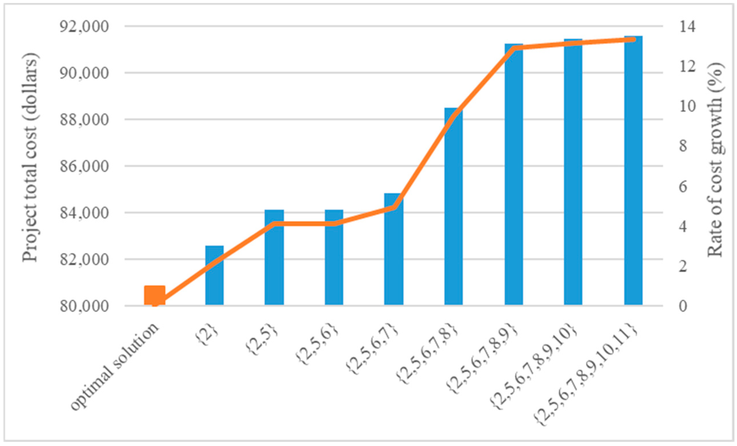
One of the key features of the proposed CP model is the classification of activities into distinct categories, including normal activities, time-window activities, time-scheduling activities, and time-switch activities. If all activities are classified as normal activities, the proposed model will essentially become the traditional DTCTP model. The real-life project in Case Study 1 is comprised of 15 time-switch activities. Three of these activities follow a dnw pattern, five must follow a day pattern, and the remaining seven (2, 5, 7, 8, 9, 10, and 11) have three alternative work/rest patterns: day pattern, d&n pattern, and dnw pattern. The dnw pattern allows for activities to be executed every day and night, including weekends. Therefore, activities with a dnw pattern can be treated as normal activities. A sensitivity analysis is now conducted, whereby the work/rest pattern of activities 2, 5, 7, 8, 9, 10, and 11 are progressively replaced with the dnw pattern, and the resulting change in the total project cost is observed. Figure 7 illustrates the results of the sensitivity analysis. As the number of activities adopting the dnw pattern increases, the total project cost shows a significant increase, reaching a maximum of 13.31%. This result suggests that the work/rest pattern of activities is an important optimization element and that there is a need to develop methods for solving the DTCTPTC similar to the proposed CP model.
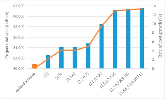
Figure 7.
Sensitivity analysis of the set of activities with a work/rest pattern set to the dnw pattern.
The potential limitations of the proposed CP model can be summarized as follows. First, the model may produce schedules in which multiple activities are scheduled to occur simultaneously, increasing site congestion, accident risks and worker fatigue. To compensate this limitation, an effective way is to integrate the proposed CP model with resource constraints that limit the number of activities that are performed simultaneously. This idea can be easily implemented using the CP function , which returns an expression equal to everywhere between the start and the end of the interval variable , and equal to 0 outside the interval. Consequently, the resource distribution can be determined by the algebraic sum of the pulse functions of . Another alternative is to consider location and congestion so that activities are scheduled to avoid workspace interference. The reader interested in this aspect can refer to the paper by Tao et al. [55]. Second, to simplify the model, this paper assumes that the productivity of an activity during the day shift is the same as during the night shift. This assumption may not be true in some situations. However, this limitation can be easily overcome by resetting the intensity function of the interval associated with the activity.
7. Conclusions
During the planning phase of a construction project, one of the primary tasks is to implement a time–cost tradeoff analysis to determine an efficient schedule. This paper presented a CP model for solving the DTCTPTC. The objective is to optimize the execution mode of each activity, the start times of time-schedule activities, and the work/rest patterns of time-switch activities in order to minimize the total cost of the project while satisfying all required constraints. To illustrate the effectiveness of the proposed CP model, two projects from the literature were examined. This enhances the practicality of the proposed model.
The proposed CP model adds three types of time constraints to the scheduling process, which can assist planners in modelling time-window, time-schedule, and time-switch activities. However, these constraints also pose significant challenges to the design and scheduling of a project when compared to traditional DTCTP models. During the planning stage, the project management team must provide an accurate description of time-window and time-schedule constraints for related activities, and determine the available work/rest patterns for each activity. Throughout the construction phase, a series of schedule control measures must be implemented to ensure that all activities, particularly those with time constraints, are executed as planned. If available, the schedule obtained by the proposed model can be used in practice.
The contributions of this study are twofold. Firstly, it establishes a new DTCTP scheduling framework that integrates three different types of time constraints, making it more valuable for practical applications. The framework assists project managers in balancing the project completion time and cost, taking into account precedence constraints, time constraints and a deadline constraint. Secondly, an efficient CP model is developed using interval variables and global constraints extracted from IBM’s CP Optimizer. This model enables project managers to acquire high-quality solutions within a relatively short timeframe. Literature has conducted several studies to determine the critical path (longest path) and analyze the float of each activity in a time-constrained activity network. The combination of these research works and the proposed CP model improves project management by enhancing resource utilization and progress control.
Construction projects frequently encounter various uncertainties during their execution. Even if planned schedules are optimal, their implementation may be affected by these uncertainties, resulting in project delays, cost overruns, or both. Consequently, an intriguing avenue for future research would be to analyze the DTCTPTC in an uncertain environment. Common uncertainty approaches include stochastic, fuzzy, and robust optimization. In stochastic optimization, the parameters of a project are assumed to be probabilistic, with their probability distribution functions derived from historical data. However, in some cases, the lack of historical data may prevent the determination of the probability distribution functions of the project parameters. Currently, the use of fuzzy optimization, which employs membership functions based on possibility theory as a replacement for probability distributions, is preferable. In contrast, robust optimization is designed to construct a stable project schedule capable of minimizing the impact of unexpected events on the main performance criteria. In this approach, all parameters are generally deterministic.
Author Contributions
Conceptualization, Y.L. and X.Z.; methodology, D.L. and X.Z.; software, D.L. and Y.R.; validation, Y.R., P.S. and X.Z.; formal analysis, X.Z.; investigation, Y.L. and D.L.; resources, Y.R.; data curation, P.S.; writing—original draft preparation, Y.L. and D.L.; writing—review and editing, X.Z.; visualization, Y.R.; supervision, P.S.; project administration, Y.L. and X.Z.; funding acquisition, X.Z. All authors have read and agreed to the published version of the manuscript.
Funding
This work was funded by the National Natural Science Foundation of China grant number 72171081, the Natural Science Foundation of Hebei Province of China grant number G2022502001, and the Fundamental Research Funds for the Central Universities grant number 2023MS153. The authors are also grateful to the anonymous reviewer and editor for a careful scrutiny of details and for comments that helped improve this manuscript.
Data Availability Statement
The original contributions presented in the study are included in the article, further inquiries can be directed to the corresponding author.
Conflicts of Interest
Authors Yang Liu and Dawei Liu were employed by the company State Grid East Inner Mongolia Electric Power Supply Co., Ltd. Authors Yanzhao Rong and Penghui Song were employed by the company China Railway Construction Engineering Group. The remaining authors declare that the research was conducted in the absence of any commercial or financial relationships that could be construed as a potential conflict of interest.
References
- ElSahly, O.M.; Ahmed, S.; Abdelfatah, A. Systematic review of the time-cost optimization models in construction management. Sustainability 2023, 15, 5578. [Google Scholar] [CrossRef]
- Aminbakhsh, S.; Sonmez, R. Discrete particle swarm optimization method for the large-scale discrete time–cost trade-off problem. Expert Syst. Appl. 2016, 51, 177–185. [Google Scholar] [CrossRef]
- Tareghian, H.R.; Taheri, S.H. On the discrete time, cost and quality trade-off problem. Appl. Math. Comput. 2006, 181, 1305–1312. [Google Scholar] [CrossRef]
- De, P.; Dunne, E.J.; Ghosh, J.B.; Wells, C.E. The discrete time-cost tradeoff problem revisited. Eur. J. Oper. Res. 1995, 81, 225–238. [Google Scholar] [CrossRef]
- Chen, Y.L.; Rinks, D.; Tang, K. Critical path in an activity network with time constraints. Eur. J. Oper. Res. 1997, 100, 122–133. [Google Scholar] [CrossRef]
- Yang, H.H.; Chen, Y.L. Finding the critical path in an activity network with time-switch constraints. Eur. J. Oper. Res. 2000, 120, 603–613. [Google Scholar] [CrossRef]
- Guerriero, F.; Talarico, L. A solution approach to find the critical path in a time-constrained activity network. Comput. Oper. Res. 2010, 37, 1557–1569. [Google Scholar] [CrossRef]
- Gedik, R.; Kirac, E.; Milburn, A.B.; Rainwater, C. A constraint programming approach for the team orienteering problem with time windows. Comput. Ind. Eng. 2017, 107, 178–195. [Google Scholar] [CrossRef]
- Peng, W.L.; Wang, C.G. A multi-mode resource-constrained discrete time–cost tradeoff problem and its genetic algorithm based solution. Int. J. Proj. Manag. 2009, 27, 600–609. [Google Scholar]
- Hafızoğlu, A.B.; Azizoğlu, M. Linear programming based approaches for the discrete time/cost trade-off problem in project networks. J. Oper. Res. Soc. 2010, 61, 676–685. [Google Scholar] [CrossRef]
- Klanšek, U.; Pšunder, M. MINLP optimization model for the nonlinear discrete time–cost trade-off problem. Adv. Eng. Softw. 2012, 48, 6–16. [Google Scholar] [CrossRef]
- Szmerekovsky, J.G.; Venkateshan, P. An integer programming formulation for the project scheduling problem with irregular time–cost tradeoffs. Comput. Oper. Res. 2012, 39, 1402–1410. [Google Scholar] [CrossRef]
- Choi, B.C.; Kang, C. A linear time–cost tradeoff problem with multiple milestones under a comb graph. J. Comb. Optim. 2019, 38, 341–361. [Google Scholar] [CrossRef]
- Aouam, T.; Vanhoucke, M. An agency perspective for multi-mode project scheduling with time/cost trade-offs. Comput. Oper. Res. 2019, 105, 167–186. [Google Scholar] [CrossRef]
- Eynde, R.V.; Vanhoucke, M. A reduction tree approach for the discrete time/cost trade-off problem. Comput. Oper. Res. 2022, 143, 105750. [Google Scholar] [CrossRef]
- Nasiri, S.; Lu, M. Streamlined project time-cost tradeoff optimization methodology: Algorithm, automation, and application. Autom. Constr. 2022, 133, 104002. [Google Scholar] [CrossRef]
- Wang, J.; Han, C.J.; Li, X.H. Modified streamlined optimization algorithm for time-cost tradeoff problems of complex large-scale construction projects. J. Constr. Eng. Manag. 2023, 149, 04023022. [Google Scholar] [CrossRef]
- Daboul, S.; Held, S.; Vygen, J. Approximating the discrete time-cost tradeoff problem with bounded depth. Math. Program. 2023, 197, 529–547. [Google Scholar] [CrossRef]
- Alavipour, S.R.; Arditi, D. Time-cost tradeoff analysis with minimized project financing cost. Autom. Constr. 2019, 98, 110–121. [Google Scholar] [CrossRef]
- Togan, V.; Eirgas, M.A. Time-cost tradeoff optimization with a new initial population approach. Tek. Dergi 2019, 30, 9561–9580. [Google Scholar] [CrossRef]
- Banihashemi, S.A.; Khalilzadeh, M.; Antucheviciene, J.; Šaparauskas, J. Trading off Time–Cost–Quality in Construction Project Scheduling Problems with Fuzzy SWARA–TOPSIS Approach. Buildings 2021, 11, 387. [Google Scholar] [CrossRef]
- Gupta, R.; Trivedi, M.K. AEHO: Apriori-Based Optimized Model for Building Construction to Time-Cost Tradeoff Modeling. IEEE Access 2022, 10, 103852–103871. [Google Scholar] [CrossRef]
- Bettemir, Ö.H.; Birgonul, M.T. Solution of discrete time–cost trade-off problem with adaptive search domain. Eng. Constr. Archit. Manag. 2023. ahead-of-print. [Google Scholar]
- Son, P.V.H.; Nguyen Dang, N.T. Solving large-scale discrete time–cost trade-off problem using hybrid multi-verse optimizer model. Sci. Rep. 2023, 13, 1987. [Google Scholar] [CrossRef] [PubMed]
- El-Rayes, K.; Kandil, A. Time-cost-quality trade-off analysis for highway construction. J. Constr. Eng. Manag. 2005, 131, 477–486. [Google Scholar] [CrossRef]
- Cheng, M.Y.; Tran, D.H. Opposition-based multiple-objective differential evolution to solve the time–cost–environment impact trade-off problem in construction projects. J. Comput. Civ. Eng. 2015, 29, 04014074. [Google Scholar] [CrossRef]
- Mohammadipour, F.; Sadjadi, S.J. Project cost–quality–risk tradeoff analysis in a time-constrained problem. Comput. Ind. Eng. 2016, 95, 111–121. [Google Scholar] [CrossRef]
- Hariga, M.; Shamayleh, A.; El-Wehedi, F. Integrated time–cost tradeoff and resources leveling problems with allowed activity splitting. Int. Trans. Oper. Res. 2019, 26, 80–99. [Google Scholar] [CrossRef]
- Heravi, G.; Moridi, S. Resource-Constrained Time-Cost Tradeoff for Repetitive Construction Projects. KSCE J. Civ. Eng. 2019, 29, 3265–3274. [Google Scholar] [CrossRef]
- Banihashemi, S.A.; Khalilzadeh, M.; Shahraki, A.; Malkhalifeh, M.R.; Ahmadizadeh, S.S.R. Optimization of environmental impacts of construction projects: A time–cost–quality trade-off approach. Int. J. Environ. Sci. Technol. 2021, 18, 631–646. [Google Scholar] [CrossRef]
- Chen, L.W.; Zhang, J.W.; Peng, W.L. Research on the hierarchical discrete time-cost tradeoff problem for program. J. Constr. Eng. Manag. 2022, 148, 04022039. [Google Scholar] [CrossRef]
- Yazdani, M.; Aouam, T.; Vanhoucke, M. An exact decomposition technique for the deadline-constrained discrete time/cost trade-off problem with discounted cash flows. Comput. Oper. Res. 2024, 163, 106491. [Google Scholar] [CrossRef]
- Hosseinzadch, F.; Paryzad, B.; Najafi, E. Fuzzy combinatorial optimization in four-dimensional tradeoff problem of cost-time-quality-risk in one dimension and in the second dimension of risk context in ambiguous mode. Eng. Comput. 2020, 37, 1967–1991. [Google Scholar] [CrossRef]
- Mahdiraji, H.A.; Sedigh, M.; Hajiagha, S.H.R.; Garza-Reyes, J.A.; Jafari-Sadeghi, V.; Dana, L.P. A novel time, cost, quality and risk tradeoff model with a knowledge-based hesitant fuzzy information: An R&D project application. Technol. Forecast. Soc. Chang. 2021, 172, 121068. [Google Scholar]
- Lotfi, R.; Karagar, B.; Amra, M. Resource-constrained time-cost-quality-energy-environment tradeoff problem by considering blockchain technology, risk and robustness: A case study of healthcare project. Environ. Sci. Pollut. Res. 2022, 29, 63560–63576. [Google Scholar] [CrossRef] [PubMed]
- Abdel-Basset, M.; Ali, M.; Atef, A. Uncertainty assessments of linear time-cost tradeoffs using neutrosophic set. Comput. Ind. Eng. 2020, 141, 106286. [Google Scholar] [CrossRef]
- Godinho, P.; Costa, J.P. A stochastic model and algorithms for determining efficient time-cost tradeoffs for a project activity. Oper. Res. 2020, 20, 319–348. [Google Scholar] [CrossRef]
- Tao, L.Y.; Su, X.B.; Javed, S.A. Time-cost trade-off model in GERT-type network with characteristic function for project management. Comput. Ind. Eng. 2022, 169, 108222. [Google Scholar] [CrossRef]
- Lotfi, R.; Yadegari, Z.; Hosseini, S.H.; Khameneh, A.; Tirkolaee, E.; Weber, G. A robust time-cost-quality-energy-environment tradeoff with resource-constrained in project management: A case study for a bridge construction project. J. Ind. Manag. Optim. 2022, 18, 375–396. [Google Scholar] [CrossRef]
- Li, X.; He, Z.W.; Wang, N.M.; Vanhoucke, M. Multimode time-cost-robustness tradeoff project scheduling problem under uncertainty. J. Comb. Optim. 2022, 43, 1173–1202. [Google Scholar] [CrossRef]
- Mahdavi-Roshan, P.; Mousavi, S.M. A new interval-valued fuzzy multi-objective approach for project time–cost–quality trade-off problem with activity crashing and overlapping under uncertainty. Kybernetes 2023, 52, 4731–4759. [Google Scholar] [CrossRef]
- Kostrzewa-Demczuk, P. Construction schedule versus various constraints and risks. Appl. Sci. 2024, 14, 196. [Google Scholar] [CrossRef]
- Vanhoucke, M.; Demeulemeester, E.; Herroelen, W. Discrete time/cost trade-offs in project scheduling with time-switch constraints. J. Oper. Res. Soc. 2002, 53, 741–751. [Google Scholar] [CrossRef]
- Vanhoucke, M. New computational results for the discrete time/cost trade-off problem with time-switch constraints. Eur. J. Oper. Res. 2005, 165, 359–374. [Google Scholar] [CrossRef]
- Frühwirth, T.; Abdennadher, S. Essentials of Constraint Programming; Springer Science & Business Media: Berlin/Heidelberg, Germany, 2003. [Google Scholar]
- Apt, K. Principles of Constraint Programming; Cambridge University Press: Cambridge, UK, 2003. [Google Scholar]
- Rossi, F.; Van Beek, P.; Walsh, T. Handbook of Constraint Programming; Elsevier: Amsterdam, The Netherlands, 2006. [Google Scholar]
- IBM. IBM ILOG CPLEX Optimization Studio OPL Language Reference Manual V12.6; IBM: Armonk, NY, USA, 2015. [Google Scholar]
- Tang, Y.; Liu, R.; Wang, F.; Sun, Q.; Kandil, A.A. Scheduling optimization of linear schedule with constraint programming. Comput.-Aided Civ. Infrastruct. Eng. 2018, 33, 124–151. [Google Scholar] [CrossRef]
- Zou, X.; Rong, Z. Resource-constrained repetitive project scheduling with soft logic. Eng. Constr. Archit. Manag. 2024. ahead-of-print. [Google Scholar]
- Liu, S.S.; Wang, C.J. Optimization model for resource assignment problems of linear construction projects. Autom. Constr. 2007, 16, 460–473. [Google Scholar] [CrossRef]
- Liu, S.S.; Wang, C.J. Optimizing linear project scheduling with multi-skilled crews. Autom. Constr. 2012, 24, 16–23. [Google Scholar] [CrossRef]
- Beijing Municipal Government. Measures of Beijing Municipality for Prevention and Control of Environmental Noise Pollution. Available online: http://www.beijing.gov.cn/zhengce/zhengcefagui/201905/t20190522_56690.html (accessed on 1 July 2024).
- Sonmez, R.; Bettemir, Ö.H. A hybrid genetic algorithm for the discrete time-cost trade-off problem. Expert Syst. Appl. 2012, 39, 11428–11434. [Google Scholar] [CrossRef]
- Tao, S.; Wu, C.Z.; Sheng, Z.H.; Wang, X.Y. Space-time repetitive project scheduling considering location and congestion. J. Comput. Civ. Eng. 2018, 32, 04018017. [Google Scholar] [CrossRef]

Disclaimer/Publisher’s Note: The statements, opinions and data contained in all publications are solely those of the individual author(s) and contributor(s) and not of MDPI and/or the editor(s). MDPI and/or the editor(s) disclaim responsibility for any injury to people or property resulting from any ideas, methods, instructions or products referred to in the content. |
© 2024 by the authors. Licensee MDPI, Basel, Switzerland. This article is an open access article distributed under the terms and conditions of the Creative Commons Attribution (CC BY) license (https://creativecommons.org/licenses/by/4.0/).