Article

A Prediction Model for Soil–Water Characteristic Curve Based on Machine Learning Considering Multiple Factors

1
Department of Civil Engineering, University of Science and Technology Beijing, Beijing 100083, China
2
College of Smart Manufacturing and Intelligent Transportation, Suzhou City University, Suzhou 215104, China
3
National Center for Materials Service Safety, University of Science and Technology Beijing, Beijing 100083, China
*
Author to whom correspondence should be addressed.
Buildings 2024, 14(7), 2087; https://doi.org/10.3390/buildings14072087
Submission received: 6 June 2024 / Revised: 2 July 2024 / Accepted: 5 July 2024 / Published: 8 July 2024
(This article belongs to the Special Issue Research on Intelligent Geotechnical Engineering)

Abstract

:
Aiming at the problem of long soil–water characteristic curve (SWCC) testing times and the difficulty of prediction accuracy in complex environments, this paper establishes a SWCC prediction model based on a neural network machine learning algorithm which can take into account the influence of multiple factors such as temperature, deformation, and salinity. The input layer of the model can reflect the physical properties of the soil and the influence of the external environment, while the suction is taken as an input variable, which in turn can directly obtain the water content under the corresponding conditions. The predictive ability of the model is verified by comparing and analyzing the predicted results of the SWCC under different temperature, void ratio, and salinity conditions with the experimental results. The research in this paper provides a new method for predicting the SWCC considering multiple factors, and the prediction accuracy of the model is related to the amount of experimental data.

1. Introduction

The soil–water characteristic curve (SWCC) is a quantitative relationship that describes the potential energy (matric suction) and water content (volumetric moisture content, saturation, mass moisture content) of soil [1]. It can reflect the microscopic connections between different phases in unsaturated soil and is used to study the permeability, deformation, strength, and multi-field coupling behavior of unsaturated soil [2,3,4]. It is essential in the research of unsaturated soil theory. Some scholars provide SWCC models by fitting experimental data, such as the well-known FX model [5] and VG model [6]. However, the parameters in the model are not fixed and vary with changes in the external environment, which results in a set of model parameters only reflecting the soil–water characteristics under certain specific conditions and which are unable to achieve the predictive function of the model for different environments [7,8].
With the development of modern society, the environment in which engineering construction takes place is becoming increasingly complex, involving the coupling problem in multiple fields such as seepage, deformation, temperature, and chemical, which poses severe challenges to geotechnical engineering (geological storage of nuclear waste [9], design of landfill sites [10], engineering construction on salinized soil [11], remediation of contaminated soil [12]). This also puts high demands on SWCC models that can reflect complex environments. At present, in the research on SWCC models, although some scholars have considered the effects of deformation, temperature, salinity, etc., these studies generally only focus on the influence of a single factor and are limited to a small range of changes, and there are few studies that consider the combined influence of two or three factors [13,14]. What is worse, obtaining a soil–water characteristic curve within the full suction range requires a large amount of experimental measurement data, and the entire experimental process requires a long time [15].
With the widespread application of machine learning, a new approach has been provided for predicting the SWCC in complex environments. By learning from a large amount of existing experimental data, the evolution law of matric suction and water content of unsaturated soil under different conditions can be predicted. Therefore, some scholars have conducted research on the prediction of the SWCC using machine learning methods [15,16,17]. For example, Li and Vanapalli [17] used the grain-size distribution curve as input information and established a SWCC prediction model using artificial neural networks (ANNs) and multiple adaptive regression splines (MARSs) as analysis methods. Pham et al. [15] utilized the advantages of multiple machine learning models and the unsaturated soil database (UNSODA) to develop a new pedotransfer function to estimate the SWCC. These methods provide new solutions for the prediction of the SWCC, but there are still some limitations, such as the difficulty in considering the influence of external environments such as stress history, temperature, deformation, salinity, etc.
Currently, there are two main problems with the research on soil–water characterization. On the one hand, it is due to the long SWCC testing period in the full suction range, which leads to insufficient test data at present. On the other hand, most of the studies on SWCC modeling are based on the fitting of empirical formulas, and there are also some studies on simple prediction by machine learning methods, but it is difficult to predict the SWCC directly. Furthermore, these two problems are also more prominent under the condition of considering the influence of multiple factors. If the existing valuable data can be utilized to better predict the soil–water characteristic under the influence of different environmental factors, it can not only compensate for the problem of limited data due to the long testing period and multiple influencing factors, but can also provide a strong support for the research on a multi-field coupling model for unsaturated soil.
This paper adopts a neural network method that can learn from a large amount of existing experimental data and on-site measurement data to more accurately calculate soil–water characteristics under different conditions [14,15,16,17,18,19,20,21,22,23,24,25,26,27,28,29,30,31,32,33,34,35,36,37,38,39,40,41,42,43,44,45]. The input feature quantities can cover factors such as soil particle size, density, plasticity index, environmental temperature, matrix suction, void ratio, salinity, and stress history, and can directly use water content as the predicted output value. The hidden layer includes a certain number of neurons, neural network parameters such as weights and biases, and is optimized using gradient-based algorithms. In addition, further learning can be achieved by increasing the sample size in different regions, thereby improving the adaptability to soil samples under different conditions and having better generalization ability.

2. Construction of Neural Network Prediction Model

2.1. Data Collection and Processing

The physical properties of soil, initial conditions, and external environment are the three main factors affecting the shape of SWCC. Selected physical properties such as soil particle size d10/d30/d60 (types of particle sizes; the mass of soil particles smaller than these sizes account for 10%, 30%, and 60% of the total mass, respectively) and plasticity index Ip are the first components of the input layer. The initial water content w0 and void ratio e0 are the second components of the input layer. The external environmental temperature T and salinity C serve as the third components of the input layer. Simultaneously considering the volumetric water content under different suction conditions, the matrix suction s is also taken as the input value.
Considering that there are almost no experiments in the existing literature that simultaneously consider the effects of deformation, temperature, and salinity on the SWCC, three datasets were established. Dataset 1 considers the effects of salinity and deformation, dataset 2 considers the effects of temperature and deformation, and both datasets consider the other influencing factors mentioned above. The neural network input layers trained on both datasets contain eight variables. Dataset 3 combines datasets 1 and 2 together, with dataset 1 having a data temperature of 25 °C at room temperature and dataset 2 having a data salinity of 0 mol/L. Therefore, the input layer of the neural network trained in dataset 3 contains nine variables.
Before using neural networks for prediction, well-processed datasets can significantly improve the prediction accuracy of neural networks. Optimizing the database not only focuses on the quantity of data samples, but also on their quality, and removing abnormal data can help reduce the workload of optimizing neural network parameters. This paper collected experimental data from the literature on the SWCC published in recent decades, and these have been listed in the References section [14,15,16,17,18,19,20,21,22,23,24,25,26,27,28,29,30,31,32,33,34,35,36,37,38,39,40,41,42,43,44,45]; after sorting, 1000 sets of effective data were selected. The SWCC test types include tests on different types of soil, as well as tests affected by void ratios, temperature, and salinity. The experimental results are obtained through strict testing, which can ensure the accuracy of the results. The specific experimental details are documented in the cited literature and are not elaborated on here. Due to the different methods used in the various experiments, such as the pressure plate method, steam equilibrium method, etc., the range of eigenvalues such as matrix suction varies greatly among the different experiments. The maximum/minimum normalization method is used to normalize the input eigenvalues in the same proportion, and the processed value range is 0–1. At the same time, abnormal data are deleted. Finally, there are 400 sets of data in dataset 1, 400 sets of data in dataset 2, and 800 sets of data in dataset 3.

2.2. Model Building

To prevent overfitting of the neural network, Bayesian regularization is adopted to improve the universality of the model. The neural network for optimizing parameters using a Bayesian algorithm, also known as the Bayesian regularization neural network (BRNN), has a longer training time compared to other algorithms, but the prediction accuracy can be improved. It is worth noting that BRNN does not require a validation set, meaning the entire data are randomly divided into two parts, with 80% of the data used for model training and 20% for model testing. When the given training result standard is reached, the training process stops.
After normalizing the dataset, it is randomly divided into training and testing sets to ensure the representativeness of the entire dataset. Among them, there are 320 sets of data in the training set and 80 sets of data in the testing set. As shown in Figure 1, the BRNN neural network model has nine input variables, namely particle size d10/d30/d60, plasticity index, initial moisture content, void ratio, temperature, salinity, and matrix suction. It is worth mentioning that when only considering two factors among temperature, salinity, and deformation, there are only eight input variables. The output layer has one node, which is the volume moisture content, and the hidden layer has 25 neurons.
The transfer function from the input layer to the hidden layer is the Purelin function y = x, and the activation function of the hidden layer is the tansig function f ( x ) = 2 1 + e 2 x 1 . If the expected output is not obtained at the output layer, it enters the backpropagation stage. The loss function used is the mean square error loss function as follows
l o s s = y w x + b 2
L 2 n o r m = y w x + b 2
l o s s = n o r m y w x + b 2
Return the error signal along the original connection path and minimize the error signal by modifying the weights of each neuron. This process is optimized using the stochastic gradient descent method. In addition, the model adopts a Bayesian regularization algorithm to prevent overfitting problems.

2.3. Neural Network Training

Use two statistical measures, mean square error (MSE) and fitting degree (R), to evaluate the predictive ability of the neural model, which is the difference between the predicted target value and the true target value. The smaller the MSE value while ensuring that the R value is closer to 1, the stronger the predictive ability of the model. The MSE and R statistics are also influenced by the number of neurons in the hidden layer of the neural network. Increasing the number of neurons can enhance the computational power of the model and improve its predictive performance. However, it is not the case that the more neurons the better, as an increase in the number of neurons can lead to longer training times. For example, during the training process, when the number of hidden layer neurons increased from 10 to 25, the MSE value decreased by 12.56, and the R value increased by 0.13; when the number of hidden layer neurons increased from 25 to 50, the MSE value increased by 9.661, and the R value decreased by 0.082. By continuously adjusting the number of hidden layer nodes in the model, the number of hidden layer neurons is determined to be 25, and the model is optimized until the best predictive model is obtained.
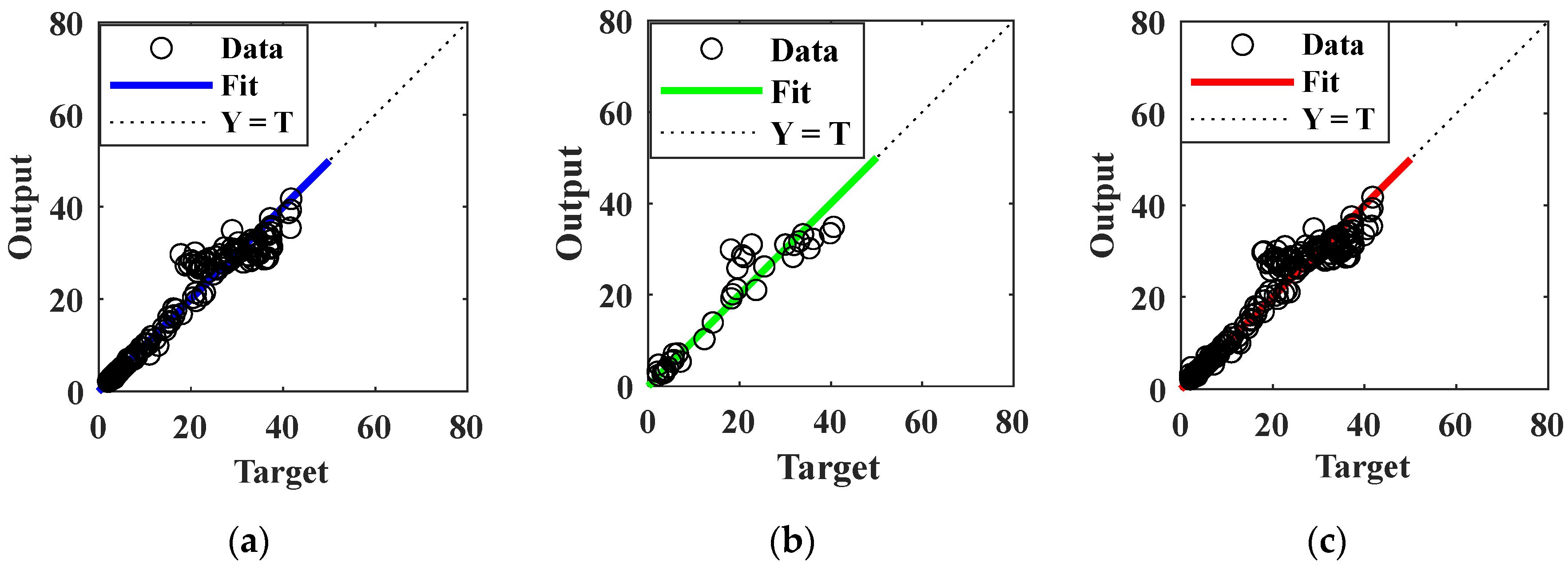
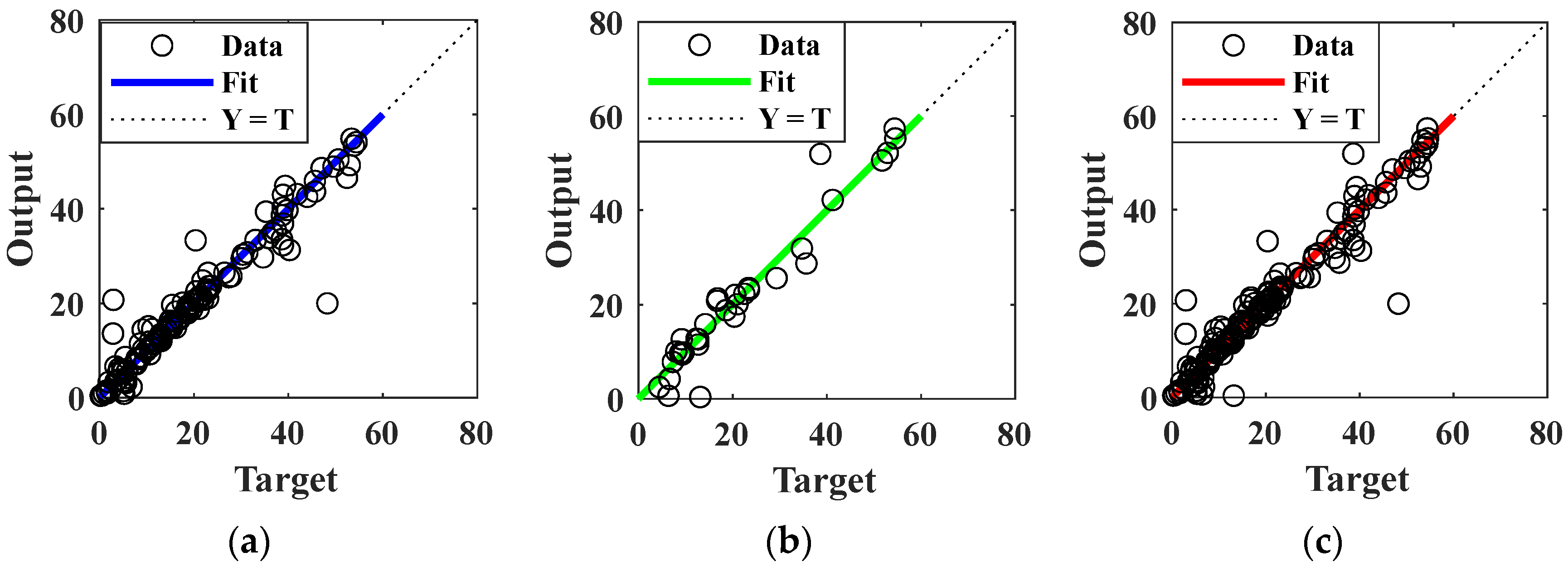
The SWCC prediction model trained on dataset 1 (considering the influence of salinity and void ratio factors) and dataset 2 (considering the influence of temperature and void ratio factors) is shown in Figure 2 and Figure 3, respectively. It can be seen that the SWCC prediction model considering the above two different factors generally shows good predictive ability, with MSE values of 12.1128 and 9.8952, and fitting degrees of 0.96711 and 0.93431, respectively. Due to the better data richness of dataset 2, the accuracy of its prediction results is also relatively higher. The training results of the SWCC prediction model for dataset 3, which takes into account the combined effects of temperature, deformation, and salinity, are shown in Figure 4, and also have good prediction accuracy. Here, no SWCC model prediction training results considering the influence of temperature and salinity factors are provided due to the lack of relevant experimental data.

3. Analysis of Model Predictive Ability

3.1. SWCC Prediction Considering Salinity and Deformation Effects

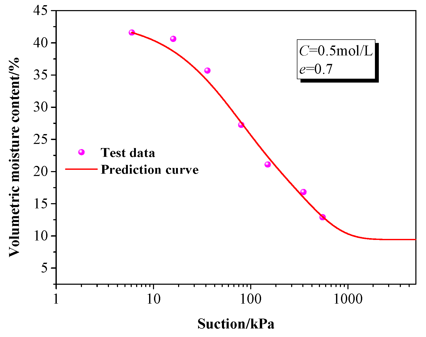
A new set of SWCC experimental data on the influence of salinity and deformation factors is selected [20], which is independent of the previous dataset. Using the trained model to predict volumetric water content under different suction conditions, the values of eight input variables such as salinity and void ratio are shown in Table 1. The range of matrix suction is 0–5000 kPa, with an interval of 100 kPa, and the output is the volume moisture content under corresponding conditions. The results obtained after calculation by the trained model are shown in Figure 5. It can be seen that for the SWCC considering the influence of deformation and salinity factors, the neural network prediction model has high prediction accuracy, especially in the low and medium suction stages.
In addition, a model prediction analysis was conducted on the variation in the characteristics of the SWCC under different void ratios and salinity conditions, and the input information is listed in Table 2. Figure 6 shows the simulated prediction results of the SWCC as a function of salinity under different void ratios. When the void ratio is constant, the SWCC has a tendency to move upwards with salinity, and this trend gradually increases as the void ratio increases.
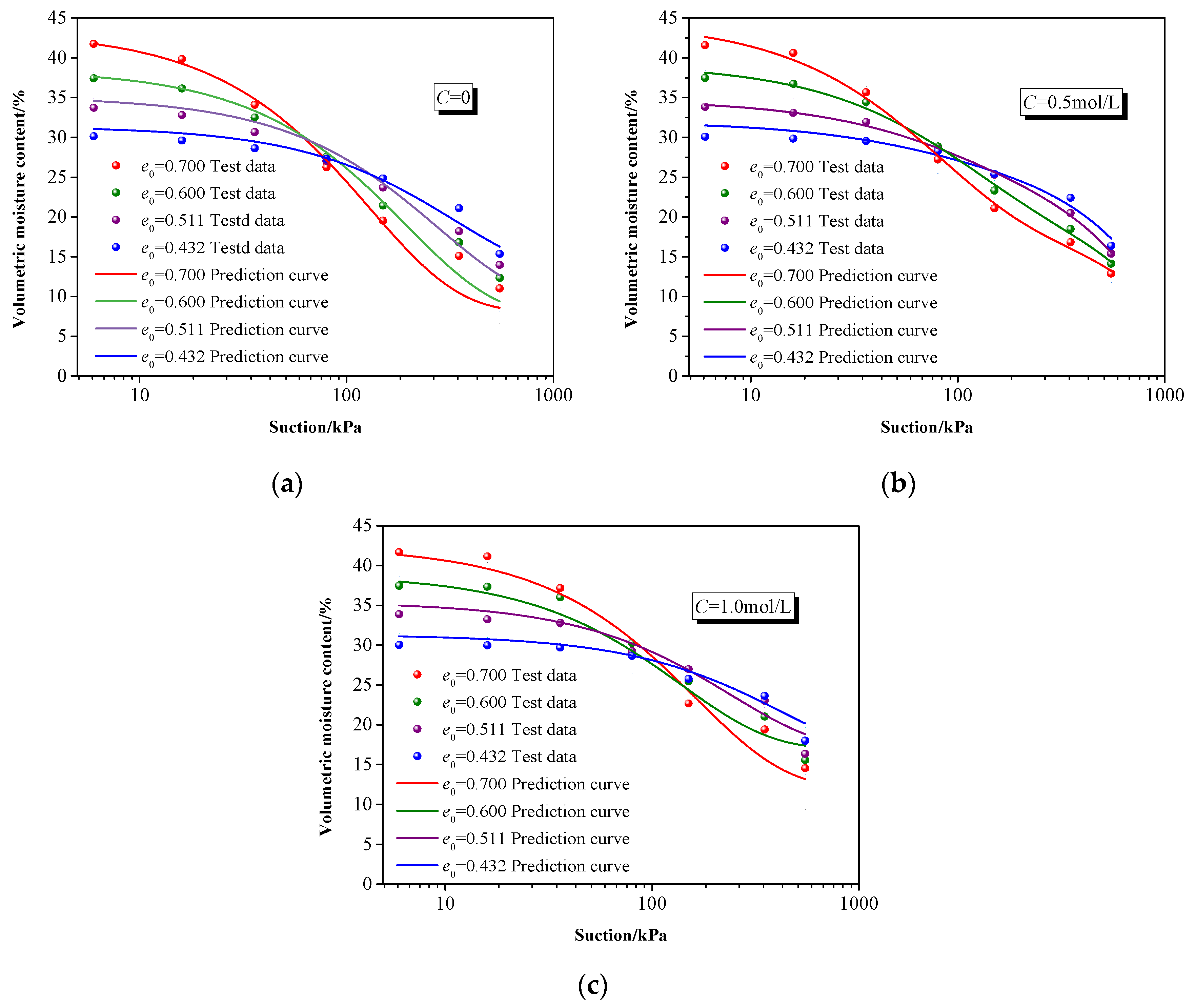
Under different salinities, the SWCC simulation with changes in the void ratio is shown in Figure 7. As the void ratio increases, the SWCC slope also increases. Meanwhile, as the salinity increases, the trend of an increasing SWCC slope slightly decreases. Overall, the model has a good prediction effect on the SWCC under different salinity and void ratio conditions.

3.2. SWCC Prediction Considering Temperature and Deformation Effects

Similarly, a set of new test data considering the effects of temperature and deformation is used to verify the predictive simulation ability of the model [18]. The input values of the model are shown in Table 3. The matrix suction range is 0–5000 kPa, and the interval is 100 kPa. The output is volume moisture content, and the prediction results are shown in Figure 8, which also shows a good prediction effect.
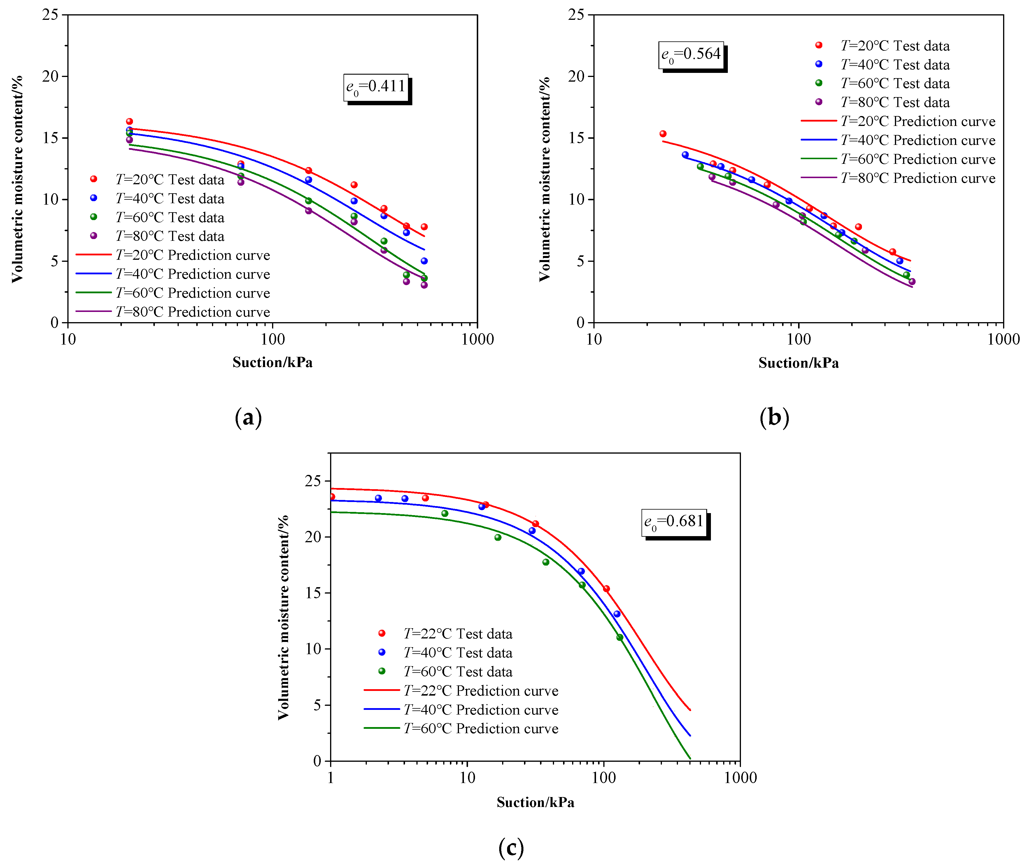
The SWCC under different temperatures and void ratios is predicted and analyzed. The input information is listed in Table 4 [46,47], and the predicted results are shown in Figure 9. At a certain void ratio, as the temperature increases, the SWCC shows a general downward trend. At the same time, as the void ratio increases, the degree of this downward movement decreases, and the slope of the SWCC also decreases accordingly. It can be seen that the model can well reflect this change characteristic.

3.3. SWCC Prediction Considering Temperature, Deformation, and Salinity Effects

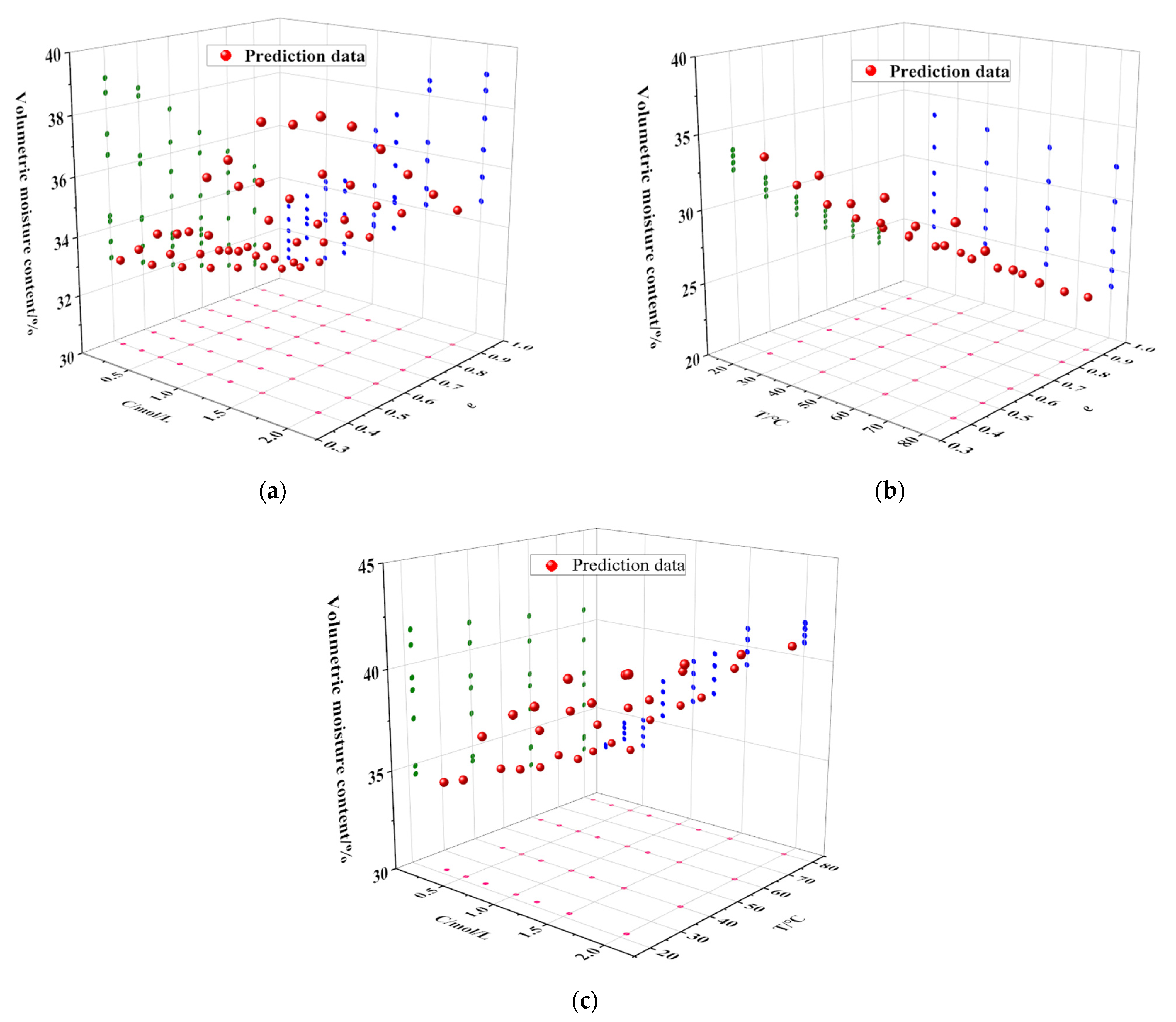
In order to more intuitively display the effects of temperature, deformation, and salinity on SWCC, some variables were randomly input, as shown in Table 5, for a three-dimensional display of the predicted results. Figure 10 shows the predicted results of the three-dimensional variation of volumetric water content with void ratio, temperature, and salinity under a certain matrix suction, as well as projections on different planes. The variation law of the volume water content under the influence of two factors, as well as the variation characteristics with one of the factors, can be obtained. For example, in Figure 10a, the variation in volumetric moisture content with salinity at a certain initial void ratio is shown in the w-C plane.
Figure 10 shows the predictive ability of the model on water retention characteristics under any two changing factors of salinity, void ratio, and temperature. Under the same suction condition (150 kPa), the prediction results of water retention capacity under different environmental factors are as follows: Figure 10a shows that the water retention capacity increases with increasing salinity and decreases with an increasing void ratio. The water retention capacity is more affected by salinity in the case of a smaller void ratio. Similarly, at a higher salinity, the water retention capacity is more affected by the void ratio. Figure 10b shows that the water retention capacity weakens with the increase in temperature and void ratio, and the influence of the void ratio is significantly stronger than that of temperature. There was little difference in the water retention capacity with temperature under different void ratios, and similarly, there was little difference in the water retention capacity with void ratios at different temperatures. Figure 10c shows that the magnitude of change in the water retention capacity decreases with an increasing temperature at a lower or higher salinity, and the effect of increasing soil–water retention capacity with increasing salinity was more pronounced with an increasing temperature.
Due to the scarcity of SWCC test data on the combined effects of temperature, deformation, and salinity, a model prediction analysis can only be conducted based on the existing data. A set of SWCC test data including the effects of void ratio and salinity was selected, with the temperature set to room temperature (22 °C), and the remaining input parameters set as shown in Table 6 [20]. The trained neural network model was used for prediction, and the predicted results were in good agreement with the experimental results, as shown in Figure 11. In addition, based on the above input values, the values of void ratio, salinity, and temperature were randomly changed, as shown in Table 6, and used as input variables for the model to predict the SWCC. From the prediction results in Figure 8, it can be seen that the random changes in temperature, void ratio, and salinity lead to different forms of changes in the SWCC, including overall movement, slope changes, changes in air entry value and residual moisture content. These indicate that the prediction model can adjust the SWCC according to the changes in input parameters.

4. Conclusions and Discussion

This paper focuses on the study of SWCC prediction under the influence of multiple factors by using a neural network machine learning approach, and the main conclusions are as follows:
(1)
Using neural network machine learning methods to train a large number of SWCC test results under complex environments, a SWCC prediction model that can consider the effects of multiple factors such as temperature, salinity, and deformation was obtained. The model selects the representative particle sizes d10/d30/d60, plasticity index, initial moisture content, void ratio, temperature, salinity, and matrix suction of the soil as input variables, and the volumetric moisture content as the output variable.
(2)
To improve the prediction accuracy of the model, separate training models were established for the SWCC considering temperature and deformation effects, as well as the SWCC considering salinity and deformation effects, for prediction analysis. By comparing the prediction results of the established model for SWCC characteristics under temperature, salinity, and deformation factors with relevant experimental results, including the effects of two factors and the combined effects of three factors, the validity of the model was verified.
(3)
The model directly takes environmental variables and the physical properties of the soil as inputs, overcoming the problem of poor prediction accuracy caused by the excessive number of parameters in traditional empirical formulas due to the increase in variables. In addition, this method takes suction conditions as input eigenvalues, which can directly obtain the corresponding water content under certain conditions, making it simpler and more direct.
The research results provide a new method for predicting SWCC under complex environmental influences, and can be combined with experimental data, empirical formulas, and other prediction methods to enhance the accuracy of SWCC prediction. However, there are still certain limitations to the research. The method of using neural networks for SWCC prediction must be based on a large amount of existing data. Due to the limited experimental data for the SWCC under the influence of multiple factors, the prediction accuracy of the prediction model obtained in this paper, by training with not too much experimental data, needs to be further improved.

Author Contributions

Conceptualization, G.Y. and Y.L.; methodology, N.W.; software, J.L.; validation, G.Y. and J.L.; formal analysis, G.Y.; investigation, J.L. and T.L.; resources, Y.L.; data curation, J.L. and T.L.; writing—original draft preparation, G.Y.; writing—review and editing, G.Y.; visualization, J.L.; supervision, N.W.; project administration, Y.L.; funding acquisition, G.Y. All authors have read and agreed to the published version of the manuscript.

Funding

The authors gratefully acknowledge the financial support provided by National Natural Science Foundation of China (No. 52108296) and the Interdisciplinary Research Project for Young Teachers of USTB (Fundamental Research Funds for the Central Universities) (No. FRF-IDRY-22-015).

Data Availability Statement

The original contributions presented in the study are included in the article, further inquiries can be directed to the corresponding author.

Conflicts of Interest

The authors declare no conflict of interest.

References

  1. Fredlund, D.G.; Rahardjo, H. Unsaturated Soil Mechanics in Engineering Practice; John Wiley & Sons, Inc.: Hoboken, NJ, USA, 2012. [Google Scholar]
  2. Zhai, Q.; Rahardjo, H.; Satyanaga, A.; Zhu, Y.; Dai, G.; Zhao, X. Estimation of wetting hydraulic conductivity function for unsaturated sandy soil. Eng. Geol. 2021, 285, 106034. [Google Scholar] [CrossRef]
  3. Satyanaga, A.; Rahardjo, H. Unsaturated shear strength of soil with bimodal soil water characteristic curve. Géotechnique 2019, 69, 828–832. [Google Scholar] [CrossRef]
  4. Al-Mahbashi, A.M.; Elkady, T.; Al-Shamrani, M. The Role of Stress States on the Hysteric Behavior of Expansive Soil under Multiple Drying-Wetting Cycles. Buildings 2023, 13, 1619. [Google Scholar] [CrossRef]
  5. Fredlund, D.G.; Xing, A. Equations for the soil-water characteristic curve. Can. Geotech. J. 1994, 31, 521–532. [Google Scholar] [CrossRef]
  6. Van Genuchten, M.T. A closed-form equation for predicting the hydraulic conductivity of unsaturated soils. Soil Sci. Soc. Am. J. 1980, 44, 892–898. [Google Scholar] [CrossRef]
  7. De la Morena, G.; Navarro, V.; Asensio, L.; Gallipoli, D. A water retention model accounting for void ratio changes in double porosity clays. Acta Geotech. 2021, 16, 2775–2790. [Google Scholar] [CrossRef]
  8. Lu, P.H.; He, Y.; Zhang, Z.; Ye, W.M. Predicting chemical influence on soil water retention curves with models established based on pore structure evolution of compacted clay. Comput. Geotech. 2021, 138, 104360. [Google Scholar] [CrossRef]
  9. Zhang, W.J.; Lin, M.F. Evaluating the dual porosity of landfilled municipal solid waste. Environ. Sci. Pollut. Res. 2019, 26, 12080–12088. [Google Scholar] [CrossRef]
  10. He, Y.F.; Lu, H.J.; Lan, J.R.; Ma, J.Y.; Liu, M.Y.; Dong, Y.Q. Macroscopic Mechanical Properties and Microstructure Characteristics of Solid Waste Base Capillary Retarded Field Covering Material. Buildings 2024, 14, 313. [Google Scholar] [CrossRef]
  11. Ma, C.Y.; Tang, L.B.; Chang, W.Q.; Jaffar, M.T.; Zhang, J.G.; Li, X.; Chang, Q.; Fan, J.L. Effect of Shelterbelt Construction on Soil Water Characteristic Curves in an Extreme Arid Shifting Desert. Water 2022, 14, 1803. [Google Scholar] [CrossRef]
  12. Zhu, J.H.; Su, Z.Y.; Zhang, H.Y. Soil-water characteristic curves and hydraulic conductivity of Gaomiaozi bentonite pellet-contained materials. Environ. Earth Sci. 2022, 81, 92. [Google Scholar] [CrossRef]
  13. Andry, H.; Yamamoto, T.; Irie, T.; Moritani, S.; Inoue, M.; Fujiyama, H. Water retention, hydraulic conductivity of hydrophilic polymers in sandy soil as affected by temperature and water quality. J. Hydrol. 2009, 373, 177–183. [Google Scholar] [CrossRef]
  14. He, Y.; Chen, Y.G.; Ye, W.M.; Chen, B.; Cui, Y.J. Influence of salt concentration on volume shrinkage and water retention characteristics of compacted GMZ bentonite. Environ. Earth Sci. 2016, 75, 535. [Google Scholar] [CrossRef]
  15. Pham, K.; Kim, D.; Le, C.V.; Won, J. Machine learning-based pedotransfer functions to predict soil water characteristics curves. Transp. Geotech. 2023, 42, 101052. [Google Scholar] [CrossRef]
  16. Gupta, S.; Papritz, A.; Lehmann, P.; Hengl, T.; Bonetti, S.; Or, D. Global Mapping of Soil Water Characteristics Parameters-Fusing Curated Data with Machine Learning and Environmental Covariates. Remote Sens. 2022, 14, 1947. [Google Scholar] [CrossRef]
  17. Li, Y.; Vanapalli, S.K. Prediction of soil-water characteristic curves using two artificial. Can. Geotech. J. 2022, 59, 129–143. [Google Scholar] [CrossRef]
  18. Uchaipichat, A.; Khalili, N. Experimental investigation of thermo-hydro-mechanical behavior of an unsaturated silt. Géotechnique 2009, 59, 339–353. [Google Scholar] [CrossRef]
  19. Li, X.Z. Experimental Study on Water Retention and Mechanical Behaviors of Saline Soil; Beijing Jiaotong University: Beijing, China, 2021. (In Chinese) [Google Scholar]
  20. Liu, Q.Q.; Li, J.; Cai, G.Q.; Li, P.L.; Li, X.Z. Experimental study on water retention characteristics of saline soil in the full suction range. Rock Soil Mech. 2021, 42, 713–722. (In Chinese) [Google Scholar]
  21. Zhai, Q.; Rahardjo, H. Determination of soil–water characteristic curve variables. Comput. Geotech. 2012, 42, 37–43. [Google Scholar] [CrossRef]
  22. Chen, P.; Liu, J.; Wei, C.F.; Xue, W.J.; Tian, H.H. Approach to Rapidly Determining the Water Retention Curves for Fine-Grained Soils in Capillary Regime Based on the NMR Technique. J. Eng. Mech. 2017, 143, 04017032. [Google Scholar] [CrossRef]
  23. Gallage, K.P.C.; Uchimura, T. Effects of Dry Density and Grain Size Distribution on Soil-Water Characteristic Curves of Sandy Soils. Soils Found. 2010, 50, 161–172. [Google Scholar] [CrossRef]
  24. Wang, M.; Pande, N.G.; Kong, W.L.; Feng, Y.T. Comparison of Pore-Size Distribution of Soils Obtained by Different Methods. Int. J. Geomech. 2016, 17, 06016012. [Google Scholar] [CrossRef]
  25. Antinoro, C.; Arnone, E.; Noto, L.V. The use of soil water retention curve models in analyzing slope stability in differently structured soils. CATENA 2017, 150, 133–145. [Google Scholar] [CrossRef]
  26. Pham, K.; Kim, D.; Yoon, Y.; Choi, H. Analysis of neural network based pedotransfer function for predicting soil water characteristic curve. Geoderma 2019, 351, 92–102. [Google Scholar] [CrossRef]
  27. Li, Y.Y.; Rahardjo, H.; Satyanaga, A.; Rangarajan, S.; Lee, D.T.T. Soil database development with the application of machine learning methods in soil properties prediction. Eng. Geol. 2022, 306, 106769. [Google Scholar] [CrossRef]
  28. Lu, P.H.; Ye, W.M.; He, Y. A constitutive model of compacted bentonite under coupled chemo-hydro-mechanical conditions based on the framework of the BExM. Comput. Geotech. 2023, 158, 105360. [Google Scholar] [CrossRef]
  29. Thyagaraj, T.; Rao, M.S. Influence of Osmotic Suction on the Soil-Water Characteristic Curves of Compacted Expansive Clay. J. Geotech. Geoenviron. Eng. 2010, 136, 1695–1702. [Google Scholar] [CrossRef]
  30. Yang, S.; Zheng, P.; Yu, Y.; Zhang, J. Probabilistic analysis of soil-water characteristic curve based on machine learning algorithms. IOP Conf. Ser. Earth Environ. Sci. 2021, 861, 062030. [Google Scholar] [CrossRef]
  31. Chen, Y.; Zhou, H.T.; Su, J.; Ye, R.Q.; Wang, L. Impact Analysis and Prediction Research of Soil-water Characteristic Curves Based on Data Mining. J. Basic Sci. Eng. 2023, 31, 451–466. (In Chinese) [Google Scholar]
  32. Prakash, A.; Hazra, B.; Sreedeep, S. Probabilistic analysis of soil-water characteristic curve using limited data. Appl. Math. Model. 2021, 89, 752–770. [Google Scholar] [CrossRef]
  33. Li, Y.; Vanapalli, S.K. A novel modeling method for the bimodal soil-water characteristic curve. Comput. Geotech. 2021, 138, 104318. [Google Scholar] [CrossRef]
  34. Ren, Q.B.; Li, M.C.; Han, S. Discrimination and comparison experiments of basalt tectonic setting based on improved genetic algorithm-optimized neural network. Earth Sci. Front. 2019, 26, 117–124. (In Chinese) [Google Scholar]
  35. Wang, L.; Li, D.Q.; Cao, Z.J.; Fang, G.G. Bayesian approaches for model selection and parameter identification of soil water characteristic curve. J. Basic Sci. Eng. 2019, 27, 1269–1284. (In Chinese) [Google Scholar]
  36. Chen, R.P.; Liu, P.; Liu, X.M.; Wang, P.F.; Kang, X. Pore-scale model for estimating the bimodal soil-water characteristic curve and hydraulic conductivity of compacted soils with different initial densities. Eng. Geol. 2019, 260, 105199. [Google Scholar] [CrossRef]
  37. Wang, T.H.; Lu, J.; Yue, C.K. Soil-water characteristic curve for unsaturated loess considering temperature and density effect. Rock Soil Mech. 2008, 29, 1–5. (In Chinese) [Google Scholar]
  38. Cai, G.Q.; Liu, Y.i.; Xu, R.Z.; Li, J.; Zhao, C.G. Experimental investigation for soil-water characteristic curve of red clay in full suction range. Chin. J. Geotech. Eng. 2019, 41, 13–16. (In Chinese) [Google Scholar]
  39. Sayem, H.M.; Kong, L.W. Effects of Drying-Wetting Cycles on Soil-Water Characteristic Curve. In Proceedings of the International Conference on Power Engineering and Energy, Environment (PEEE), Shanghai, China, 25–26 June 2016; pp. 607–614. [Google Scholar]
  40. Jiang, Y.; Chen, W.W.; Wang, G.H.; Sun, G.P.; Zhang, F.Y. Influence of initial dry density and water content on the soil–water characteristic curve and suction stress of a reconstituted loess soil. Bull. Eng. Geol. Environ. 2017, 76, 1085–1095. [Google Scholar] [CrossRef]
  41. Liu, W.P.; Luo, X.Y.; Fu, M.F.; Huang, J.S. Experiment and Modeling of Soil-Water Characteristic Curve of Unsaturated Soil in Collapsing Erosion Area. Pol. J. Environ. Stud. 2016, 25, 2509–2517. [Google Scholar] [CrossRef]
  42. Chen, R.; Tan, R.Q.; Chen, Z.K.; Ping, Y.; Mei, Z. Influence of degree of compaction on unsaturated hydraulic properties of a compacted completely decomposed granite. Geofluids 2020, 2020, 7615361. [Google Scholar] [CrossRef]
  43. Zhang, J.R.; Jiang, T.; Wang, X.C.; Liu, C.; Huang, Z.Q. Influences of drying and wetting cycles and compaction degree on strength of Yudong silt for subgrade and its prediction. Adv. Civ. Eng. 2018, 2018, 1364186. [Google Scholar] [CrossRef]
  44. Dai, Z.J.; Chen, S.X.; Luo, H.M.; Lu, D.J. Experimental study of water-holding and permeability characteristics of unsaturated expansive soils and rocks. Rock Soil Mech. 2013, 34, 134–141. (In Chinese) [Google Scholar]
  45. Cui, K.; Lin, W.K. Research on soil-water characteristic curve of unsaturated mixed-soil in Western Sichuan. China J. Highw. Transp. 2017, 30, 44–50. (In Chinese) [Google Scholar]
  46. Yao, Z.H.; Sun, F.X.; Fang, X.W.; Chen, Z.H. Water retention characteristics of unsaturated bentonite-sand mixtures under controlled-temperature. Environ. Earth Sci. 2021, 80, 315. [Google Scholar] [CrossRef]
  47. Gens, A. Specification of laboratory benchmark 3. Internal Document of Work Package 4. THERESA Proj. 2007, 91, 509–530. [Google Scholar]
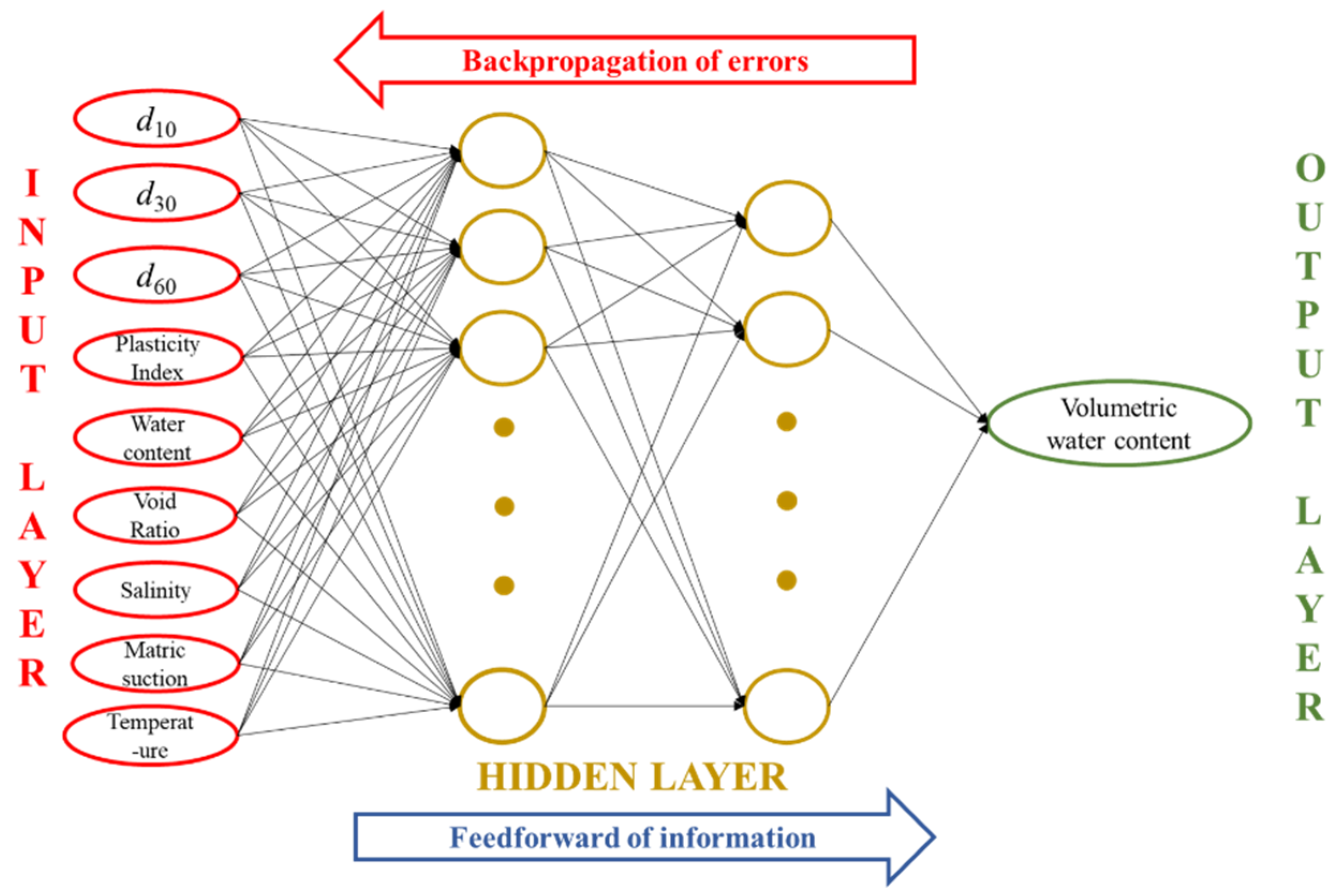
Figure 1. Construction of SWCC prediction model.
Buildings 14 02087 g001
Figure 2. Model training results of dataset 1: (a) Training: R = 0.97084; (b) Test: R = 0.95002; (c) All: R = 0.96711.
Buildings 14 02087 g002
Figure 3. Model training results of dataset 2: (a) Training: R = 0.96299; (b) Test: R = 0.87723; (c) All: R = 0.93431.
Buildings 14 02087 g003
Figure 4. Model training results of dataset 3: (a) Training: R = 0.90853; (b) Test: R = 0.94101; (c) All: R = 0.91251.
Buildings 14 02087 g004
Figure 5. SWCC prediction results considering the effects of salinity and void ratio.
Buildings 14 02087 g005
Figure 6. SWCC prediction with the change in salinity under different void ratio: (a) e0 = 0.7; (b) e0 = 0.6; (c) e0 = 0.511; (d) e0 = 0.432.
Buildings 14 02087 g006
Figure 7. SWCC prediction with the change in void ratio under different salinity: (a) C = 0; (b) C = 0.5 mol/L; (c) C = 1.0 mol/L.
Buildings 14 02087 g007
Figure 8. SWCC prediction results considering the effects of temperature and void ratio.
Buildings 14 02087 g008
Figure 9. SWCC prediction with the change in temperature under different void ratios: (a) e0 = 0.411; (b) e0 = 0.564; (c) e0 = 0.681.
Buildings 14 02087 g009
Figure 10. Three-dimensional scatter plot of SWCC prediction under the influence of two factors: (a) void ratio and salinity; (b) void ratio and temperature; (c) salinity and temperature.
Buildings 14 02087 g010
Figure 11. SWCC prediction considering the combined influence factors of temperature, salinity, and deformation.
Buildings 14 02087 g011
Table 1. The value of the input variables.
d10/mmd30/mmd60/mmIpw0e0C/mol·L−1s/kPa
0.00260.0210.06113.60.270.70.50–5000
Table 2. The value of the input variables.
d10/mmd30/mmd60/mmIpw0e0C/mol·L−1s/kPa
0.0030.0180.05312.2543.60.70/0.5/1.00–550
0.0030.0180.05312.2537.430.60/0.5/1.00–550
0.0030.0180.05312.2533.370.5110/0.5/1.00–550
0.0030.0180.05312.2530.140.4320/0.5/1.00–550
Table 3. The value of the input variables.
d10/mmd30/mmd60/mmIpw0e0T/°Cs/kPa
0.00210.0160.05815.80.360.76600–5000
Table 4. The value of the input variables.
d10/mmd30/mmd60/mmIpw0e0T/°Cs/kPa
0.00210.00260.06113.617/16/14/130.41120/40/60/800–500
0.00210.00260.06113.614/13/12.5/11.50.56420/40/60/800–500
0.0160.0360.0649.4224/23/220.68122/40/600–500
Table 5. The value of the input variables.
d10/mmd30/mmd60/mmIpw0e0T/°CC/mol·L−1s/kPa
0.0250.0870.2212.5350.4–0.920–800150
0.0250.0870.2212.5250.4–0.9220.1–2.0150
0.0250.0870.2212.5300.720–800.1–2.0150
Table 6. The value of the input nodes.
d10/mmd30/mmd60/mmIpw0e0T/°CC/mol·L−1s/kPa
0.0030.0180.05312.25410.72210–1000
0.0030.0180.05312.25410.6500.50–1000
0.0030.0180.05312.25410.4801.50–1000
0.0030.0180.05312.25410.8600.10–1000
Disclaimer/Publisher’s Note: The statements, opinions and data contained in all publications are solely those of the individual author(s) and contributor(s) and not of MDPI and/or the editor(s). MDPI and/or the editor(s) disclaim responsibility for any injury to people or property resulting from any ideas, methods, instructions or products referred to in the content.