
Exploring Performance of Using SCM Concrete: Investigating Impacts Shifting along Concrete Supply Chain and Construction
Abstract
:1. Introduction
2. Background
3. Method
3.1. Collection
3.2. Simulation
3.3. Calculation
3.4. Decision
4. Case Study
4.1. Case Background
4.2. Temperature during Construction
4.3. Concrete Data
5. Results
5.1. GHG Emissions
5.2. Cost
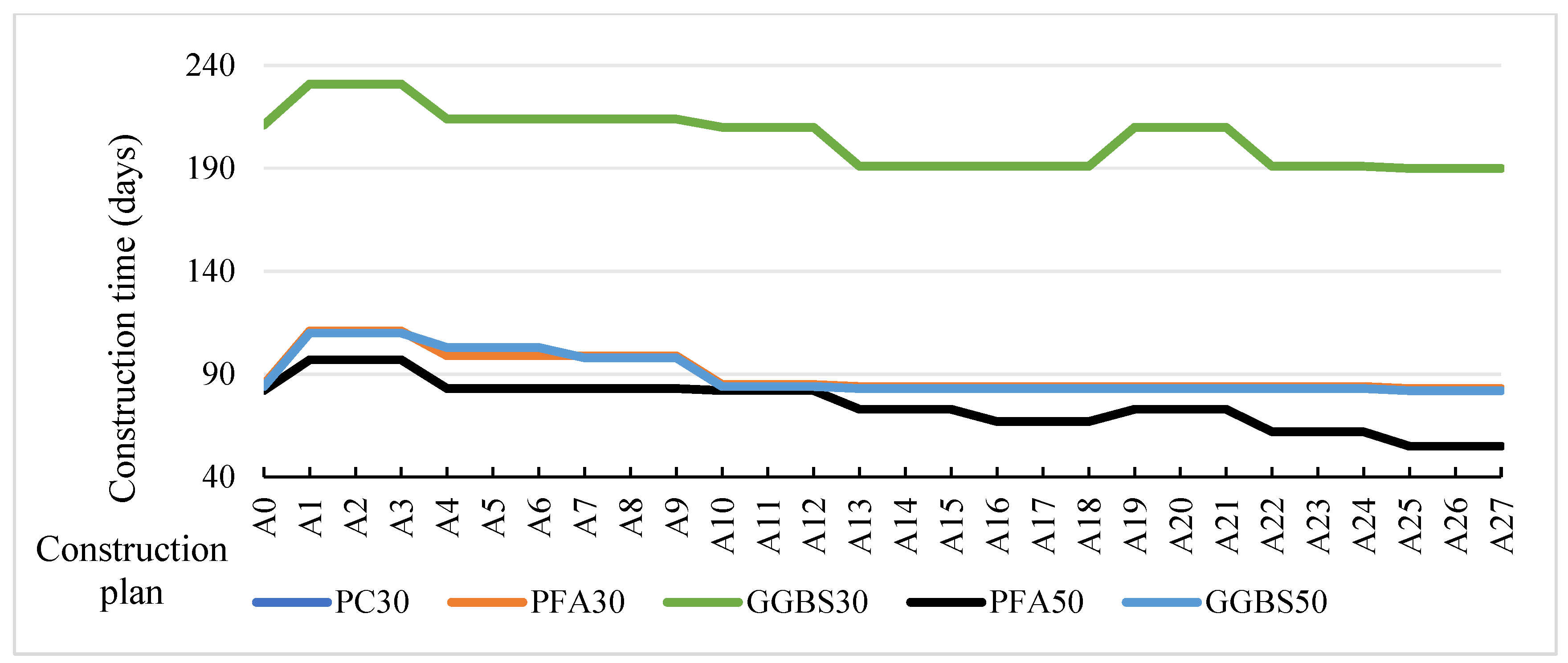
5.3. Time
5.4. Selection of Concrete Type
6. Discussion
6.1. Method and Result Comparison
6.2. Scenario Analysis
6.2.1. Scenarios with Changed GWP Factors
6.2.2. Scenarios with Changed Surrounding Temperature
6.2.3. Scenarios with Changed Construction Plans
7. Conclusions
Author Contributions
Funding
Data Availability Statement
Conflicts of Interest
Abbreviations
| CSCD method | Collection–Simulation–Calculation–Decision method |
| DES | Discrete event simulation |
| FA | Fly ash |
| GGBS | Ground granulated blast furnace slag |
| GGBS30 | Concrete using ground granulated blast furnace slag with compressive strength of 30 MPa |
| GGBS50 | Concrete using ground granulated blast furnace slag with compressive strength of 50 MPa |
| GHG | Greenhouse gas |
| GWP | Global warming potential |
| LCA | Life cycle assessment |
| PC30 | Ordinary Portland cement concrete with compressive strength of 30 MPa |
| PFA30 | Concrete using fly ash with compressive strength of 30 MPa |
| PFA50 | Concrete using fly ash with compressive strength of 50 MPa |
| SCM | Supplementary cementitious materials |
References
- Miller, S.; Horvath, A.; Monteiro, P. Readily implementable techniques can cut annual CO2 emissions from the production of concrete by over 20%. Environ. Res. Lett. 2016, 11, 074029. [Google Scholar] [CrossRef]
- Scrivener, K.L.; John, V.M.; Gartner, E.M. Eco-efficient cements: Potential economically viable solutions for a low-CO2 cement-based materials industry. Cem. Concr. Res. 2018, 114, 2–26. [Google Scholar] [CrossRef]
- Benhelal, E.; Zahedi, G.; Shamsaei, E.; Bahadori, A. Global strategies and potentials to curb CO2 emissions in cement industry. J. Clean. Prod. 2013, 51, 142–161. [Google Scholar] [CrossRef]
- Mala, K.; Mullick, A.K.; Jain, K.K.; Singh, P.K. Effect of Relative Levels of Mineral Admixtures on Strength of Concrete with Ternary Cement Blend. Int. J. Concr. Struct. Mater. 2013, 7, 239–249. [Google Scholar] [CrossRef]
- Costa, F.N.; Ribeiro, D.V. Reduction in CO2 emissions during production of cement, with partial replacement of traditional raw materials by civil construction waste (CCW). J. Clean. Prod. 2020, 276, 123302. [Google Scholar] [CrossRef]
- Nwankwo, C.O.; Bamigboye, G.O.; Davies, I.E.E.; Michaels, T.A. High volume Portland cement replacement: A review. Constr. Build. Mater. 2020, 260, 120445. [Google Scholar] [CrossRef]
- Bianco, I.; Ap Dafydd Tomos, B.; Vinai, R. Analysis of the environmental impacts of alkali-activated concrete produced with waste glass-derived silicate activator—A LCA study. J. Clean. Prod. 2021, 316, 128383. [Google Scholar] [CrossRef]
- Yang, K.-H.; Jung, Y.-B.; Cho, M.-S.; Tae, S.-H. Effect of supplementary cementitious materials on reduction of CO2 emissions from concrete. Carbon Emiss. Reduct. Policies Technol. Monit. Assess. Model. 2015, 103, 774–783. [Google Scholar] [CrossRef]
- Göswein, V.; Gonçalves, A.B.; Silvestre, J.D.; Freire, F.; Habert, G.; Kurda, R. Transportation matters—Does it? GIS-based comparative environmental assessment of concrete mixes with cement, fly ash, natural and recycled aggregates. Resour. Conserv. Recycl. 2018, 137, 1–10. [Google Scholar] [CrossRef]
- Samad, S.; Shah, A. Role of binary cement including Supplementary Cementitious Material (SCM), in production of environmentally sustainable concrete: A critical review. Int. J. Sustain. Built Environ. 2017, 6, 663–674. [Google Scholar] [CrossRef]
- Dhir, R.K.; McCarthy, M.J.; Paine, K.A. Engineering property and structural design relationships for new and developing concretes. Mater. Struct. 2005, 38, 1–9. [Google Scholar] [CrossRef]
- Khatib, J.M.; Hibbert, J.J. Selected engineering properties of concrete incorporating slag and metakaolin. Constr. Build. Mater. 2005, 19, 460–472. [Google Scholar] [CrossRef]
- Dharek, M.S.; M, M.; S, B.; Vengala, J.; Tangadagi, R.B. Performance evaluation of hybrid fiber reinforced concrete on engineering properties and life cycle assessment: A sustainable approach. J. Clean. Prod. 2024, 458, 142498. [Google Scholar] [CrossRef]
- International Energy Agency (IEA); World Business Council for Sustainable Development (WBCSD). Cement Technology Roadmap 2009: Carbon Emissions Reductions up to 2050; International Energy Agency (IEA): Paris, France, 2009.
- Miller, S.A.; John, V.M.; Pacca, S.A.; Horvath, A. Carbon dioxide reduction potential in the global cement industry by 2050. Cem. Concr. Res. 2018, 114, 115–124. [Google Scholar] [CrossRef]
- Our World in Data. Annual CO2 emissions from Cement, 2022 [WWW Document]. 2024. Available online: https://ourworldindata.org/grapher/annual-co2-cement?country=CHN~USA~IND~ZAF~AUS~OWID_EUR~TUR~SAU~IDN~BRA~KOR~JPN~RUS~IRN~MEX~THA~VNM~OWID_AFR#explore-the-data (accessed on 9 February 2024).
- Miller, S.A. Supplementary cementitious materials to mitigate greenhouse gas emissions from concrete: Can there be too much of a good thing? J. Clean. Prod. 2018, 178, 587–598. [Google Scholar] [CrossRef]
- Potting, J.; Hekkert, M.P.; Worrell, E.; Hanemaaijer, A. Circular Economy: Measuring Innovation in the Product Chain; PBL Netherlands Assessment Agency: The Hague, The Netherlands, 2017. [Google Scholar]
- Mohammed Owaid, H.; Hamid, R.B.; Taha, M.R. A Review of Sustainable Supplementary Cementitious Materials as an Alternative to All-Portland Cement Mortar and Concrete. Aust. J. Basic Appl. Sci. 2012, 6, 287–303. [Google Scholar]
- Yaseen, N.; Alcivar-Bastidas, S.; Irfan-ul-Hassan, M.; Petroche, D.M.; Qazi, A.U.; Ramirez, A.D. Concrete incorporating supplementary cementitious materials: Temporal evolution of compressive strength and environmental life cycle assessment. Heliyon 2024, 10, e25056. [Google Scholar] [CrossRef] [PubMed]
- Juenger, M.C.G.; Siddique, R. Recent advances in understanding the role of supplementary cementitious materials in concrete. Cem. Concr. Res. 2015, 78, 71–80. [Google Scholar] [CrossRef]
- Chen, C.; Habert, G.; Bouzidi, Y.; Jullien, A.; Ventura, A. LCA allocation procedure used as an incitative method for waste recycling: An application to mineral additions in concrete. Resour. Conserv. Recycl. 2010, 54, 1231–1240. [Google Scholar] [CrossRef]
- Soutsos, M.; Hatzitheodorou, A.; Kwasny, J.; Kanavaris, F. Effect of in situ temperature on the early age strength development of concretes with supplementary cementitious materials. Constr. Build. Mater. 2016, 103, 105–116. [Google Scholar] [CrossRef]
- Ballim, Y.; Graham, P.C. The effects of supplementary cementing materials in modifying the heat of hydration of concrete. Mater. Struct. 2009, 42, 803–811. [Google Scholar] [CrossRef]
- Lu, W.; Olofsson, T. Building information modeling and discrete event simulation: Towards an integrated framework. Autom. Constr. 2014, 44, 73–83. [Google Scholar] [CrossRef]
- AbouRizk, S.; Halpin, D.; Mohamed, Y.; Hermann, U. Research in Modeling and Simulation for Improving Construction Engineering Operations. J. Constr. Eng. Manag. 2011, 137, 843–852. [Google Scholar] [CrossRef]
- Creighton, D.; Nahavandi, S. Application of discrete event simulation for robust system design of a melt facility. Leadersh. Future Manuf. 2003, 19, 469–477. [Google Scholar] [CrossRef]
- AbouRizk, S. Role of Simulation in Construction Engineering and Management. J. Constr. Eng. Manag. 2010, 136, 1140–1153. [Google Scholar] [CrossRef]
- Zhang, H.; Li, H. Simulation-based optimization for dynamic resource allocation. Autom. Constr. 2004, 13, 409–420. [Google Scholar] [CrossRef]
- Li, H.X.; Zhang, L.; Mah, D.; Yu, H. An integrated simulation and optimization approach for reducing CO2 emissions from on-site construction process in cold regions. Energy Build. 2017, 138, 666–675. [Google Scholar] [CrossRef]
- Feng, K.; Lu, W.; Chen, S.; Wang, Y. An Integrated Environment–Cost–Time Optimisation Method for Construction Contractors Considering Global Warming. Sustainability 2018, 10, 4207. [Google Scholar] [CrossRef]
- Saul, A. Principles underlying the steam curing of concrete at atmospheric pressure. Mag. Concr. Res. 1951, 2, 127–140. [Google Scholar] [CrossRef]
- Poole, T.; Harrington, P. An Evaluation of the Maturity Method (ASTM C 1074) for Use in Mass Concrete; US Army Corps of Engineers: Washington, DC, USA, 1996. [Google Scholar]
- ASTM C1074-11; Standard Practice for Estimating Concrete Strength by the Maturity Method. American Society of Testing and Materials (ASTM): West Conshohocken, PA, USA, 2011.
- Carino, N. The Maturity Method: Theory and Application. Cem. Concr. Aggreg. 1984, 6, 61–73. [Google Scholar] [CrossRef]
- Vollpracht, A.; Soutsos, M.; Kanavaris, F. Strength development of GGBS and fly ash concretes and applicability of fib model code’s maturity function—A critical review. Constr. Build. Mater. 2018, 162, 830–846. [Google Scholar] [CrossRef]
- Fischer, M.; Aalami, F.; Kuhne, C.; Ripberger, A. Cost-loaded production model for planning and control. In Durability of Building Materials and Components 8; Proceedings; Lacasse, M.A., Vainer, D.J., Eds.; National Research Council Canada: Ottawa, ON, Canada, 1999; Volume 1–4, pp. 2813–2824. [Google Scholar]
- Dehghanimohammadabadi, M.; Keyser, T.K. Intelligent simulation: Integration of SIMIO and MATLAB to deploy decision support systems to simulation environment. Simul. Model. Pract. Theory 2017, 71, 45–60. [Google Scholar] [CrossRef]
- Refaa, Z.; Kakar, M.R.; Stamatiou, A.; Worlitschek, J.; Partl, M.N.; Bueno, M. Numerical study on the effect of phase change materials on heat transfer in asphalt concrete. Int. J. Therm. Sci. 2018, 133, 140–150. [Google Scholar] [CrossRef]
- Angervall, T.; Flysjö, A.; Mattsson, B. Jämförelse av Dricksvatten-Översiktlig Livscykelanalys (LCA); The Swedish Institute for Food and Biotechnology (SIK): Göteborg, Sweden, 2004. [Google Scholar]
- Ji, L.; Liang, S.; Qu, S.; Zhang, Y.; Xu, M.; Jia, X.; Jia, Y.; Niu, D.; Yuan, J.; Hou, Y.; et al. Greenhouse gas emission factors of purchased electricity from interconnected grids. Appl. Energy 2016, 184, 751–758. [Google Scholar] [CrossRef]
- National Meteorological Centre (NMC) of China. Weather Statistics for Beijing [WWW Document]. 2019. Available online: http://www.nmc.cn/publish/forecast/ABJ/beijing.html (accessed on 10 January 2024).
- Deb, K. Multiobjective Optimization Using Evolutionary Algorithms; John Wiley & Sons Inc.: Hoboken, NJ, USA, 2001. [Google Scholar]
- Feng, K.; Lu, W.; Olofsson, T.; Chen, S.; Yan, H.; Wang, Y. A Predictive Environmental Assessment Method for Construction Operations: Application to a Northeast China Case Study. Sustainability 2018, 10, 3868. [Google Scholar] [CrossRef]
- Olsson, J.A.; Miller, S.A.; Kneifel, J.D. A review of current practice for life cycle assessment of cement and concrete. Resour. Conserv. Recycl. 2024, 206, 107619. [Google Scholar] [CrossRef]
- Hong, J.; Shen, G.Q.; Mao, C.; Li, Z.; Li, K. Life-cycle energy analysis of prefabricated building components: An input–output-based hybrid model. J. Clean. Prod. 2016, 112, 2198–2207. [Google Scholar] [CrossRef]
- Sánchez, A.R.; Ramos, V.C.; Polo, M.S.; Ramón, M.V.L.; Utrilla, J.R. Life Cycle Assessment of Cement Production with Marble Waste Sludges. Int. J. Environ. Res. Public Health 2021, 18, 10968. [Google Scholar] [CrossRef] [PubMed]
- Georgiades, M.; Shah, I.H.; Steubing, B.; Cheeseman, C.; Myers, R.J. Prospective life cycle assessment of European cement production. Resour. Conserv. Recycl. 2023, 194, 106998. [Google Scholar] [CrossRef]
- Tokareva, A.; Kaassamani, S.; Waldmann, D. Fine demolition wastes as Supplementary cementitious materials for CO2 reduced cement production. Constr. Build. Mater. 2023, 392, 131991. [Google Scholar] [CrossRef]
- Itten, R.; Frischknecht, R.; Stucki, M. Life Cycle Inventories of Electricity Mixes and Grid; Paul Scherrer Institute (PSI): Villigen, Switzerland, 2014. [Google Scholar]
- Department of the Environment and Energy-Australian Government. National Greenhouse Gas Accounts Factors; Department of the Environment and Energy-Australian Government: Parkes, Australia, 2018.
- Kaatz, J.; Anders, S. The role of unspecified power in developing locally relevant greenhouse gas emission factors in California’s electric sector. Electr. J. 2016, 29, 1–11. [Google Scholar] [CrossRef]
- Canada Energy Regulator. Market Snapshot: Greenhouse Gas Emissions Associated with Residential Electricity Consumption Vary Significantly by Province and Territory [WWW Document]. 2017. Available online: https://www.cer-rec.gc.ca/nrg/ntgrtd/mrkt/snpsht/2017/06-04grngsmssnsrsdntl-eng.html (accessed on 10 January 2024).


| Phase | GWP Factor | Reference | |
|---|---|---|---|
| Raw materials exploitation (A1) | Cement | 0.931 kg CO2-eq/kg | [8] |
| Ground granulated blast furnace slag | 0.0265 kg CO2-eq/kg | ||
| Fly ash | 0.0196 kg CO2-eq/kg | ||
| Sand | 0.0026 kg CO2-eq/kg | ||
| Gravel | 0.0075 kg CO2-eq/kg | ||
| Water | 0.0000321 kg CO2-eq/kg | [40] | |
| Raw material transportation (A2) | Cement | 0.0000518 kg CO2-eq/(kg km) | [8] |
| Ground granulated blast furnace slag | 0.0000518 kg CO2-eq/(kg km) | ||
| Fly ash | 0.0000518 kg CO2-eq/(kg km) | ||
| Sand | 0.000063 kg CO2-eq/(kg km) | ||
| Gravel | 0.000063 kg CO2-eq/(kg km) | ||
| Concrete production (A3) | Fresh concrete production | 0.00768 kg CO2-eq/kg | [8] |
| Concrete transportation (A4) | Concrete transportation | 0.674 kg CO2-eq/(m3 km) | [8] |
| Construction (A5) | Electricity | 0.945 kg CO2-eq/kWh | [41] |
| Concrete Type | 28-Day Compressive Strength (MPa) | Cement (kg/m3) | Water (kg/m3) | Gravel (kg/m3) | Sand (kg/m3) | SCM (kg/m3) | Density (kg/m3) |
|---|---|---|---|---|---|---|---|
| PC30 | 30 | 240 | 158 | 1102 | 799 | 0 | 2299 |
| PFA30 | 30 | 193 | 144 | 1319 | 560 | 82 (30%) | 2298 |
| GGBS30 | 30 | 115 | 150 | 1187 | 721 | 115 (50%) | 2288 |
| PFA50 | 50 | 270 | 135 | 1250 | 533 | 115 (30%) | 2303 |
| GGBS50 | 50 | 165 | 165 | 1151 | 683 | 165 (50%) | 2329 |
| Process | Activity | Quantity (Q) | GWP Factors (GWP) | GHG Emissions (kg CO2-eq) Q × GWP |
|---|---|---|---|---|
| A1 | Production of cement | 240 kg | 0.931 kg CO2-eq/kg | 223.440 |
| Production of sand | 799 kg | 0.0026 kg CO2-eq/kg | 2.077 | |
| Production of gravel | 1102 kg | 0.0075 kg CO2-eq/kg | 8.265 | |
| Production of water | 158 kg | 0.0000321 kg CO2-eq/kg | 0.005 | |
| A2 | Transportation of cement | 194 km | 0.0000518 kg CO2-eq/(kg km) | 2.412 |
| Transportation of sand | 40 km | 0.000063 kg CO2-eq/(kg km) | 2.013 | |
| Transportation of gravel | 35 km | 0.000063 kg CO2-eq/(kg km) | 2.430 | |
| A3 | Production of fresh concrete | 2299 kg | 0.00768 kg CO2-eq/kg | 17.656 |
| A4 | Transportation of concrete | 43 km | 0.674 kg CO2-eq/(m3 km) | 28.982 |
| A1~A4 Total | 287.281 | |||
| Concrete Type | PC30 | PFA30 | GGBS30 | PFA50 | GGBS50 |
|---|---|---|---|---|---|
| Calculation results of this study | 287.281 | 246.468 | 174.510 | 319.181 | 223.298 |
| Concrete Type | PC30 | PFA30 | GGBS30 | PFA50 | GGBS50 |
|---|---|---|---|---|---|
| Buying price (Yuan/m3) | 550 | 435 | 320 | 640 | 450 |
| Concrete Type | a | b | c | d | R2 |
|---|---|---|---|---|---|
| PC30 | 57.57 | −0.00111 | −38.31 | −0.04302 | 0.9893 |
| PFA30 | 52.68 | 0.0001855 | −32.83 | −0.05393 | 0.9992 |
| GGBS30 | 60 | −0.001804 | −41 | −0.01902 | 0.9973 |
| PFA50 | 63.88 | −0.0004385 | −44.07 | −0.053 | 0.9993 |
| GGBS50 | 78.08 | −0.001857 | −58.36 | −0.02758 | 0.9990 |
| Concrete Type | a | b | c | d | R2 |
|---|---|---|---|---|---|
| PC30 | 73.55 | 370.1 | 2.18 | 230.5 | 0.9821 |
| PFA30 | 47.02 | −14.95 | 1.023 | 218.7 | 0.9978 |
| GGBS30 | 17.55 | −108.5 | 0.4758 | 179.2 | 0.9968 |
| PFA50 | 40.37 | 79.08 | 0.6412 | 81.28 | 0.9971 |
| GGBS50 | 47.71 | 189.6 | 0.8597 | 307 | 0.9971 |
| Concrete Type | Quantified Supply Chain GHG Emissions (kg CO2-eq/m2) | Quantified Supply Chain GHG Emissions (kg CO2-eq/m3) | Supply Chain GHG Emissions in Circular Ecology (kg CO2-eq/m3) | Difference Ratio (%) |
|---|---|---|---|---|
| PC30 | 102.9 | 270.1 | 257 | −4.8 |
| PFA30 | 88.3 | 231.8 | 214 | −7.7 |
| GGBS30 | 62.5 | 164.1 | 147 | −10.4 |
| PFA50 | 114.3 | 300.1 | 284 | −5.4 |
| GGBS50 | 80.0 | 210.0 | 195 | −7.1 |
| Concrete Type | GHG Emissions (kg CO2-eq/m2) | Cost (Yuan/m2) | Time (days) | Selection |
|---|---|---|---|---|
| PC30 | 299.0 | 120.3 | 85 | Basic scenario, Not Pareto solution |
| PFA30 | 260.7 (−12.8%) | 107.0 (−11.1%) | 85 (±0%) | Lowest GHG emissions, Pareto solution |
| GGBS30 | 339.3 (+13.5%) | 119.0 (−1.1%) | 211 (+148.2%) | Not Pareto solution |
| PFA50 | 297.0 (−0.7%) | 121.3 (+0.8%) | 82 (−3.5%) | Shortest duration, Pareto solution |
| GGBS50 | 264.7 (−11.4%) | 98.3 (−18.3%) | 84 (−1.2%) | Smallest cost, Pareto solution |
| Countries and Locations | GWP Factors (kg CO2-eq/kWh) | Reference | |
|---|---|---|---|
| Sweden | 0.056 | [50] | |
| China | South China | 0.398 | [41] |
| Central China | 0.573 | ||
| East China | 0.749 | ||
| North China (including Beijing) | 0.945 | ||
| Northwest China | 0.995 | ||
| Northeast China | 1.197 | ||
| Australia | Victoria | 1.070 | [51] |
| Queensland | 0.800 | ||
| South Australia | 0.510 | ||
| USA | California | 0.428 | [52] |
| Canada | Alberta | 0.950 | [53] |
| Northwest Territories | 0.500 | ||
| Prince Edward Island | 0.280 | ||
| No. | Carpenters | Concrete Workers | Wall Heaters’ Heat Transfer Coefficient (W/(m2 K)) | No. | Carpenters | Concrete Workers | Wall Heaters’ Heat Transfer Coefficient (W/(m2 K)) |
|---|---|---|---|---|---|---|---|
| A0 | 10 | 10 | 1.8 | A14 | 15 | 15 | 1.8 |
| A1 | 5 | 10 | 0.9 | A15 | 15 | 15 | 2.7 |
| A2 | 5 | 10 | 1.8 | A16 | 15 | 20 | 0.9 |
| A3 | 5 | 10 | 2.7 | A17 | 15 | 20 | 1.8 |
| A4 | 5 | 15 | 0.9 | A18 | 15 | 20 | 2.7 |
| A5 | 5 | 15 | 1.8 | A19 | 25 | 10 | 0.9 |
| A6 | 5 | 15 | 2.7 | A20 | 25 | 10 | 1.8 |
| A7 | 5 | 20 | 0.9 | A21 | 25 | 10 | 2.7 |
| A8 | 5 | 20 | 1.8 | A22 | 25 | 15 | 0.9 |
| A9 | 5 | 20 | 2.7 | A23 | 25 | 15 | 1.8 |
| A10 | 15 | 10 | 0.9 | A24 | 25 | 15 | 2.7 |
| A11 | 15 | 10 | 1.8 | A25 | 25 | 20 | 0.9 |
| A12 | 15 | 10 | 2.7 | A26 | 25 | 20 | 1.8 |
| A13 | 15 | 15 | 0.9 | A27 | 25 | 20 | 2.7 |
Disclaimer/Publisher’s Note: The statements, opinions and data contained in all publications are solely those of the individual author(s) and contributor(s) and not of MDPI and/or the editor(s). MDPI and/or the editor(s) disclaim responsibility for any injury to people or property resulting from any ideas, methods, instructions or products referred to in the content. |
© 2024 by the authors. Licensee MDPI, Basel, Switzerland. This article is an open access article distributed under the terms and conditions of the Creative Commons Attribution (CC BY) license (https://creativecommons.org/licenses/by/4.0/).
Share and Cite
Chen, S.; Ye, Z.; Lu, W.; Feng, K. Exploring Performance of Using SCM Concrete: Investigating Impacts Shifting along Concrete Supply Chain and Construction. Buildings 2024, 14, 2186. https://doi.org/10.3390/buildings14072186
Chen S, Ye Z, Lu W, Feng K. Exploring Performance of Using SCM Concrete: Investigating Impacts Shifting along Concrete Supply Chain and Construction. Buildings. 2024; 14(7):2186. https://doi.org/10.3390/buildings14072186
Chicago/Turabian StyleChen, Shiwei, Zhukai Ye, Weizhuo Lu, and Kailun Feng. 2024. "Exploring Performance of Using SCM Concrete: Investigating Impacts Shifting along Concrete Supply Chain and Construction" Buildings 14, no. 7: 2186. https://doi.org/10.3390/buildings14072186