Modeling and Assessment of Temperature and Thermal Stress Field of Asphalt Pavement on the Tibetan Plateau

Abstract

The Qinghai–Tibet Plateau (QTP) is the highest altitude plateau in the world, characterized by strong solar radiation and large diurnal temperature differences and so on, which brings a great negative impact on the temperature and thermal stress field of asphalt pavement. The purpose of this study is to analyze the temperature field and thermal stress status of asphalt pavement in the QTP to provide a reference for pavement design and maintenance in high-altitude areas. The finite element method was applied to establish the temperature field model to study the distribution and variation of pavement temperature. On this basis, the influence of cooling amplitude on pavement thermal stress was studied during cold waves. In addition to this, the key internal factors affecting the thermal stress of pavement, such as surface thickness, surface temperature shrinkage coefficient, surface modulus, and base modulus, were analyzed by an orthogonal test. It was found that temperature and solar radiation have a significant effect on the pavement temperature field. When the cold wave came, the cooling rate had a considerable impact on the thermal stress of the pavement, that is, every 5 °C increase in cooling rate would increase the thermal stress by more than 50%. The temperature shrinkage coefficient and surface modulus of the surface layer material had the greatest influence on the pavement thermal stress. The thermal stress could be reduced by more than 0.4 Mpa for every 5 × 10⁻⁶/°C reduction in the surface temperature shrinkage coefficient or every 1000 Mpa reduction in the surface modulus. This study can provide a reference for improving the temperature field and thermal stress field of asphalt pavement in the plateau area.

1. Introduction

The QTP, the youngest and highest plateau on Earth, is known as the “third pole” of the planet, which exerts influence on global climate change and is rich in mineral resources [1,2,3]. It appears to have long been a focus of attention for researchers in domestic and overseas. Apparently, the construction of the QTP road is of crucial interest to scientific research and resource development. Nevertheless, its average altitude of 4500 m indicates its harsh climatic conditions, such as low temperature, strong solar radiation, and large diurnal temperature difference. The mean temperature in the cold season is below -10 °C and the daily temperature variation is above 15 °C [4,5]. The performance of asphalt pavements is highly susceptible to environmental influences, notably the spheric temperature. More to the point, the thermal stress of asphalt pavement is dramatically increased under the combined effect of low temperature and cold waves [6,7,8]. Asphalt pavements are significantly affected by solar radiation and external atmospheric convective exchanges, which can lead to the formation of different temperature gradients within the pavement, causing different degrees of temperature strain and thus different degrees of thermal stress. And when the temperature is lower, the tensile strength of the asphalt mixture decreases. The coupling of temperature and vehicle loading makes the stress greater than the tensile strength of the asphalt mixture, which leads to thermal cracks in the asphalt pavement. Water entering the pavement structure along the cracks will cause erosion, spalling, loosening, and other diseases. This contributes to the frequent occurrence of cracks on the QTP [9,10,11] (Figure 1).

Numerous studies demonstrated that the characteristics of asphalt can be critically affected by temperature [12,13,14]. As a consequence, the process of heat transfer in asphalt pavements is of great significance and it affects the properties of asphalt pavements [15,16,17,18]. There were extensive studies on the temperature and thermal stress fields of asphalt pavements. First of all, Barber et al. [19] researched the association of pavement temperature with environmental conditions such as solar radiation, wind velocity, and atmospheric temperature, and introduced the first theoretical analysis approach for predicting pavement temperature. Based on the finite difference method, Christison et al. [20] developed software that can predict the temperature field of pavement using continuous temperature records from several pavement systems in Western Canada and analyzed the impact of low temperatures on asphalt pavement. Roque et al. [21] evaluated the interaction of coupled low temperatures and loads on asphalt pavements through experiments. Lytton et al. [22] proposed an integrated model that reflects the climate effects on pavements. These studies clarified the impact of low temperatures on asphalt pavement, which mainly focuses on theoretical analysis. In the 1990s, SHRP, C-SHRP, LTPP, and other projects in the United States and Canada gathered a great amount of pavement temperature and meteorological data to identify the extreme temperature conditions that asphalt pavements can withstand in service and established a database to provide a database basis for statistical analysis. However, it was discovered by researchers that the applicability of predictive models using statistical analysis methods is limited and fails to reveal the impacts of structures and materials [23].

Subsequently, with the advancement of the IT industry, simulation software such as ABAQUS and ANSYS were broadly utilized in the research of pavement temperature fields [24,25,26]. Hall et al. [27] developed a simplified one-dimensional (1D) heat flow modeling tool to study the influence of different pavement thermophysical properties on the thermal response of pavement by using a finite difference solution method. Kang et al. [27] employed a finite element model to evaluate the stress reaction of pavement layers and subgrade under continuous variable temperature conditions during the day. The foregoing studies indicated that climatic conditions such as low temperatures, large temperature differences, and cold waves have obvious consequences on the thermal stresses in asphalt pavements. The influence of temperature field and thermal stress on asphalt pavement has been widely studied, but the research on temperature field and thermal stress for high altitude climate is still in the preliminary stage, and no systematic research has been conducted. And there are fewer studies on the temperature field for cold waves. In this paper, a finite element model for calculating the pavement temperature field was developed, which features the simulation of three processes: solar radiation, convective heat transfer, and heat conduction. The pavement temperature field can be calculated as long as meteorological data are available, and the calculation process is simple and intuitive.

It is noticeable that during the cold season in the QTP, low temperatures, large temperature differences, and cold wave climate, which are very detrimental to asphalt pavement will appear at the same time, which can cause a drastic growth in thermal stress and have a highly serious impact on the properties and lifespan of asphalt pavement.

Therefore, this study focuses on the stress response of asphalt pavement during the cold wave in the cold season. By using the finite element software ABAQUS, the temperature field changes in asphalt pavement during the cold season were investigated and the thermal stresses in different cooling ranges during cold spells were studied. The most important factors affecting the surface thermal stresses were determined by the sensitivity coefficient analysis, which provides a reference for the pavement crack resistance design. The research route is shown in Figure 2.

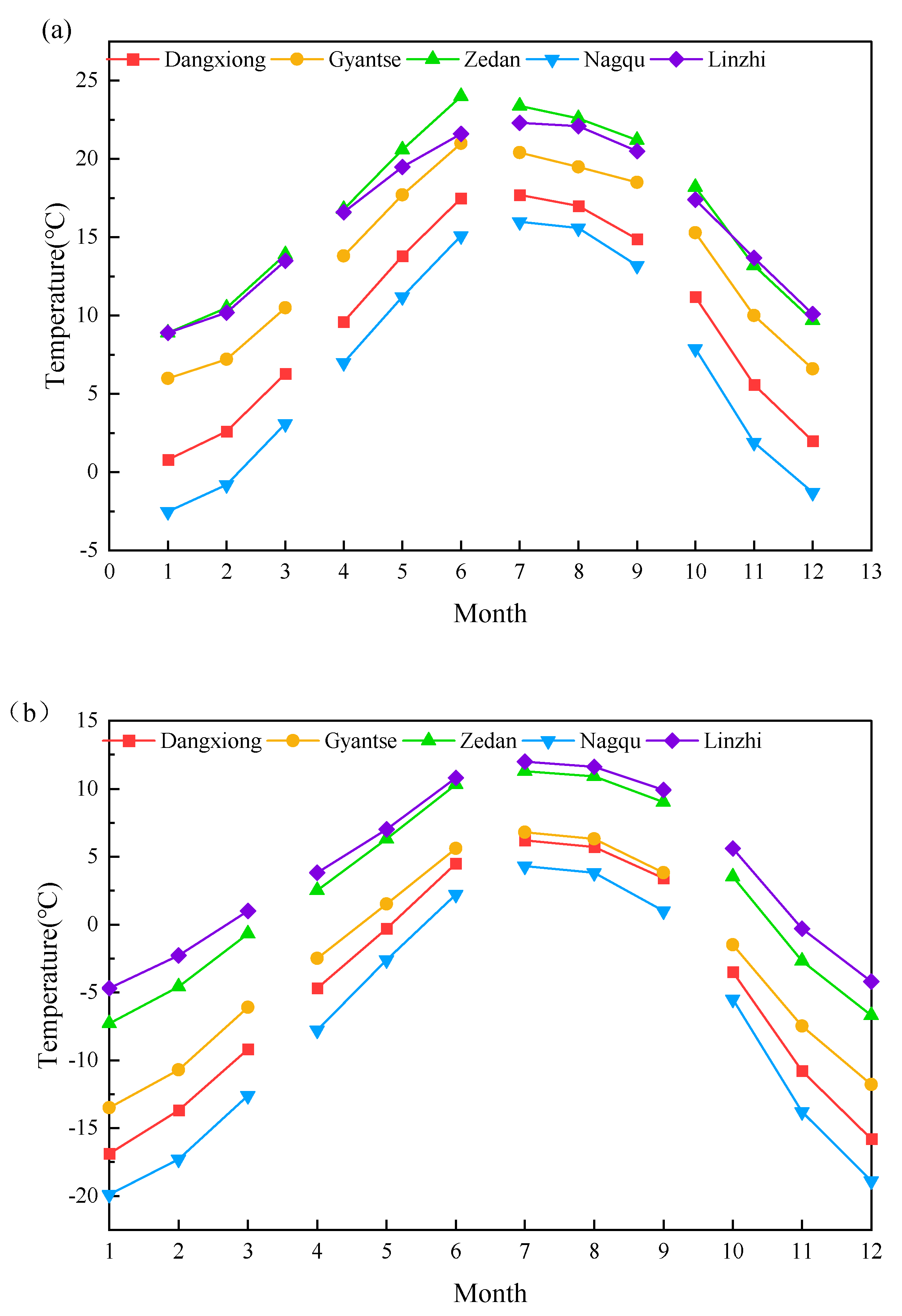
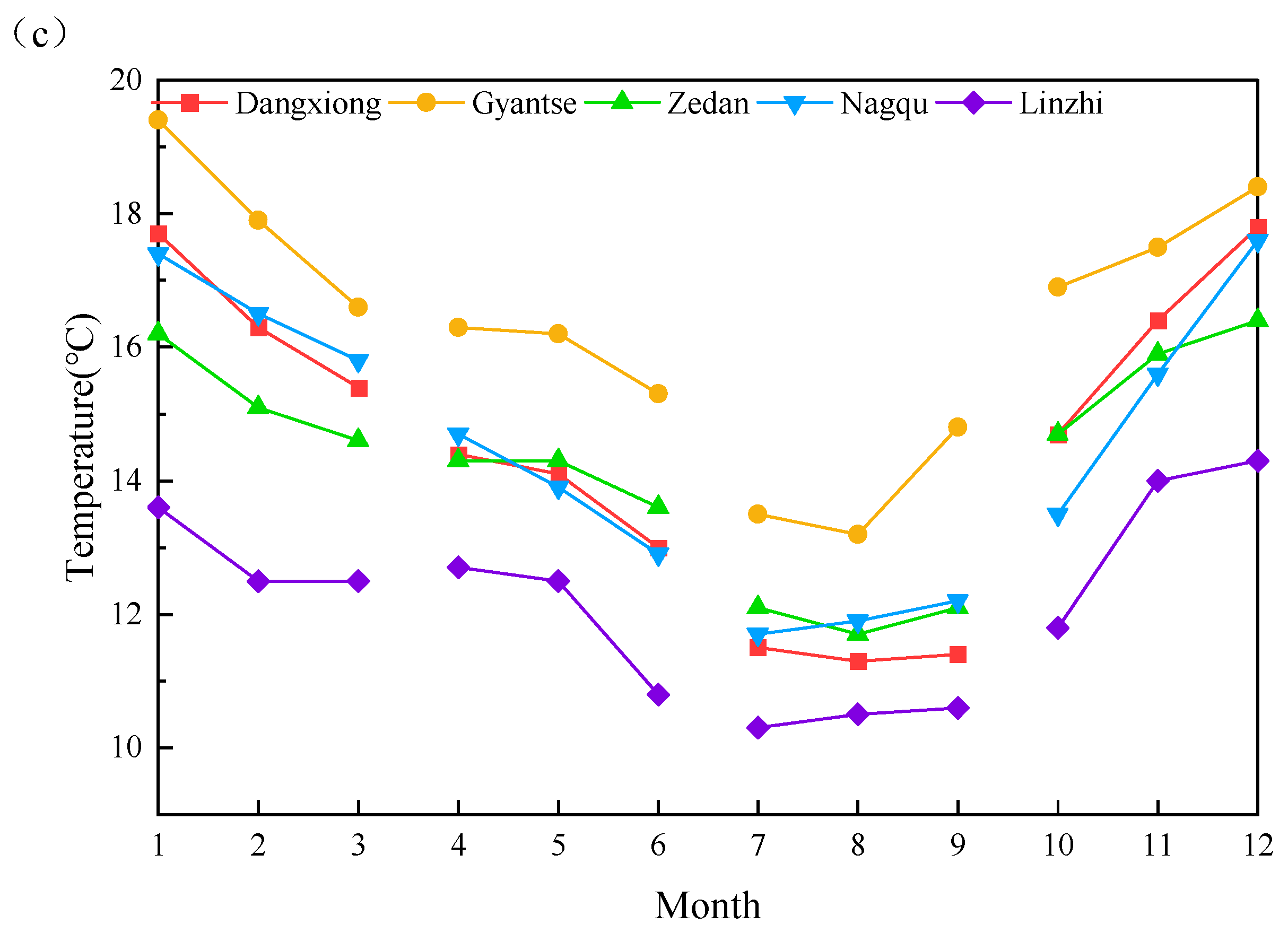
2. Climatic Characteristics of QTP

2.1. Temperature

According to the statistical data of China Meteorological Data Network from 1981 to 2010, the data of five observation stations at different altitudes of Dangxiong, Jiangzi, Naqu, Zedang, and Linzhi were selected to analyze the annual temperature situation (Figure 3). Their geographical location is shown in

Table 1. The geographical location of the five observation stations.

Region	Longitude	Dimensional	Elevation (m)
Dangxiong	90°45′–91°31′ E	29°31′–31°04′ N	4300
Jiangzi	89°06′–90°12′ E	28°30′–29°18′ N	4000
Naqu	83°55′–95°05′ E	29°55′–36°30′ N	4450
Zedang	91°48′ E	29°14′ N	3580
Linzhi	92°09′–98°47′ E	26°52′–30°40′ N	3100

.

The low temperatures months in QTP were mainly in January, February, and December. The mean of the minimum monthly temperature and the mean of the maximum monthly temperature spread both emerged in January. The mean coldest monthly temperature in Nagqu reached −19.9 °C in January and the highest temperature difference in Gyantse was 19.4 °C. In conclusion, the annual temperature in QTP is relatively low, with temperatures below 10 °C most of the time. Thus, asphalt pavements in QTP are very susceptible to shrinkage cracks caused by low temperatures. The extreme temperature difference in winter is large and can even reach more than 30 °C in some areas.

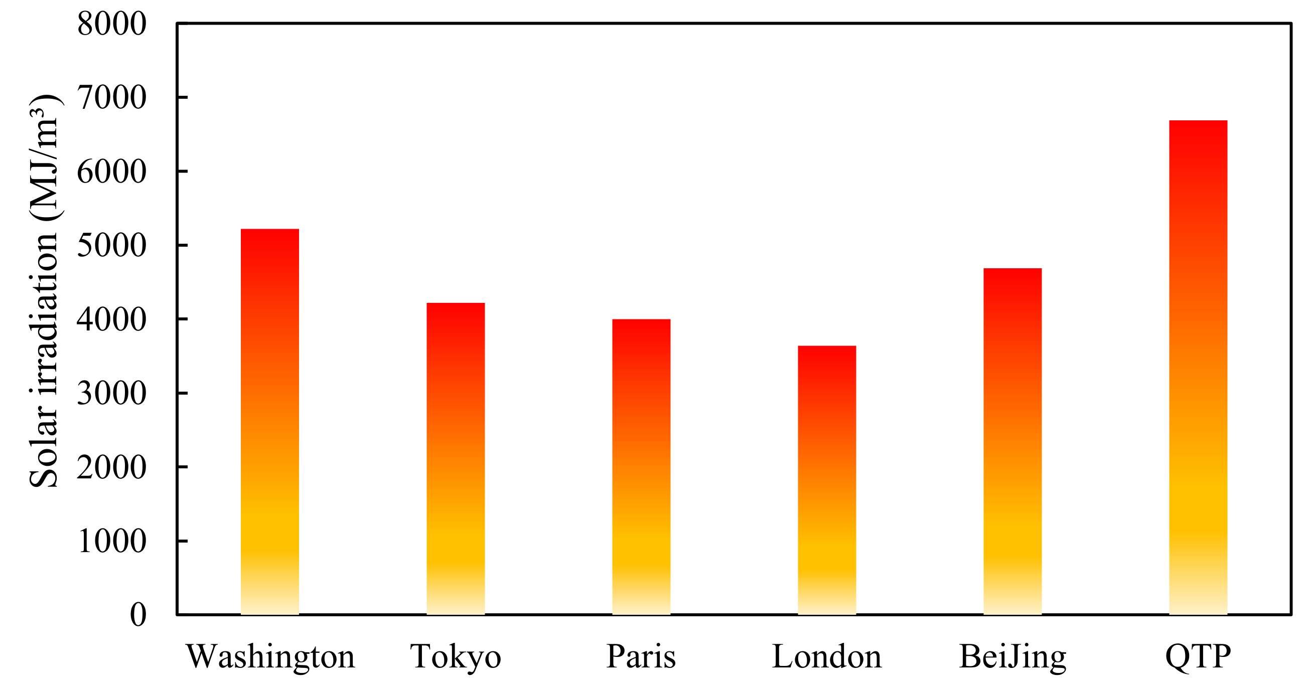
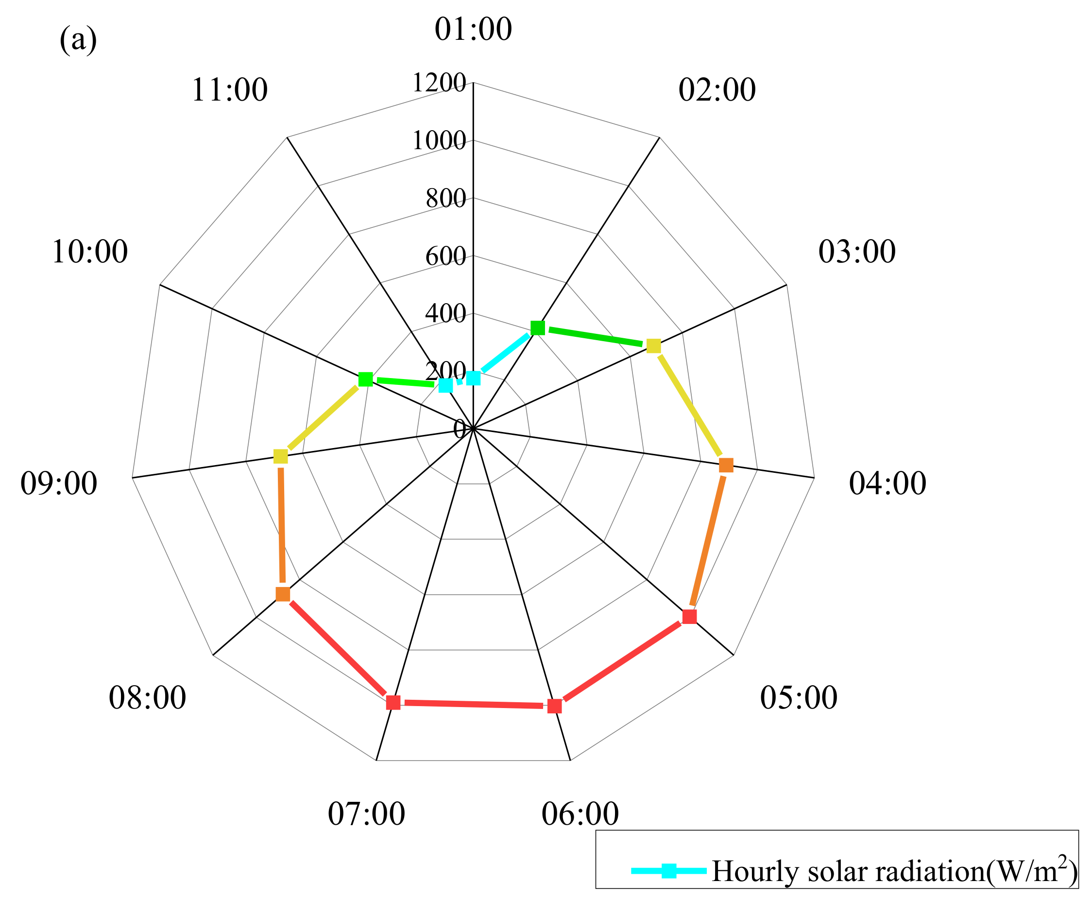
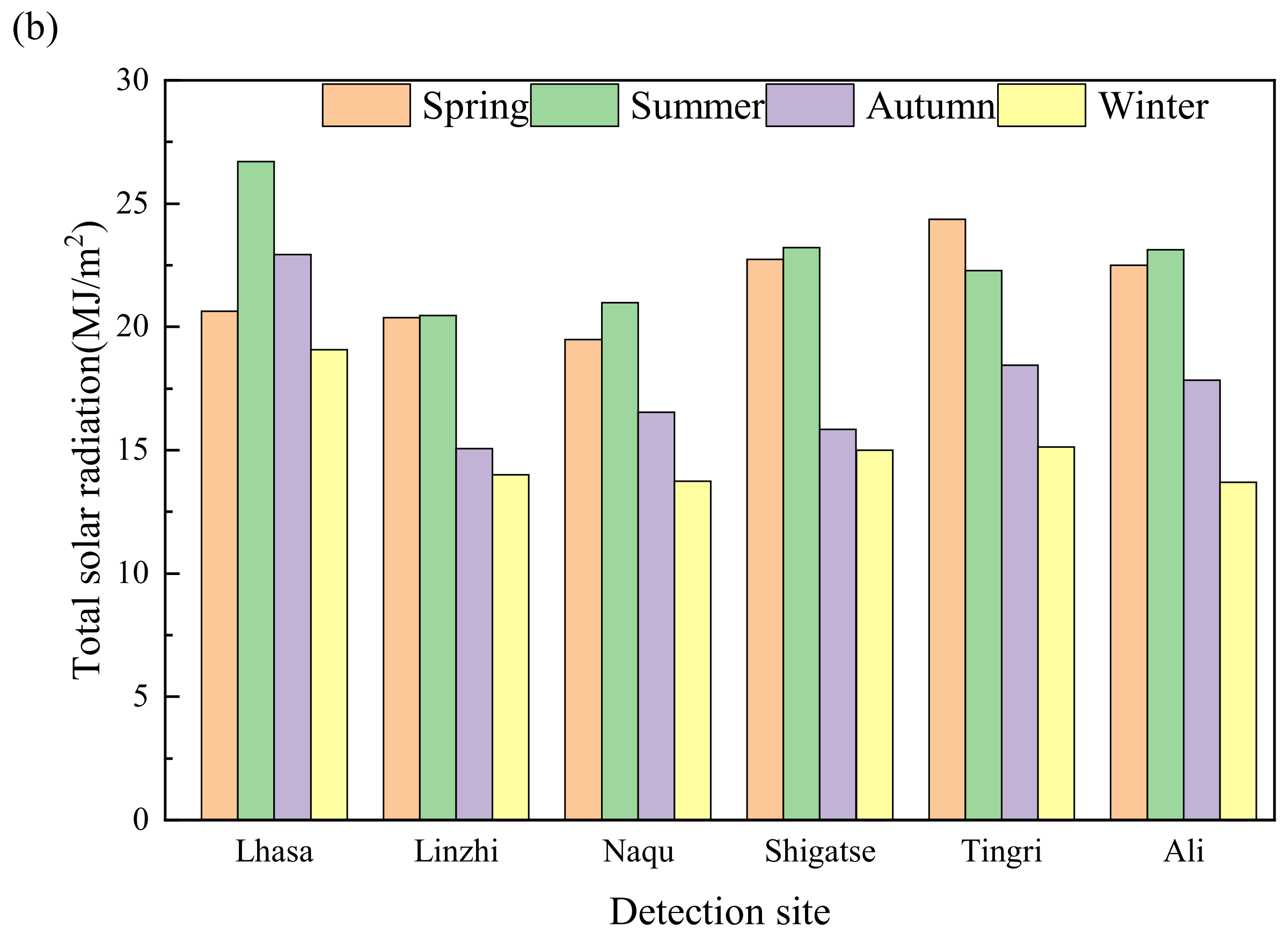
2.2. Solar Radiation

It is apparent from Figure 4 and Figure 5 that QTP is a region of the world with strong solar radiation. The radiation in QTP is strongest in spring and summer and reaches up to 25 MJ/m². Even in winter, the total solar radiation can reach about 15 MJ/m² (Figure 6). The negative climatic conditions in winter can lead to substantial temperature cracks in asphalt pavements in the QTP.

3. Methodology

3.1. Theoretical Equations for Temperature Fields

3.1.1. Differential Equations of Heat Conduction

When the object is a homogeneous isotropic material, and the physical parameters such as material density, specific heat, and thermal conductivity are constants and internal heat sources, the differential equation of heat conduction can be simplified as:

$$\frac{\partial T}{\partial \mathrm{t}}=\alpha (\frac{{\partial }^{2}T}{\partial x^2}+\frac{{\partial }^{2}T}{\partial y^2}+\frac{{\partial }^{2}T}{\partial z^2})$$

(1)

where $\alpha =\lambda /c\rho$ is the heat diffusivity; $\lambda$ is the thermal conductivity, $\mathrm{J}/\left(\mathrm{m}·\mathrm{h}·°\mathrm{C}\right)$; c is the specific heat, $\mathrm{J}/\left(\mathrm{kg}·°\mathrm{C}\right)$; $\rho$ is the density of the material, $\mathrm{kg}/{\mathrm{m}}^3$; and T is the temperature in the pavement.

3.1.2. Boundary Condition

When analyzing the temperature field of the pavement structure, only the temperature change along the thickness direction was considered. The exterior transfer of heat is mostly at the road surface, which transfers heat mainly through thermal radiation and thermal convection.

The heat transferred to the road surface by air convection can be calculated by:

$$q_c=h_c(T_a-T_1\left|{ }_{Z=0}\right.)$$

(2)

The heat transferred to the road surface by radiation can be calculated by:

$$q_r={\alpha }_s\cdot q-q_F$$

(3)

where $T_a$ is the atmospheric temperature, °C; $q$ is the heat transferred to road surface per unit area by solar radiation per unit time; ${\alpha }_s$ is the radiation absorption rate of pavement surface; and $q_F$ is the effective radiation of pavement surface.

(1)

Solar radiation

Solar radiation consists of direct radiation and atmospheric scattering, so solar radiation is impacted by cloud and air transparency. Baber and Middel [28,29] investigated the diurnal variation curve of solar radiation. The diurnal variation curve of solar radiation can be analogous to a sinusoidal half-wave curve. The function of the fitting curve is:

$$q_t=\left\{\begin{array}{ll}0\hfill & 0\le t<12-\frac{c}{2}\hfill \\ q_0\cos m\mathsf{\omega }(t-12)\hfill & 12-\frac{c}{2}\le t\le 12+\frac{c}{2}\hfill \\ 0\hfill & 12+\frac{c}{2}<t\le 24\hfill \end{array}\right.$$

(4)

where $q_0$ is the maximum radiation in a day, which can be calculated by $q_0=0.131mQ$, $m=12/c$; $Q$ is the total solar daily radiation, $J/m^2$; $c$ is the actual effective sunshine time, $h$; and $\omega$ is the angular frequency, which can be calculated by $\omega =2\pi /24\mathrm{rad}$.

To avoid jumping discontinuity points in the calculation of the temperature fields, the above equations can be extended to trigonometric form by means of a Fourier series as follows:

$$q(t)=\frac{{\alpha }_0}{2}+{\displaystyle \sum _{k=1}^{\infty }{\alpha }_k}\cos \frac{k\pi (t-12)}{12}$$

(5)

where ${\alpha }_0=\frac{2q_0}{m\pi }$; ${\alpha }_k=\left\{\begin{array}{ll}\frac{q_0}{\pi }\left[\frac{1}{m+k}\sin (m+k)\frac{\pi }{2m}+\frac{\pi }{2m}\right]\hfill & k=m\hfill \\ \frac{q_0}{\pi }\left[\frac{1}{m+k}\sin (m+k)\frac{\pi }{2m}+\frac{1}{m-k}\sin (m-k)\frac{\pi }{2m}\right]\hfill & k\ne m\hfill \end{array}\right.$;

The intensity of solar radiation absorbed by the road surface can be calculated by:

$$q_s={\alpha }_s\cdot q$$

(6)

where ${\alpha }_s$ is the solar radiation intensity absorption rate of road surface, which was set to 0.90 in this study.

(2)

The change in air temperature

There is a disparity between the time of rise and fall of temperature during one day, with the cooling time being about 4 h longer than the heating time. By using a linear combination of two sinusoidal functions, the practical variation of the temperature process can be well simulated:

$$T_{\mathrm{a}}=\overline{T_a}+T_m[0.96\sin \omega (t-t_0)+0.14\sin 2\omega (t-t_0)]$$

(7)

where $\overline{T_a}$ is the mean daily air temperature, which can be calculated by $\overline{T_a}=1/2(T_a^{\max }+T_a^{\min })$, °C; $T_m$ is the daily temperature variation range, which can be calculated by $T_m=1/2(T_a^{\max }-T_a^{\min })$, °C; $\omega$ is the angular frequency, which can be calculated by $\omega =2\pi /24\mathrm{rad}$, rad; $t_0$ is the primary phase.

The coefficient of heat interaction between the pavement and the atmosphere is primarily governed by the wind speed, which can be expressed by the following equation:

$${\mathrm{h}}_c=3.7v_{\mathrm{w}}+9.4$$

(8)

where $h_c$ is the heat exchange coefficient, $W/(m^2\cdot °\mathrm{C})$; $v_w$ is the daily mean wind speed, m/s.

(3)

Effective radiation of the pavement

The effective radiation of pavement is the difference between the emission of radiation from the pavement and the absorption of inverse atmospheric radiation. The effective radiation of the pavement can be impacted by the internal temperature of the structure and the external meteorological conditions:

$$q_F=\epsilon \sigma [{(T_1\left|{ }_{Z=0}\right.-T_Z)}^4-{(T_a-T_Z)}^4]$$

(9)

where $q_F$ is the effective radiation of road surface, $W/(m^2\cdot °\mathrm{C})$; $\epsilon$ is the road surface emissivity, which can be set to 0.81 in the asphalt pavement; $\sigma$ is the Stefan–Boltzmann constant, which is equal to 56,697 × 10⁻⁸, $W/(m^2\cdot K^4)$; $T_1\left|{ }_{Z=0}\right.$ is the pavement surface temperature, °C; $T_a$ is the air temperature, °C; and $T_Z$ is the absolute zero value, which is equal to −273 (°C).

3.1.3. Solution Equation of Pavement Temperature Field

The temperature field refers to the temperature distribution of each point in an instantaneous object, which is generally a function of space and time coordinates. In the rectangular coordinate system, the temperature field can be expressed as:

$$T=f(x,y,z,t)$$

(10)

The heat conduction differential equation of pavement structure can be expressed as:

$$\frac{\partial T_i(z,t)}{\partial t}={\alpha }_i\frac{{\partial }^2{T}_{\mathrm{i}}(z,t)}{\partial z^2}$$

(11)

When the interlayer structure is good without thermal resistance, the interlayer interface satisfies:

$$T_i(z,t)\left|{ }_{z=z_i}=T_{i+1}(z,t)\left|{ }_{z=z_i}\right.\right.$$

(12)

$${\lambda }_i\frac{\partial T_i(z,t)}{\partial t}\left|{ }_{z=z_i}\right.={\lambda }_{i+1}\frac{{\partial }^2{T}_{\mathrm{i}+1}(z,t)}{\partial z}\left|{ }_{z=z_i}\right.$$

(13)

where ${\alpha }_i$, ${\lambda }_i$, and $h_i$ represent the thermal conductivity, thermal conductivity, and structural layer thickness of the first layer pavement structure layer, respectively.

3.2. Basic Assumption

In the establishment of the temperature field model, the following assumptions were made to facilitate the analysis and calculation of the problem:

(1)

The pavement surface, subgrade, bedding layer, and soil base are considered homogeneous, isotropic, and elastic materials.

(2)

The layers of the pavement structure are tightly connected to each other and the stresses, displacement, and heat fluxes vary continuously among the layers.

(3)

The inhomogeneity of the lateral distribution of the pavement temperature field is neglected.

(4)

The transfer of heat flow is assumed to be one-dimensional conduction perpendicular to the pavement.

(5)

The parameters are considered not to vary with temperature, except for the relevant parameters mentioned in the paper.

(6)

Due to the asphalt mixture’s inhomogeneity and discontinuities between layers could have an effect on the localized calculation results of the temperature field of asphalt pavement, but it has little effect on the overall calculation results. If further accurate local temperature field calculations are desired, a 3D temperature field model that takes into account the inhomogeneities and discontinuities can be built. The calculation accuracy of the model used in this paper has met the needs of the study.

3.3. Structure and Parameters of the Pavement

This section lists the various parameters used for modeling. The thermophysical parameters of the pavement structure and pavement materials according to the typical sections of the QTP are listed in

Table 2. Thermodynamic parameters of materials.

Structural Layer	Above Layer AC-13	Lower Layer AC-20	Base Cement Stabilized Macadam	Cushion Graded Gravel	Soil
Thickness (cm)	4	5	20	20
Thermal conductivity $(\mathrm{J}/\left(\mathrm{m}\cdot \mathrm{h}\cdot °\mathrm{C}\right))$	4200	4000	5400	5200	5400
Density $(\mathrm{kg}/{\mathrm{m}}^3)$	2400	2500	2100	2000	1800
Specific heat $(\mathrm{J}/(\mathrm{kg}\cdot °\mathrm{C}))$	950	900	900	950	1000
Solar radiation absorptivity	0.9
Road surface reflectance	0.81
Absolute zero (°C)	−273
Stefan–Boltzmann constant $(\mathrm{J}/(\mathrm{h}\cdot {\mathrm{m}}^2\cdot {\mathrm{K}}^4))$	2.041 × 10−4

. The elastic parameters and temperature shrinkage coefficients of the materials used in this study are given in

Table 3. Elastic parameters of materials.

Structural Layer	Material Type	Temperature (°C)	Elastic Modulus (MPa)	Poisson’s Ratio
Above layer	AC-13	10	900	0.3
		0	1400	0.3
		−10	4500	0.25
		−20	9000	0.25
		−30	14,000	0.25
Lower layer	AC-20	10	1000	0.3
		0	1200	0.3
		−10	4200	0.25

and

Table 4. Temperature shrinkage coefficient.

Material Type		Temperature Shrinkage Coefficient at Different Temperatures (×10−5)
		0 °C	−10 °C	−20 °C	−30 °C
Asphalt mixture	AC-13	2.5	2.2	1.9	1.6
	AC-20	2.5	2.2	1.9	1.6
Cement stabilized macadam		0.98
Graded gravel		0.5
Soil		50

.

According to the meteorological data, this study was conducted in January after excluding the effect of cold waves. The meteorological parameters of the pavement structure of QTP under the periodic temperature of the cold season are shown in

Table 5. The temperature for 24 h on behalf of the day in winter (January).

Time (h)	0	1	2	3	4	5	6	7	8	9	10	11
Temperature (°C)	−9.1	−10.1	−11.1	−12.1	−12.9	−13.5	−13.7	−13.4	−12.7	−11.5	−9.9	−8.2
Time (h)	12	13	14	15	16	17	18	19	20	21	22	23
Temperature (°C)	−6.4	−4.8	−3.6	−2.9	−2.6	−2.8	−3.4	−4.2	−5.2	−6.2	−7.2	−8.2

. The total daily solar radiation is 15.1 MJ/m²; the daily mean wind speed is 2.0 m/s; and the effective duration of sunshine is 7.5 h.

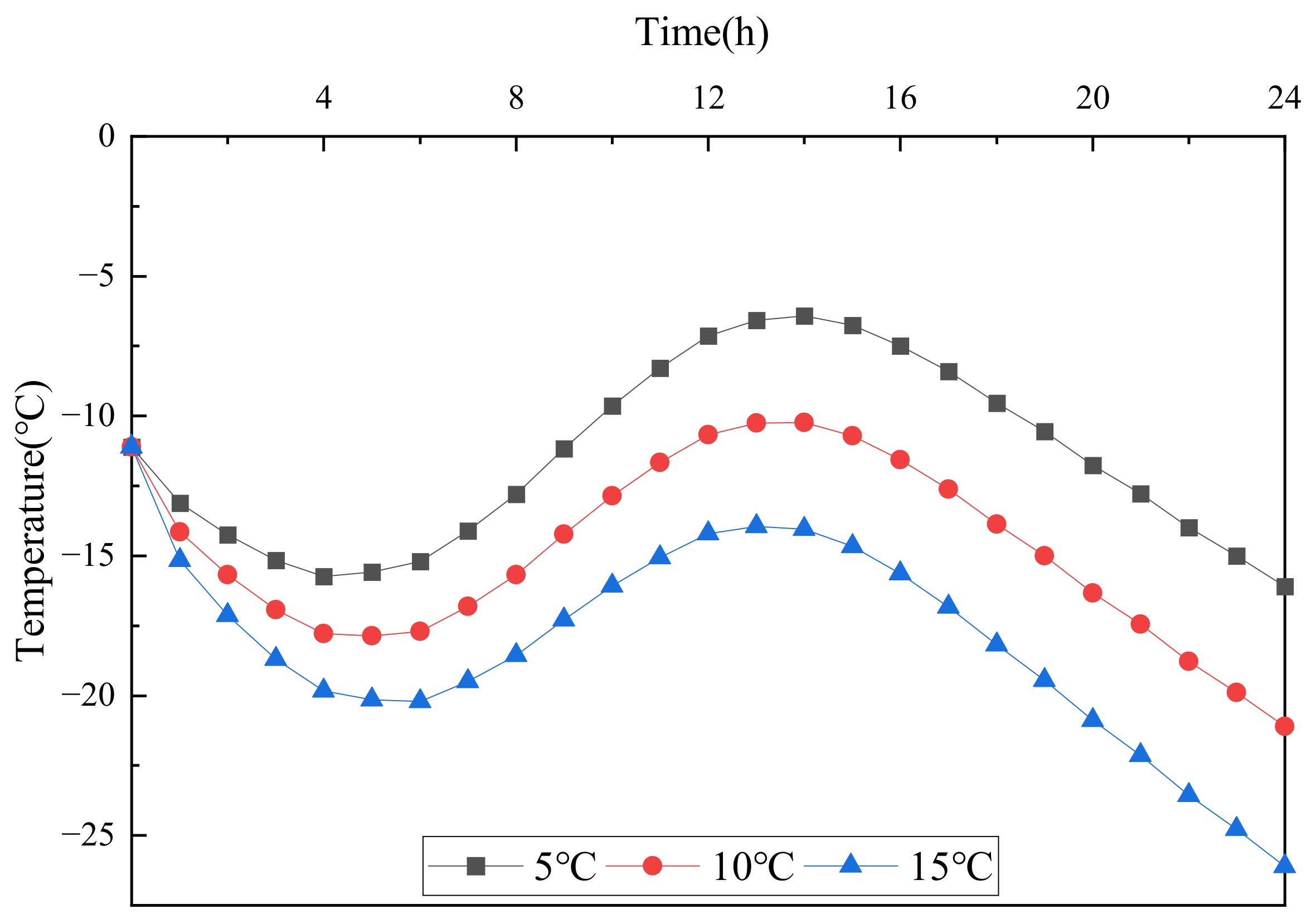
3.4. Initial Temperature Field of Asphalt Pavement

The initial temperature field of the pavement structure is ascertained to enhance the simulation reliability of the temperature field [30].

The calculation formula of pavement temperature can be calculated by:

$$T_0=64.9e^{0.014T_{\mathrm{a}1}}+e^{1.16Q_4}-66.4$$

(14)

where $T_0$ is the pavement surface temperature, °C; $T_{a1}$ is the atmospheric temperature an hour ago, °C; and $Q_4$ is the cumulative solar radiation intensity in the first 4 h, $\mathrm{kW}/{\mathrm{m}}^2$.

The pavement temperature at different depths can be calculated by:

$$T_h=T_0+(7.01e^{-0.07h}-7.01)\times \sin (0.011h-0.316t-0.659)-0.003h\times T_0$$

(15)

where $T_h$ is the temperature at different depths of the pavement, °C; $T_0$ is the pavement surface temperature, °C; and $h$ is the depth from road surface, cm.

3.5. Determination of Cooling Range

The cold wave in QTP often occurs in January, and the cooling amplitude of the cold wave ranges from a few degrees to a dozen degrees. Therefore, in order to make the simulated cooling situation closer to the actual situation, the temperature stresses in the pavement structure under different cooling amplitudes are calculated by considering the cooling amplitude values of 5 °C, 10 °C, and 15 °C, respectively.

After studying and analyzing the pavement structure under low-temperature conditions [31], it was obtained that in excluding the cold wave cooling process, the following equation can be fitted:

$$\Delta t_a=\Delta t_{Ma}{\left(t^{\prime }/{t^{\prime }}_{Ma}\right)}^{n_a}$$

(16)

where $\Delta t_{Ma}$ is the maximum amount of cooling; $t^{\prime }$ is the time that from the beginning of cooling is zero point, $0\le t^{\prime }\le {t^{\prime }}_{Ma}$; ${t^{\prime }}_{Ma}$ is the total time of cooling process; and $n_a$ is the fitting coefficient, set to 0.5.

The cooling process within 24 h without considering the daily temperature fluctuation is shown in Figure 7. It can be seen from the figure that the temperature drop rate gradually decreases during the day. The actual ambient temperature of the road surface is the result of the superposition of the daily temperature change and the cooling process. Therefore, the 24 h actual temperature of the pavement is the sum of the daily temperature in Table 5 and the temperature in Figure 7. The actual temperature of the road surface after the superposition of the cooling process is shown in Figure 8.

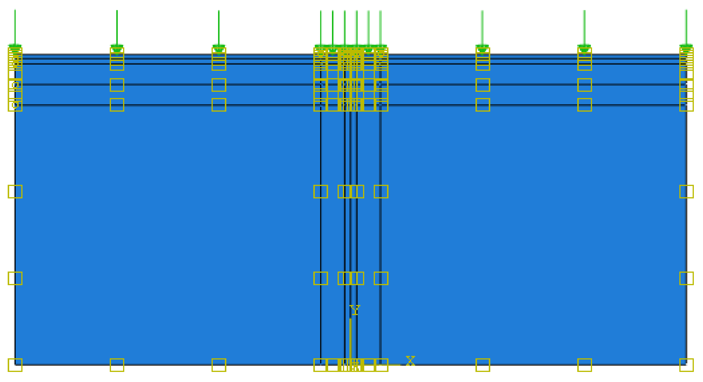
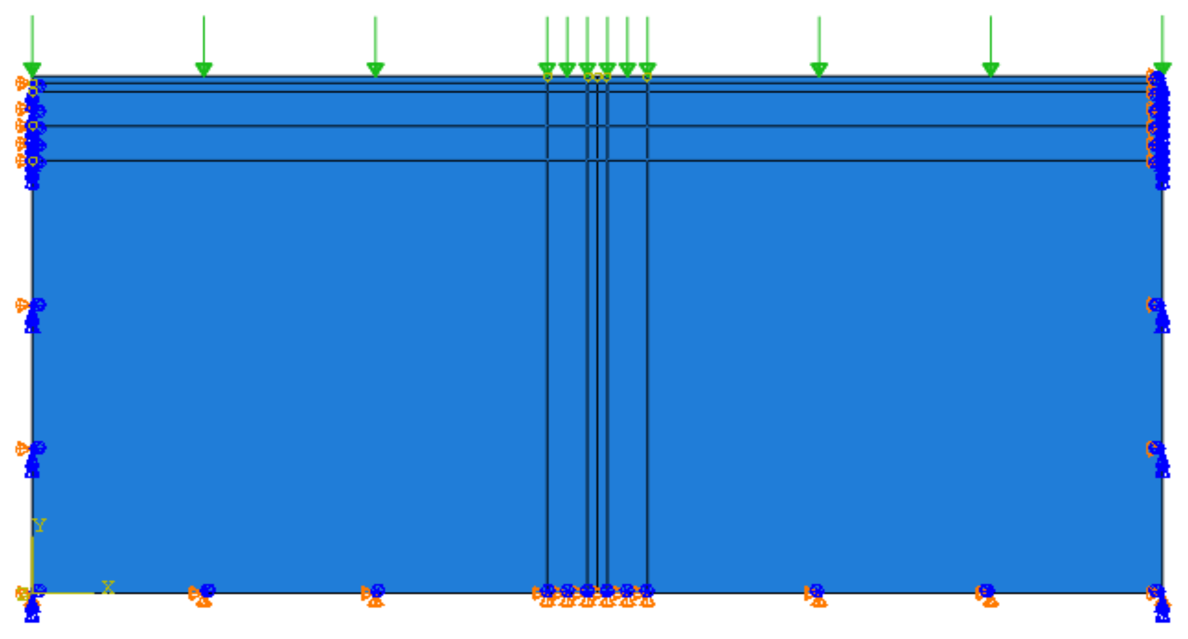
3.6. Temperature Field Model

The pavement of the normal national and provincial roads in QTP is typically 6 m wide. Accordingly, the length of the module in this study was set to 6 m and the thickness was set to 3 m. The model of the temperature field is shown in Figure 9.

3.7. Thermal Stress Model

In ABAQUS, the elastic modulus, Poisson’s ratio, and temperature shrinkage coefficient in the material properties were set as elastic parameters that vary with temperature. The boundary conditions were defined as XSYMM for the left and right and ZASYMM for the bottom. The results of the temperature field were imported into the thermal stress calculation model and the grid division was consistent with the temperature field model. The element type was set to a four-node temperature surface strain quadrilateral reduced integral element (CPE4RT). The thermal stress model is displayed in Figure 10.

4. Result and Discussion

4.1. Verification of Numerical Modeling

For typical sections of the QTP, the calculated temperature data and observed road surface data are shown in Figure 11.

Due to the continuous and stable temperature of numerical simulation, the measured temperature is severely affected by the environment, resulting in discontinuous and large fluctuations in the data. The simulated temperature data are not identical to the measured data. However, they are similar to each other, and more importantly, they have similar variation trends. The mean value of the residuals between the finite element simulated and measured values of the road surface temperature is −0.27, and the standard deviation of the residuals is 0.49, which shows that the simulation accuracy is good. The validity of the finite element model for the response of pavement temperature field and thermal stress is proved.

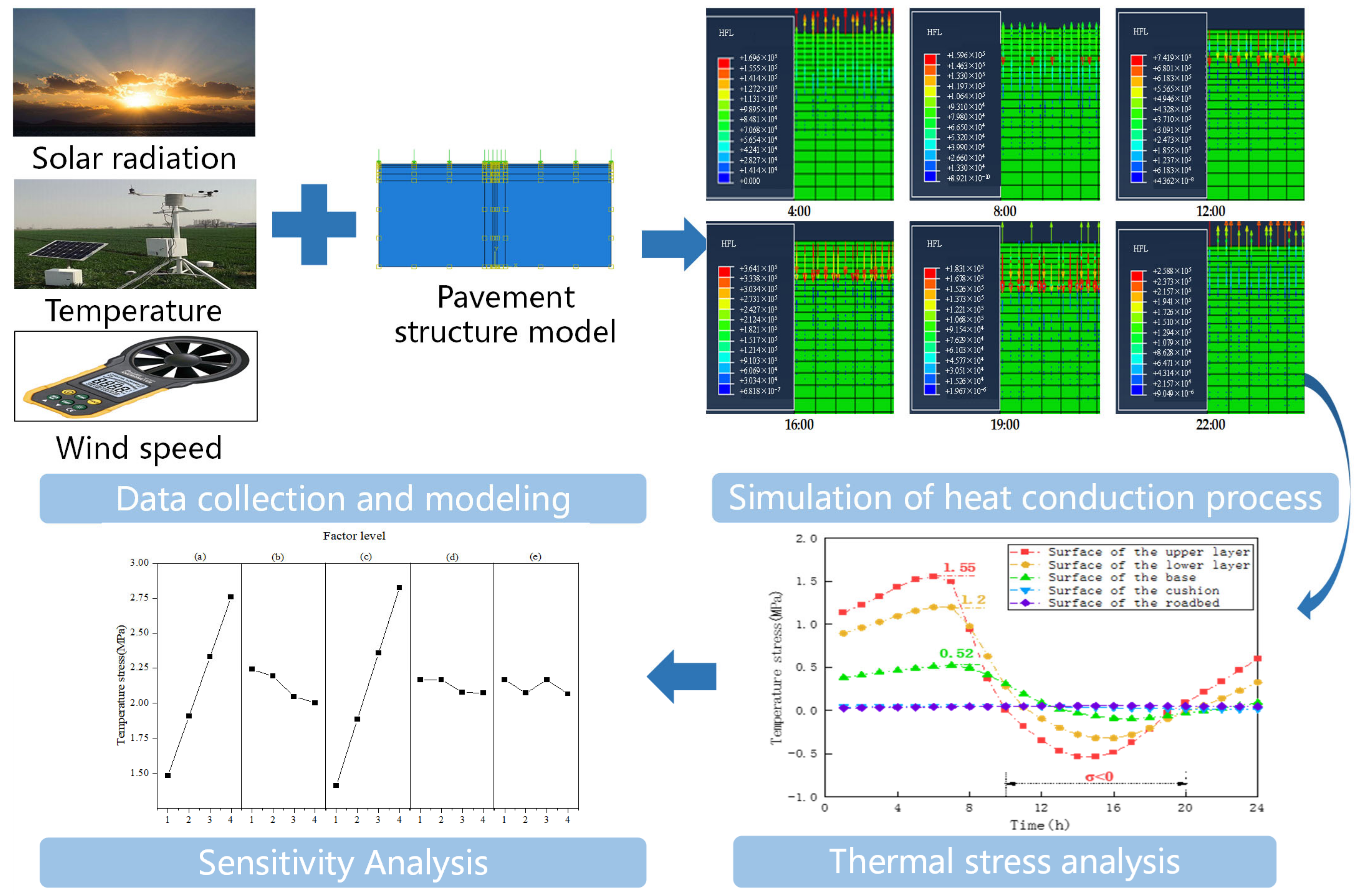
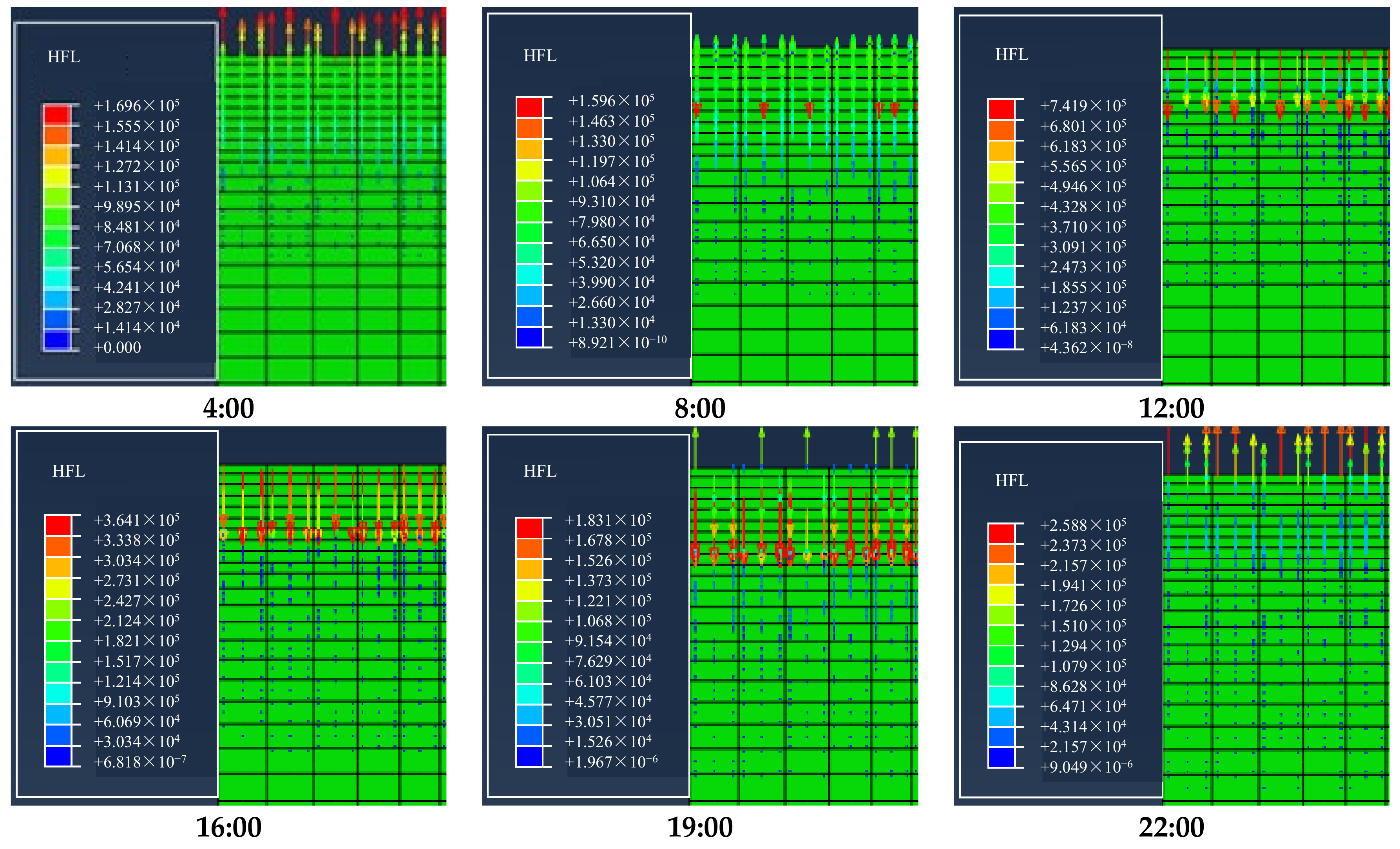
4.2. Variation of the Heat Flow Vector

Figure 12 shows the variation of the heat flux vector of the pavement structure during the day.

As can be seen in Figure 12, towards the evening, the pavement can release heat to the surroundings due to the weakening of solar radiation. Consequently, the temperature of the pavement structure can gradually decrease. However, due to the solar radiation during the day, the pavement can attract the heat transferred from the atmosphere and the temperature of the pavement structure can grow gradually. Repeated heating and cooling can lead to the accumulation of fatigue damage in the pavement structure. Eventually, temperature cracks are generated.

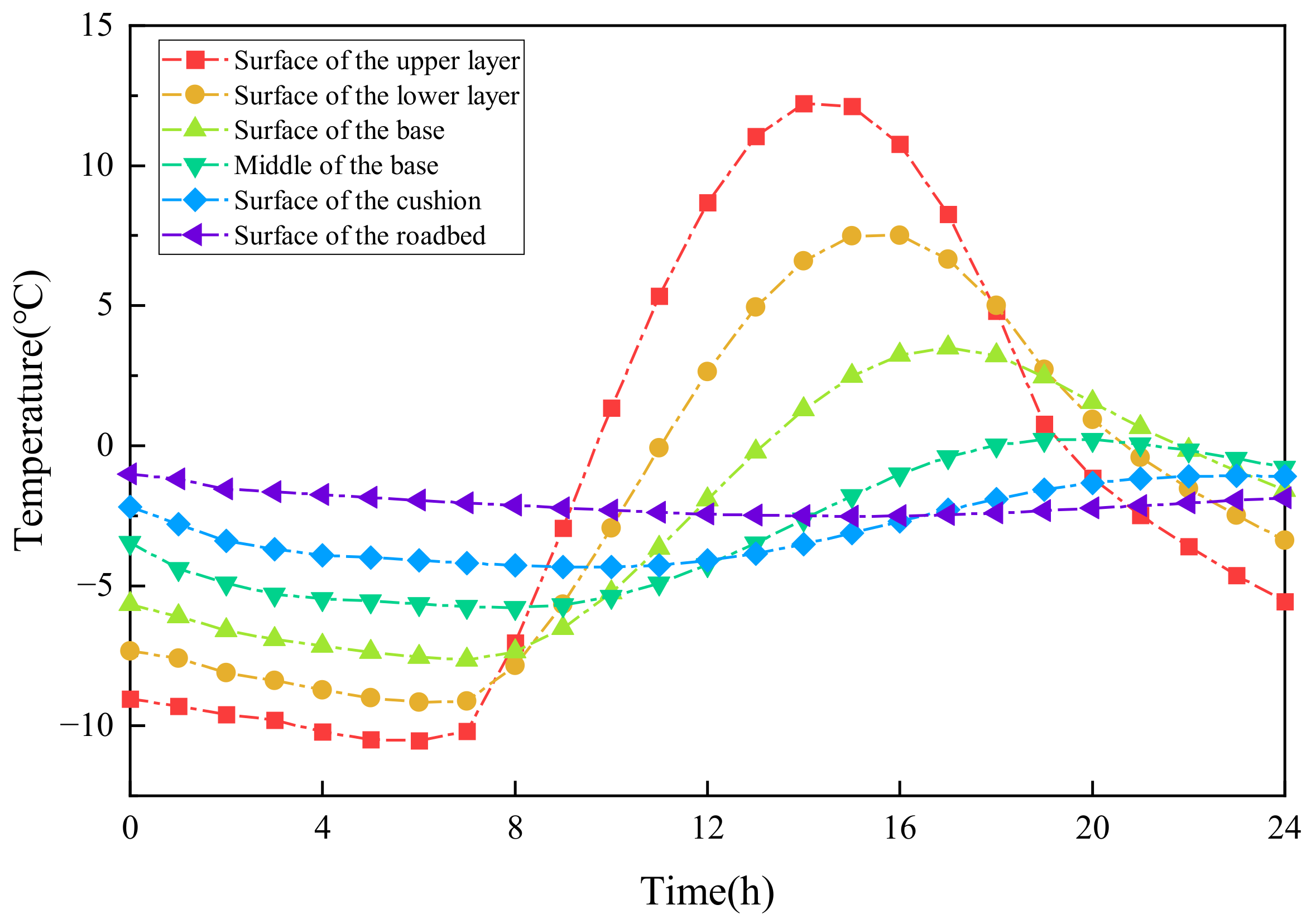
4.3. Variation of Pavement Temperature

The temperature changes in the pavement structure at different times of the day are displayed in Figure 13, from which it can be revealed that the maximum temperature of the asphalt pavement in the QTP is about 12 °C at 15:00, while the maximum temperature of the representative day in January is −2.6 °C, which is due to the strong solar radiation in the QTP. The maximum pavement temperature usually appears 1–2 h after the maximum solar radiation and the maximum solar radiation in the QTP is at 14:00 in winter, so the simulation results are consistent with the pavement temperature. The lowest pavement temperature occurs around 6:00, which is about −11 °C. The temperature difference between day and night in winter causes a large change in pavement temperature. In the long term, the pavement is vulnerable to fatigue cracks.

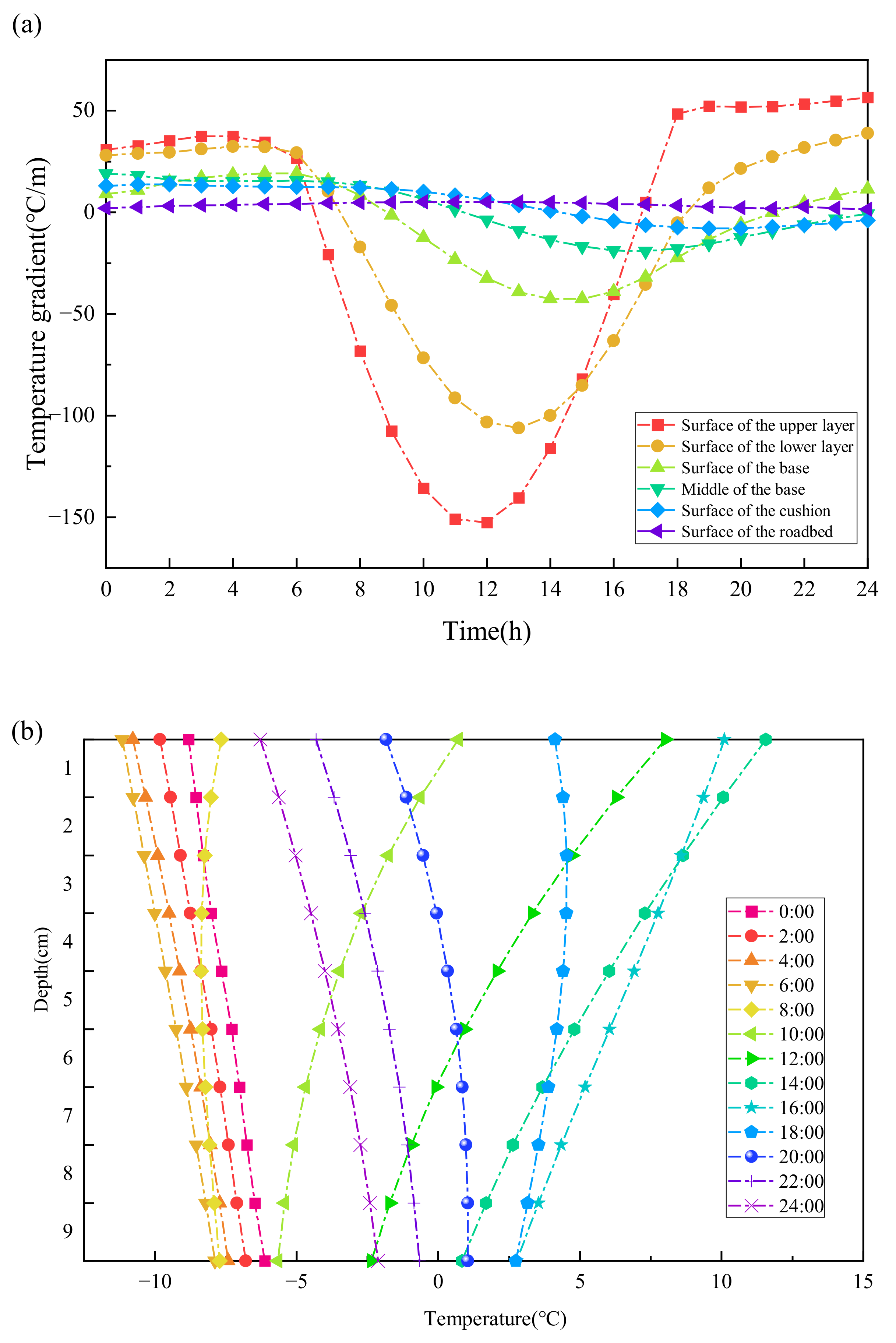
4.4. Variation of Temperature Gradient

The variation of the pavement temperature field with depth in the QTP is shown in Figure 14.

From Figure 14a, it can be concluded that the surface layer is significantly influenced by temperature and radiation. The extremes of positive and negative temperature gradients on the pavement reach 52.2 °C/m and −152.6 °C/m, respectively. The negative temperature gradient changes faster due to the influence of radiation during the daytime, and the large changes in the temperature gradient can lead to vertical fatigue damage to the pavement structure. It can be noticed from Figure 14b that the temperature field of the surface layer is complicated. At 12:00 and 14:00, the temperature difference between the surface layer and the bottom of the lower layer reaches more than 10 °C. Solar radiation is the main factor contributing to this phenomenon, which can be ameliorated by solar heat reflective coating.

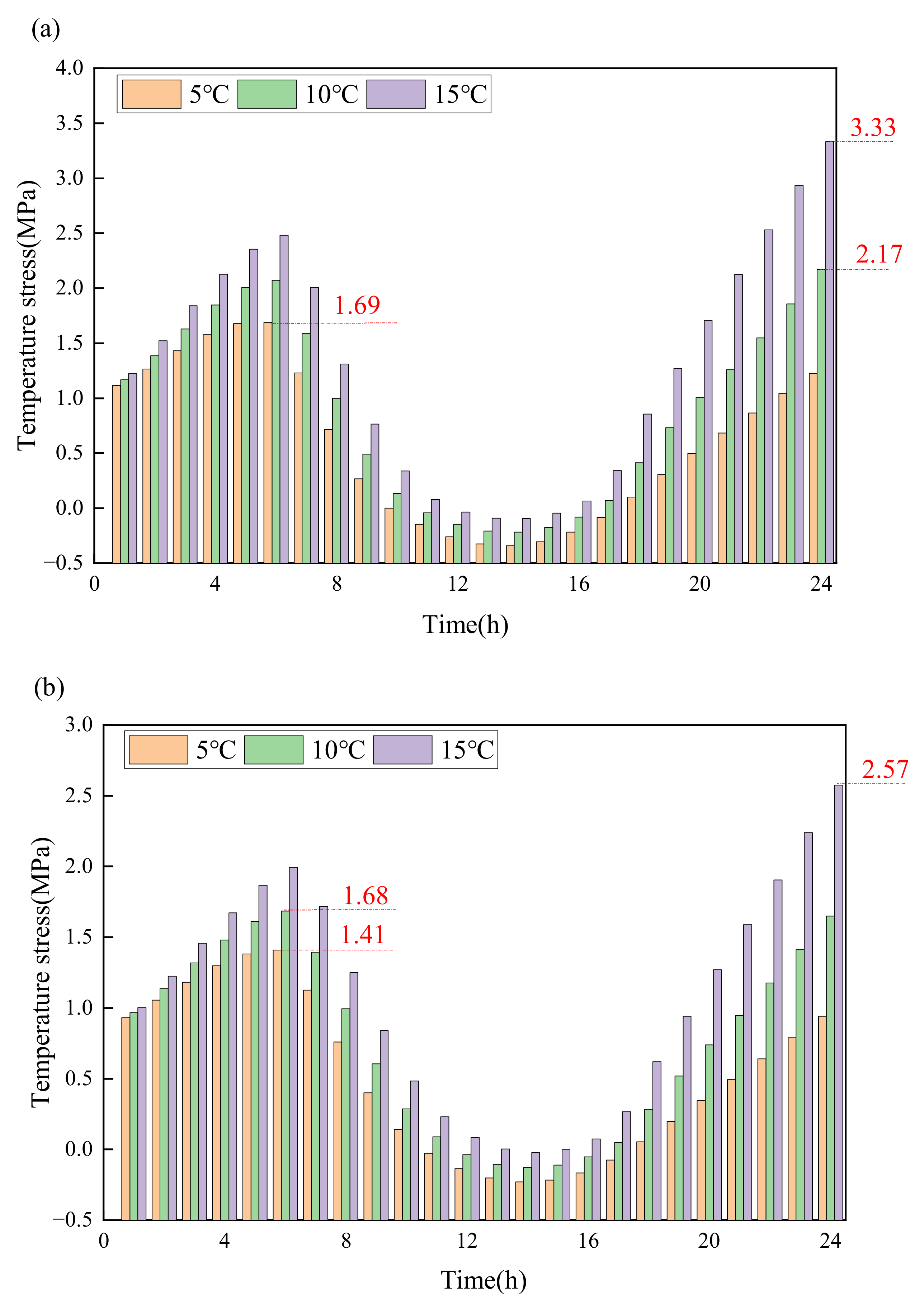
4.5. Analysis of Thermal Stress in One Day

The pavement temperature field is channeled into the thermal stress model and the thermal stresses of the corresponding structural layers are exported through the field variables. The variation of daily thermal stresses is shown in Figure 15.

From Figure 15a, it can be noted that the maximum peak of thermal stress in the pavement occurs at 6:00 a.m., which is 1.55 MPa. The greatest thermal stress on the lower surface is 1.2 Mpa, which occurs at 7:00 a.m. Also, from the figure, it can be revealed that the tensile stress period in the pavement under the role of low temperature is from 20:00 to 10:00, and fatigue cracks can occur in the long-term tensile state.

As can be seen in Figure 15b, the stresses in the pavement gradually decrease along the depth. There is a certain hysteresis in the change in thermal stress between the upper and lower layers. The reason for this is that the modulus and temperature shrinkage coefficient of the upper and lower layers are temperature dependent, and the thermal load has a certain response time.

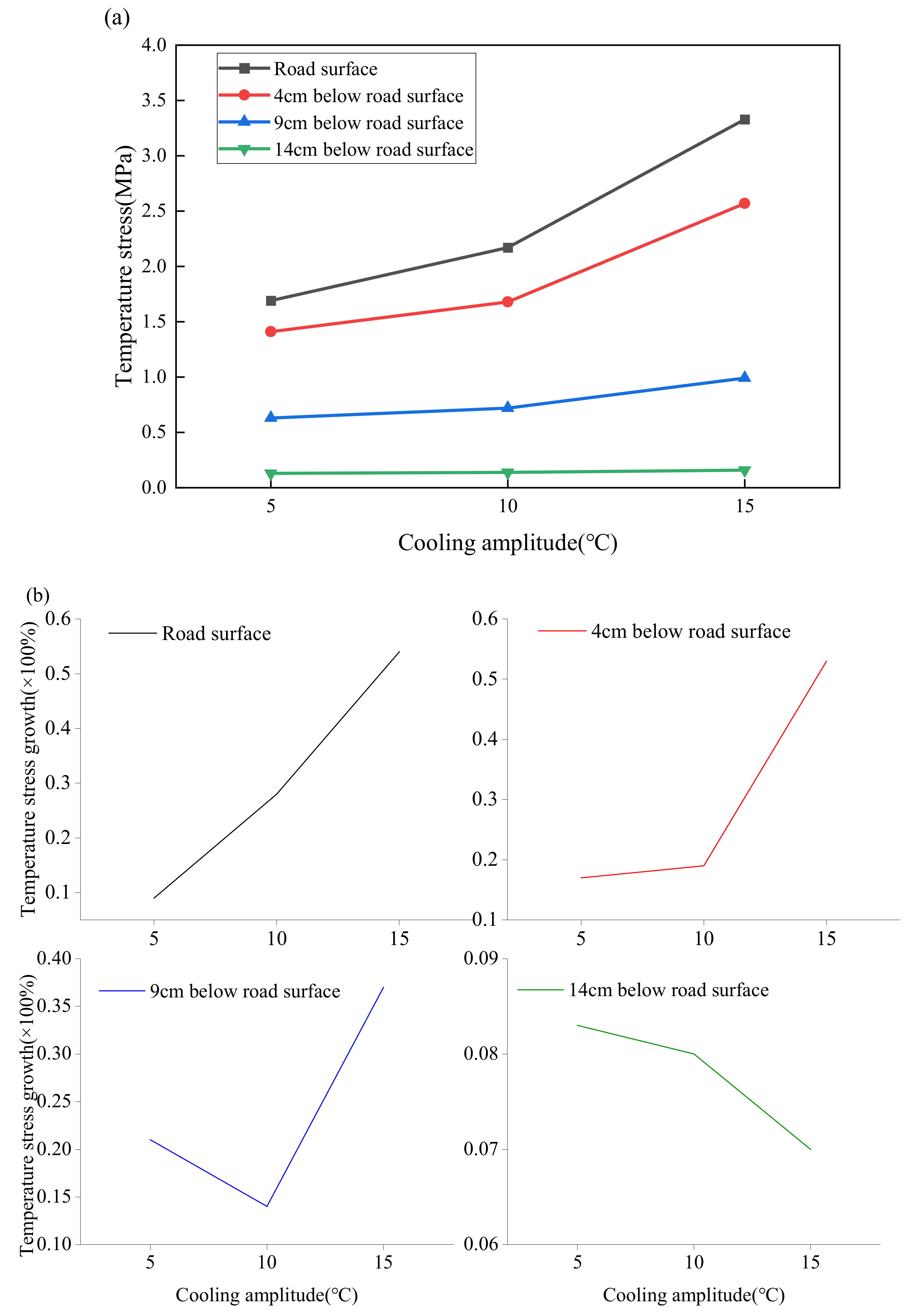
4.6. Analysis of Thermal Stress in Cold Wave

In the study, the temperature conditions of 5 °C, 10 °C, and 15 °C of cooling were selected to simulate the thermal stress changes in asphalt pavement under different cooling amplitudes. And it was selected 0 cm, 4 cm, 9 cm, and 14 cm below the pavement for the analysis. The thermal stress distribution of the pavement structure layer at different depths is illustrated in Figure 16.

It can be revealed from Figure 16 that the greater the cooling amplitude, the greater the thermal stress generated in the pavement and the longer the pavement is in a tensile state. When the cooling amplitude is 15 °C, the maximum thermal stress of the pavement reaches 3.33 MPa, which easily exceeds the splitting tensile strength of the AC-13 asphalt mixture. It leads to the low-temperature shrinkage cracking of the pavement.

The asphalt pavement surface layer is most obviously subjected to cooling as seen in Figure 17. When the cooling range of the pavement reaches 15 °C, the maximum thermal stress reaches 3.33 MPa and the thermal stress increases linearly with a maximum increase of 53%. The maximum thermal stress also reaches 2.57 MPa when the cooling range of the lower pavement reaches 15 °C, and the greatest percentage increase in the thermal stress also reaches more than 50%. When the temperature is quite low, the modulus of asphalt concrete increases rapidly, showing brittle and stiff characteristics. Due to the changeable weather of the QTP, under the combined influence of various unfavorable weather factors, the thermal stress is very likely to exceed the tensile strength of the asphalt mixture, resulting in pavement cracking.

4.7. Parameter Sensitivity Analysis

A sensitivity analysis of the factors influencing surface stress was performed in this research by designing an orthogonal test. Then, the main factors affecting the surface thermal stresses were found. It can offer a basis for the design of pavement structures against cracking.

4.7.1. Orthogonal Experimental Design

To analyze the influencing factors of the shear strength, orthogonal tests were utilized. Orthogonal tests are an experimental design method that evaluates the effects of multiple factors and levels on a single target variable [32]. Four influencing factors of surface modulus, surface thickness, surface temperature shrinkage coefficient, and base modulus were selected, respectively. They are highly effective in evaluating the influence of multiple factors on the target variable and identifying the optimal level for each factor. The experimental factor levels and design for orthogonal tests are presented in

Table 6. Orthogonal analysis factor level table.

Factor/Level	Surface Modulus (MPa)	Surface Thickness (cm)	Surface Temperature Shrinkage Coefficient (10−5/°C)	Base Modulus (MPa)
1	3500	9	1.5	1200
2	4500	12	2	1500
3	5500	15	2.5	1800
4	6500	18	3	2100

and

Table 7. Thermal stress calculation results.

Test Serial Number	Surface Modulus (MPa)	Surface Thickness (cm)	Surface Temperature Shrinkage Coefficient (10−5/°C)	Base Modulus (MPa)	Blank Column	Thermal Stress (MPa)
1	1 (3500)	1 (9)	1 (1.5)	1 (1200)	1	0.99
2	1	2 (12)	2 (2.0)	2 (1500)	2	1.32
3	1	3 (15)	3 (2.5)	3 (1800)	3	1.65
4	1	4 (18)	4 (3.0)	4 (2100)	4	1.98
5	2 (4500)	1	2	3	4	1.70
6	2	2	1	4	3	1.27
7	2	3	4	1	2	2.54
8	2	4	3	2	1	2.12
9	3 (5500)	1	3	4	2	2.59
10	3	2	4	3	1	3.11
11	3	3	1	2	4	1.55
12	3	4	2	1	3	2.07
13	4 (6500)	1	4	2	3	3.68
14	4	2	3	1	4	3.06
15	4	3	2	4	1	2.45
16	4	4	1	3	2	1.84

respectively. Each factor takes four levels, and the values of each factor and level are shown in Table 6.

The orthogonal test was performed with five factors and four levels. L16(45) was chosen, and the fifth column was blank. The orthogonal test table was generated by Minitab software. Altogether, 16 tests were calculated. The results of the maximum thermal stress calculation are listed in Table 7.

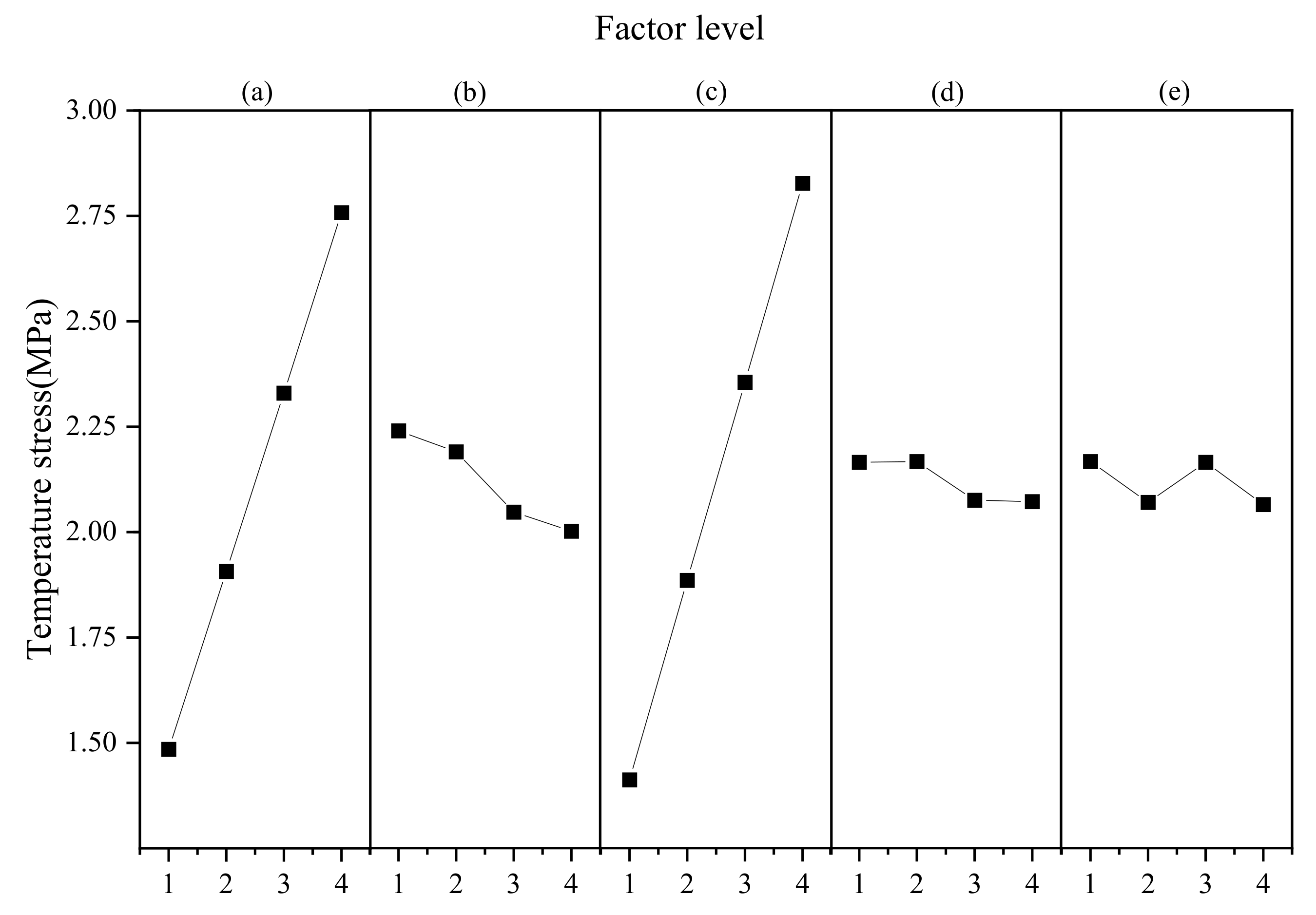
4.7.2. Extremum Difference Analysis

In this study, Minitab was used to analyze the maximum thermal stress of the pavement at each factor level. The results are illustrated in

Table 8. Range analysis results of the orthogonal test.

Level	Surface Modulus	Surface Thickness	Surface Temperature Shrinkage Coefficient	Base Modulus
1	1.485	2.240	1.412	2.165
2	1.907	2.190	1.885	2.167
3	2.330	2.047	2.355	2.075
4	2.758	2.002	2.827	2.072
Extreme difference	1.273	0.237	1.415	0.095

.

From the results, it can be concluded that the surface modulus and surface temperature shrinkage coefficient have the greatest effect on the thermal stress of the pavement. The order of influence of various factors on thermal stresses is surface temperature shrinkage coefficient > surface modulus > surface thickness > base modulus. Consequently, the material parameters of the pavement structure should be mainly considered in the design of the pavement structure in the QTP to ensure the crack resistance of the pavement structure. The mean response of each factor at different levels is shown in Figure 18.

Figure 18 indicates that reducing the modulus and temperature shrinkage coefficient of the surface layer can effectively diminish the thermal stress of the pavement. Hence, materials with small modulus and temperature shrinkage coefficient should be selected as much as possible in the design of pavement structure, and the thickness of the surface layer can be enlarged appropriately. The optimal pavement structure combination obtained by polarization is listed in

Table 9. Optimum combination of the pavement structure.

Surface Modulus (MPa)	Surface Thickness (cm)	Surface Temperature Shrinkage Coefficient (10−5/°C)	Base Modulus (MPa)	Base Thickness (cm)
3500	18	1.5	2100	20

.

4.7.3. Analysis of Variance

Variance analysis results of the orthogonal test are shown in

Table 10. Thermal stress variance analysis.

Project	Surface Modulus	Surface Thickness	Surface Temperature Shrinkage Coefficient	Base Modulus
Degree of freedom (DF)	3	3	3	3
The sum of squares deviation from the mean (MS)	3.596	0.153	4.446	0.034
Mean square (SS)	1.198	0.051	1.482	0.011
F-valued	3.08	0.08	4.66	0.02
Critical value	F0.05(3,12) = 3.49; F0.1(3,12) = 2.56
Significance	Obvious	Insignificant	Obvious	Insignificant

.

The variance analysis reveals that the pavement thermal stress is considerably subject to the pavement structure material parameters. For this purpose, the modulus and temperature shrinkage coefficient of pavement materials at low temperatures should be fully considered in the design of pavement structures.

5. Summary and Conclusions

This investigation concentrates on the temperature field and the distribution of thermal stresses in QTP. Several conclusions can be obtained as follows:

(1)

There is a significant contribution of temperature and solar radiation to the pavement temperature field, and this effect decreases with depth. The portion below the subgrade is almost unaffected. This is because it takes time for heat to conduct, and the deeper the depth, the longer it takes for its heat to conduct, making it insensitive to changes in the external environment. The temperature gradient under the effects of solar radiation reaches a maximum of 152.6 °C/m.

(2)

The pavement temperature field has a substantial bearing on the pavement thermal stress, and the trend of the pavement thermal stress is heightened to resemble the temperature field. When the pavement temperature reaches its minimum, the tensile stress in the pavement reaches its maximum.

(3)

The cooling amplitude has a dramatic effect on the thermal stress of the pavement when cold snaps hit. For every 5 °C increase in cooling amplitude, the thermal stress rises by more than 50%. This is because the greater the cooling, the greater the temperature gradient of the pavement, making the temperature-induced strains at different depths of the pavement vary widely, ultimately resulting in higher temperature stresses.

(4)

The surface temperature shrinkage coefficient and surface modulus have the strongest impact on the thermal stress of the pavement. Where the change in the temperature shrinkage coefficient directly affects the temperature-induced strain, and the surface modulus affects the thermal stress due to strain. The thermal stress can be reduced by more than 0.4 MPa when the surface temperature shrinkage coefficient is reduced by 5 × 10⁻⁶/°C or the surface modulus is reduced by 1000 Mpa. In the design and construction of pavement in large temperature difference areas, the surface temperature shrinkage coefficient and surface modulus should be suitably lowered to diminish the thermal stress of the pavement.

(5)

It is recommended to employ a structure with a surface modulus of 3500 Mpa, a surface thickness of 18 cm, a surface temperature shrinkage coefficient of 1.5 × 10⁻⁵/°C, a base modulus of 2100 Mpa, and a base thickness of 20 cm as the anti-cracking structure of asphalt pavement.

References

1. Lou, P.; Wu, T.; Yang, S.; Wu, X.; Chen, J.; Zhu, X.; Chen, J.; Lin, X.; Li, R.; Shang, C.; et al. Deep learning reveals rapid vegetation greening in changing climate from 1988 to 2018 on the Qinghai-Tibet Plateau. Ecol. Indic. 2023, 148, 110020. [Google Scholar] [CrossRef]
2. Li, Z.; Wang, S. Transferring heat accumulated by asphalt pavement from inside to outside through carbon fibers. Constr. Build. Mater. 2023, 383, 131314. [Google Scholar] [CrossRef]
3. Jiang, G.; Zhao, H.; Liu, Y.; Wu, Q.; Gao, S. Discrepancies of permafrost variations under thermal impacts from highway and railway on the Qinghai-Tibet Plateau. Cold Reg. Sci. Technol. 2023, 208, 103784. [Google Scholar] [CrossRef]
4. Sha, A.; Ma, B.; Wang, H.; Hu, L.; Mao, X.; Zhi, X.; Chen, H.; Liu, Y.; Ma, F.; Liu, Z.; et al. Highway constructions on the Qinghai-Tibet Plateau: Challenge, research and practice. J. Road Eng. 2022, 2, 1–60. [Google Scholar] [CrossRef]
5. Șerban, R.-D.; Bertoldi, G.; Jin, H.; Șerban, M.; Luo, D.; Li, X. Spatial variations in ground surface temperature at various scales on the northeastern Qinghai-Tibet Plateau, China. Catena 2023, 222, 106811. [Google Scholar] [CrossRef]
6. Pszczoła, M.; Szydłowski, C. Influence of Bitumen Type and Asphalt Mixture Composition on Low-Temperature Strength Properties According to Various Test Methods. Materials 2018, 11, 2118. [Google Scholar] [CrossRef] [PubMed]
7. Judycki, J. A new viscoelastic method of calculation of low-temperature thermal stresses in asphalt layers of pavements. Int. J. Pavement Eng. 2018, 19, 24–36. [Google Scholar] [CrossRef]
8. Cui, T.; Zhang, T.; Wang, J.; Chen, J.; Wang, W.; Wang, H.; Wang, H.; Yang, D. Optimization and regulation of pavement concrete properties in plateau environment with large daily temperature difference: From mixture design to field application. Constr. Build. Mater. 2023, 378, 131167. [Google Scholar] [CrossRef]
9. Tang, J.; Fu, Y.; Ma, T.; Zheng, B.; Zhang, Y.; Huang, X. Investigation on low-temperature cracking characteristics of asphalt mixtures: A virtual thermal stress restrained specimen test approach. Constr. Build. Mater. 2022, 347, 128541. [Google Scholar] [CrossRef]
10. Adam, Q.F.; Levenberg, E.; Ingeman-Nielsen, T.; Skar, A. Modeling the use of an electrical heating system to actively protect asphalt pavements against low-temperature cracking. Cold Reg. Sci. Technol. 2023, 205, 103681. [Google Scholar] [CrossRef]
11. Zhang, J.; Cao, D.; Zhang, J. Three-dimensional modelling and analysis of fracture characteristics of overlaid asphalt pavement with initial crack under temperature and traffic loading. Constr. Build. Mater. 2023, 367, 130306. [Google Scholar] [CrossRef]
12. Zeiada, W.; Hamad, K.; Omar, M.; Underwood, B.; Khalil, M.; Karzad, A. Investigation and modelling of asphalt pavement performance in cold regions. Int. J. Pavement Eng. 2019, 20, 986–997. [Google Scholar] [CrossRef]
13. Rys, D.; Judycki, J.; Pszczola, M.; Jaczewski, M.; Mejlun, L. Comparison of low-temperature cracks intensity on pavements with high modulus asphalt concrete and conventional asphalt concrete bases. Constr. Build. Mater. 2017, 147, 478–487. [Google Scholar] [CrossRef]
14. Guo, Q.; Wang, H.; Gao, Y.; Jiao, Y.; Liu, F.; Dong, Z. Investigation of the low-temperature properties and cracking resistance of fiber-reinforced asphalt concrete using the DIC technique. Eng. Fract. Mech. 2020, 229, 106951. [Google Scholar] [CrossRef]
15. Fu, Q.; Chen, X.; Qiu, X. Spatial distribution characterization of the Temperature-induced gradient viscoelasticity inside asphalt pavement. Constr. Build. Mater. 2022, 346, 128454. [Google Scholar] [CrossRef]
16. Ma, B.; Zhou, X.; Liu, J.; You, Z.; Wei, K.; Huang, X. Determination of Specific Heat Capacity on Composite Shape-Stabilized Phase Change Materials and Asphalt Mixtures by Heat Exchange System. Materials 2016, 9, 389. [Google Scholar] [CrossRef] [PubMed]
17. Han, D.; Liu, G.; Zhao, Y.; Pan, Y.; Yang, T. Research on thermal properties and heat transfer of asphalt mixture based on 3D random reconstruction technique. Constr. Build. Mater. 2021, 270, 121393. [Google Scholar] [CrossRef]
18. Shamsaei, M.; Carter, A.; Vaillancourt, M. A review on the heat transfer in asphalt pavements and urban heat island mitigation methods. Constr. Build. Mater. 2022, 359, 129350. [Google Scholar] [CrossRef]
19. Barber, E.S. Calculation of Maximum Pavement Temperatures from Weather Reports. Highw. Res. Board Bull. 1957, 168, 00237705. [Google Scholar]
20. Christison, J.T.; Anderson, K.O. The Response of asphalt pavements to low temperature climatic environments. In Proceedings of the Third International Conference on the Structural Design of Asphalt Pavements, London, UK, 11–15 September 1972. [Google Scholar]
21. Roque, R.; Buth, B.E. Materials characterization and response of flexible pavements at low temperatures (with discussion). In Association of Asphalt Paving Technologists Proceedings; AAPT: Lino Lakes, MN, USA, 1987. [Google Scholar]
22. Lytton, R.L.; Pufahl, D.E.; Michalak, C.H.; Liang, H.S.; Dempsey, B.J. An Integrated Model of the Climatic Effects on Pavements. Final Report. 1993. Available online: https://api.semanticscholar.org/CorpusID:126682412.1993.11.1 (accessed on 17 June 2024).
23. Zhao, X.; Shen, A.; Ma, B. Temperature response of asphalt pavement to low temperatures and large temperature differences. Int. J. Pavement Eng. 2020, 21, 49–62. [Google Scholar] [CrossRef]
24. Chen, J.; Wang, H.; Zhu, H. Analytical approach for evaluating temperature field of thermal modified asphalt pavement and urban heat island effect. Appl. Therm. Eng. 2017, 113, 739–748. [Google Scholar] [CrossRef]
25. Si, W.; Ma, B.; Zhou, X.Y.; Ren, J.P.; Tian, Y.X.; Li, Y. Temperature responses of asphalt mixture physical and finite element models constructed with phase change material. Constr. Build. Mater. 2018, 178, 529–541. [Google Scholar] [CrossRef]
26. Tran, T.T.; Nguyen, H.H.; Pham, P.N.; Nguyen, T.; Nguyen, P.Q.; Huynh, H.N. Temperature-related thermal properties of paving materials: Experimental analysis and effect on thermal distribution in semi-rigid pavement. Road Mater. Pavement Des. 2023, 24, 2759–2779. [Google Scholar] [CrossRef]
27. Hall, M.R.; Dehdezi, P.K.; Dawson, A.R.; Grenfell, J.; Isola, R. Influence of the thermophysical properties of pavement materials on the evolution of temperature depth profiles in different climatic regions. J. Mater. Civ. Eng. 2012, 24, 32–47. [Google Scholar] [CrossRef]
28. Kang, X.; Zheng, Y.; Zhang, H. Finite element analysis of temperature field and stress field of asphalt pavement based on continuous temperature change. Highway 2020, 65, 191–195. [Google Scholar]
29. Middel, A.; Turner, V.; Schneider, F.; Zhang, Y.; Stiller, M. Solar reflective pavements—A policy panacea to heat mitigation? Environ. Res. Lett. 2020, 15, 064016. [Google Scholar] [CrossRef]
30. Sun, Y.; Du, C.; Gong, H.; Li, Y.; Chen, J. Effect of temperature field on damage initiation in asphalt pavement: A microstructure-based multiscale finite element method. Mech. Mater. 2020, 144, 103367. [Google Scholar] [CrossRef]
31. Llopis-Castelló, D.; García-Segura, T.; Montalbán-Domingo, L.; Sanz-Benlloch, A.; Pellicer, E. Influence of Pavement Structure, Traffic, and Weather on Urban Flexible Pavement Deterioration. Sustainability 2020, 12, 9717. [Google Scholar] [CrossRef]
32. Hu, J.; Ma, T.; Zhu, Y.; Huang, X.; Xu, J.; Chen, L. High-viscosity modified asphalt mixtures for double-layer porous asphalt pavement: Design optimization and evaluation metrics. Constr. Build. Mater. 2021, 271, 121893. [Google Scholar] [CrossRef]
Figure 1. The thermal cracks.
Buildings 14 02196 g001
Figure 2. Research route for the temperature and thermal stress field of asphalt pavement on the Qinghai–Tibetan Plateau.
Buildings 14 02196 g002
Figure 3. The cumulative average monthly temperature in QTP (a) monthly average maximum temperature, (b) monthly average minimum temperature, and (c) monthly average daily temperature range.
Buildings 14 02196 g003aBuildings 14 02196 g003b
Figure 4. Global annual total solar radiation cloud map.
Buildings 14 02196 g004
Figure 5. Total annual radiation in major cities of the world.
Buildings 14 02196 g005
Figure 6. Variation of solar radiation in the QTP (a) hourly variation of annual total solar radiation in Lhasa, and (b) seasonal average daily total solar radiation exposure at six stations.
Buildings 14 02196 g006aBuildings 14 02196 g006b
Figure 7. Cooling process diagram.
Buildings 14 02196 g007
Figure 8. Temperature change curve.
Buildings 14 02196 g008
Figure 9. Solar radiation and initial temperature field loading. (The yellow squares represent interaction and the green arrow represents thermal radiation).
Buildings 14 02196 g009
Figure 10. Thermal stress model (the green arrow represents thermal radiation).
Buildings 14 02196 g010
Figure 11. Calculated and measured road surface temperature data.
Buildings 14 02196 g011
Figure 12. Heat flow vector HFL cloud at different times.
Buildings 14 02196 g012
Figure 13. Variation of road surface temperature with time.
Buildings 14 02196 g013
Figure 14. Variation of pavement temperature with depth: (a) variation of road surface temperature gradient, and (b) variation of surface temperature with depth.
Buildings 14 02196 g014
Figure 15. Variation of pavement thermal stress on the day: (a) thermal stress curve of the pavement structure, and (b) variation of surface thermal stress.
Buildings 14 02196 g015
Figure 16. Thermal stress curve of pavement under different cooling amplitude: (a) 0 cm; (b) 4 cm; (c) 9 cm; and (d) 14 cm.
Buildings 14 02196 g016aBuildings 14 02196 g016b
Figure 17. Maximum thermal stress under different cooling amplitudes: (a) maximum thermal stress at different depths, and (b) thermal stress amplification at different depths.
Buildings 14 02196 g017
Figure 18. Mean response of thermal stress: (a) surface modulus; (b) surface thickness; (c) surface temperature shrinkage coefficient; (d) base modulus; and (e) blank column.
Buildings 14 02196 g018