Empirical Study on Real Estate Mass Appraisal Based on Dynamic Neural Networks

Abstract

Real estate mass appraisal is increasingly gaining popularity as a critical issue, reflecting its growing importance and widespread adoption in economic spheres. And data-driven machine learning methods have made new contributions to enhancing the accuracy and intelligence level of mass appraisal. This study employs python web scraping technology to collect raw data on second-hand house transactions spanning from January 2015 to June 2023 in China. Through a series of data processing procedures, including feature indicator acquisition, the removal of irrelevant sample cases, feature indicator quantification, the handling of missing and outlier values, and normalization, a dataset suitable for direct use by mass appraisal models is constructed. A dynamic neural network model composed of three cascaded sub-models is designed, and the optimal parameter combination for model training is identified using grid searching. The appraisal results demonstrate the reliability of the dynamic neural network model proposed in this study, which is applicable to real estate mass appraisal. A comparison with the common methods indicates that the proposed model exhibits a superior performance in real estate mass appraisal.

1. Introduction

Mass appraisal exercises are quite important not only for the real estate industry and finance sector to maximize profits and investment and minimize risk, but also for local and central government institutions to recover taxes, induce development, and address several economic and social issues tied to the housing stock value [1]. In emerging markets such as China, a pilot property tax experiment is taking place, but the establishment of a property tax system is complicated, involving not only relevant policies and laws, but also a valuation mechanism and methods [2]. A recent study of the property valuation literature indicated that the vast majority of researchers and academics in the field of real estate are focusing on mass appraisal methods [3], such as the multilevel model [4], spatial analysis [5,6,7,8,9], heuristic expert systems [10], and the comparative analysis of multiple econometric models [11]. The authors of ref. [12] conducted a study that is highly representative in this field. They compared over a dozen methods, including traditional multivariate linear regression analysis and machine learning, and the findings reported that the non-traditional regression analysis methods performed better in certain simulated scenarios with homogeneous datasets, while the artificial intelligence-based methods performed well with less-homogeneous datasets. In recent years, advancements in data collection have significantly broadened the applicability of various analytical methods. Specifically, in the field of real estate academic research, the adoption of machine learning techniques has seen considerable growth [13].

The authors of ref. [14] tested and compared the applications of Evolutionary Polynomial Regression (EPR) and utility additivity in the mass appraisal of residential properties, analyzing and discussing the potential and limitations of both the methods and the feasibility of combining them to explain and predict real estate phenomena. Subsequently, the authors of ref. [15] also used EPR to conduct mass appraisals on three different sets of urban residential samples, finding that EPR performed better than the logarithmic linear form of multivariate regression models, as it was capable of generating unique model function forms for different regional environments. Although EPR demonstrates significant robustness, it is sensitive to outliers in sample cases, which may affect the analytical results. The authors of ref. [16] applied tree models (M5P) and multivariate adaptive regression splines (MARSs) among other methods for mass appraisal of rural land and confirmed their applicability in this context. Random forest was first applied to mass real estate appraisal in ref. [17]. The study found that this method maintains high accuracy in both the training and testing sets. It also demonstrated the method’s stability in the presence of outliers and missing values in the sample, as well as its ability to correctly handle variables with multiple categorical levels. The authors of ref. [18] compared the applications of multivariate linear regression analysis and random forest in real estate mass appraisal. The appraisal results indicated that random forest slightly outperformed multivariate linear regression analysis in terms of accuracy, emphasizing the potential of machine learning methods for real estate mass appraisal. The authors of ref. [19] studied the predictive accuracy of the most widely used models in the United States at the time: multivariate linear regression, additive nonparametric regression, and artificial neural networks. The three methods had similar accuracy and reliability in appraising low-priced homes and were cost-effective. However, the artificial neural network model performed better in appraising high-priced homes. The authors of ref. [20] noted that the predictive accuracy of artificial neural networks was not as good as that of nonlinear regression models. Additionally, due to the lack of transparency in the outputs of the artificial neural networks, which does not provide a clear appraisal model, they concluded that neural networks do not have an absolute advantage in mass real estate appraisal. The authors of refs. [21,22] introduced intelligent algorithms to optimize neural networks, thereby improving the accuracy of neural network model evaluations.

In the last three years, comparing different mass real estate appraisal methods and the application of new methods continue to be focal points of research. The authors of ref. [23] make the comparison between different real estate valuation methods based on artificial neural networks (ANNs), quantile regressions (QRs), and semi-log regressions (SLRs). The results show that QRs were not found to be an alternative to ANNs, and it could not be confirmed whether ANNs performed better than SLRs when assessing properties in Catalonia [23]. The authors of ref. [24] used multiple models for training predictive models combining with the SHapley Additive eXplanations (SHAP) method. This study advocates the use of tree-based ML algorithms since they not only allow to implement XAI (eXplainable Artificial Intelligence) approaches, but also outperform the stand-alone ML regressors. The authors of ref. [25] separately trained random forest, Quantile Random Forest, and Gradient Boosting Models to achieve robust urban land valuation. The authors of ref. [26] applies the supervised regularized regression technique, which offers a more transparent alternative and integrated this with a more nuanced geo-statistical technique, the Eigenvector Spatial Filter (ESF) approach, to more accurately account for spatial autocorrelation and enhance prediction accuracy, whilst improving the explainability needed for mass appraisal exercises. The authors of ref. [27] compared an artificial neural network, a support vector machine, chi-square automatic interaction detection, a classification and regression tree, and random forest for mass appraisal of real estate. All five models were evaluated with training and validation data, and the ANN model achieved better results than the other four models. The authors of ref. [28] used scalable versions of Gaussian process regression for the mass appraisal of single-family homes, which shows that this combination of domain expertise with machine learning improves predicted appraisals in a significant way.

By the appraisal of big data, data availability, and open source software, machine learning algorithms have been shown to help improve house price prediction and mass appraisal assessment. However, there is currently no universally recognized mass appraisal method. This may also be the reason why professional valuers do not use these sophisticated models during daily practice, rather they operate using the traditional method. Moreover, these models are considered static as they fail to incorporate the dynamic nature of economic conditions over time, as well as the variations in model structure and parameters that arise from different evaluation subjects and sample sets [29]. Especially noteworthy is that within the domain of the research methodology investigated in this study, the majority of deep neural network models are predominantly static. Such models, once trained, apply identical architecture and parameters to all samples during the testing phase, thereby constraining their inference efficiency, interpretability, and expressive capability. In contrast, dynamic neural networks represent a class of networks capable of adapting their topology or parameters during the testing phase based on different input samples. They possess several superior characteristics not exhibited by the static neural networks [30]. In fact, data-driven real estate mass appraisal, if able to achieve intelligent sample selection and assess the sample’s complexity and design dynamic appraisal models through parameter automatic updating, can fulfill the diverse needs of appraisal objects. This approach not only facilitates the enhancement of appraisal accuracy and efficiency, but also contributes to the further conservation of computational resources.

The marginal contributions of this study are twofold: Firstly, constructing a more comprehensive dataset for the mass appraisal of second-hand houses. Although the raw data are collected from real estate data in a single city, Shanghai, the scope covers the entire urban area. The final dataset includes 49 feature indicators and 284,796 sample cases. The data processing methods and dataset construction scheme can provide important references for related research and support the extension of the model to other cities. Secondly, it is the first attempt to design a sample-adaptive dynamic neural network applied in real estate mass appraisal. It can perform adaptive reasoning based on different input samples, with benefits derived from the adaptive token quantity, the relationship reuse mechanism, and the feature reuse mechanism. The optimal parameter combination for model training is identified using grid searching, which is not possessed by the previous static machine learning methods. The appraisal results demonstrate the reliability of the dynamic neural network model proposed in this study, which is applicable to real estate mass appraisal. A comparison with common methods indicates that the proposed model exhibits a superior performance in real estate mass appraisal.

The second part of this study systematically summarizes the characteristic indicators of real estate using the existing housing stock in Shanghai as the research sample to extract characteristic information, and thereby construct a dataset for mass real estate appraisal. The third part uses appropriate methods to quantify some real estate characteristic indicators and addresses outliers and missing values in the complete sample dataset, while also normalizing the data to prepare an initial dataset ready for model analysis. The fourth part designs a dynamic neural network model for mass real estate appraisal composed of three sub-models with complete structural configurations. The fifth part builds on preceding research using K-fold cross-validation to split the data and train the model, testing the model‘s appraisal effectiveness on both the training and validation sets and verifying the effectiveness of relation reuse and feature reuse. The sixth part conducts comparative analysis between the dynamic neural network model, multivariate regression model, and BP neural network model. The seventh part presents the main conclusions of the paper as well as the limitations of the study.

2. Dataset Construction

2.1. Real Estate Feature Indicators Selection

Because house prices are influenced by a number of attributes, many studies employ the hedonic model to investigate the relationship between house prices and their characteristics [31]. This study continues to outline the characteristic indicators for real estate mass appraisal within the framework of the classic hedonic pricing theory. Theoretically, the more comprehensive the consideration of the price-influencing factors is, the more accurately the true value of real estate can be described. It should be noted that the subject of assessment in this study is residential real estate, specifically within the urban areas of Shanghai. The primary types of residences include villas, garden houses, conventional apartments, new-style lane houses, and old-style lane houses. Villas encompass detached houses, semi-detached houses, and townhouses, and conventional apartments include both low-rise and high-rise buildings, as well as skyscrapers. Garden houses situated between villas and conventional apartments generally consist of buildings no taller than six stories, with high greenery coverage in their compounds, and are primarily aimed at middle to high-income demographics. Old-style lane houses in Shanghai typically refer to “Shikumen” residences, while new-style lane houses represent an evolution and improvement in overall architectural design and living facility arrangements from the old-style lane houses. This study reviews the feature indicators considered in the recent studies on mass appraisal of real estate, revealing that most scholars have focused solely on the individual characteristics of properties [6,9,13,22,24,26,32,33] and locational attributes [6,9,13,24,27,34,35,36], while neglecting or simplifying the impact of the socio-economic environment on real estate prices, often assuming that it remains stable over short periods. While such an approach may have minimal impact on evaluations when the time span for real estate mass appraisal is short, it is evidently inappropriate for this study, which plans to collect sample data over a larger time span. Therefore, this paper categorizes the characteristic indicators affecting real estate prices into three classes: individual characteristics, locational characteristics, and socio-economic characteristics. The specific details are outlined in

Table 1. Real estate characteristic indicators.

Type	Indicators
Individual characteristics	Area, internal area, layout, layout structure, orientation, decoration, year of construction, elevator, elevator-to-unit ratio, total floors, floor level, building structure, building type, total number of units, total number of buildings, parking space ratio, property management fee, greening rate, plot ratio, property usage, ownership, years of property ownership.
Locational characteristics	CBD, administrative district, commercial district, longitude, latitude, subway station, bus station, high school, primary school, kindergarten, general hospital, health center, bank, shopping mall, supermarket, convenience store, market, restaurant, cinema, sports facility, scenic spot, park square.
Socio-Economic characteristics	Economic environment, inflation, household income, financial policies, real estate policies, supply and demand of housing, consumer preferences, market participants’ expectations.

.

The China Real Estate Service Industry Consumer Satisfaction Survey Report shows that “Lianjia” ranks first in the satisfaction rankings due to its high authenticity of property listings and attentive service. In addition, “Lianjia” serves as a high-market-share platform for second-hand housing transactions in the Shanghai area, providing a wealth of historical transaction data with diverse characteristic types, including a large number of individual characteristics of second-hand housing transaction cases. Collecting historical transaction data of second-hand housing supplemented with property feature information can provide rich sample cases for this study. Therefore, this study utilizes Python to write web scraping programs to collect the historical transaction data of second-hand housing and property feature information from the “Lianjia” website in Shanghai. Ultimately, a dataset spanning from January 2015 to June 2023, comprising 327,286 samples, is obtained. The sample indicators and their data types are outlined in

Table 2. Indicators and data types.

Indicator	Data Type	Indicator	Data Type	Indicator	Data Type
Area	Numerical value	Building structure	Classification	Administrative district	Classification
Internal area	Numerical value	Building type	Classification	Commercial district	Classification
layout	Classification	Total households	Numerical value	Longitude (BD09)	Numerical value
Unit layout structure	Classification	Total buildings	Numerical value	Latitude (BD09)	Numerical value
Orientation	Classification	Ratio of parking space	Numerical value	Community link	URL
Decoration	Classification	Property management fee	Numerical value	Property link	URL
Year of construction	Time	Greenery ratio	Numerical value	Transaction link	Time
Elevator	Classification	Plot ratio	Numerical value	Transaction timing	Numerical value
Ratio of elevator to households	Numerical value	Housing use	Classification	Transaction price	Numerical value
Total number of floors	Numerical value	Ownership of transaction	Classification	Water usage type	Classification
Floors level	Classification	Housing age limit	Classification	Electricity usage type	Classification

.

2.2. Extraction of Locational Characteristics

The locational characteristics of real estate, possessing both spatial and temporal attributes, constitute crucial factors influencing real estate prices. The maturity of GIS technology has diminished the difficulty associated with acquiring locational features. Within the realm of real estate mass appraisal, the common practice entails utilizing spatial analysis techniques to mass automate the extraction of locational features from the sample cases [37]. This study has obtained a wide temporal range of sample cases at the time of transaction. In order to accurately describe the locational characteristics of each sample at the time of transaction, it was decided to extract locational features based on the POI data from the time of transaction for each sample case. The specific method involves dividing the sample cases by the year of transaction after the collection of secondary housing transaction data is completed, and then extracting locational characteristics based on the longitudinal and latitudinal information of each sample case using historical POI data from Shanghai. The POI data used in this research were sourced from “Gaode Maps” and encompass the complete set of POI information for Shanghai from 2015 to 2023. This study utilizes the open source QGIS platform to perform the extraction of locational features for the sample cases. The procedure begins by converting both the sample cases and POI data into WGS84 coordinates in QGIS and conducting reprojection operations. Subsequently, nearest point analysis is employed to calculate the shortest distance from each sample case to the specific feature indicators. Furthermore, multiple ring buffer analyses are used to count the number of feature indicators within 1 km and between 1 km and 2 km from each sample case. Leveraging the data management capabilities of QGIS, relationships between individual characteristics and locational features of sample cases are established, thereby constructing a dataset for mass appraisal of real estate. The locational characteristics of the sample cases and their sources of extraction are presented in

Table 3. Location characteristics and sources.

POI Data Category	District Characteristics	POI Data Category	District Characteristics
Address information	CBD	Shopping services	Shopping mall, supermarket, convenience store, market
Transportation services	Subway station, bus station	Catering services	Restaurant, fast food restaurant, beverage shop
Education services	High school, primary school and kindergarten	Sports and leisure services	Cinema, theater
Medical services	General hospital, health center	Scenic spots	Parks, squares
Financial services	bank	-	-

.

2.3. Acquisition of Socio-Economic Characteristic Indicators

Statistical data on socio-economic characteristic indicators are relatively scarce, and the quantification of some indicators proved challenging. In response, this study adopts the approach in ref. [38], setting the smoothing coefficient at 0.6. This facilitates the construction of a smoothed adjustment coefficient to substitute the real estate price index as a metric for gauging the impact of socio-economic characteristics on real estate prices. The specific methodology involves dividing the average house price in each administrative district of Shanghai at the time of assessment by the average monthly house price in that district to derive a monthly adjustment coefficient. This coefficient is then subjected to exponential smoothing. The average monthly house price for each district is calculated based on the transaction unit price from sample cases in that month. Ultimately, each sample case selects the smoothed adjustment coefficient corresponding to its transaction time and location within the administrative district as the characteristic indicator.

3. Data Preprocessing

3.1. Sample Case Selection

To ensure the training efficacy of the mass appraisal model for real estate, it is necessary to preprocess the original dataset. This study focuses on residential real estate, and thus the initial step involves removing non-residential real estate samples from the dataset. The examination of property ownership rights shows that in the original dataset, there are cases where the homeowner only has the right to use the property, not ownership rights. The further analysis of property use, floor location, water type, and electricity type indicates that the dataset includes transactions related to commercial real estate and parking spaces. A total of 9533 irrelevant sample cases were identified, with the number of irrelevant samples identified through property ownership rights, use, floor location, water type, and electricity type being 677, 8687, 40, 122, and 7, respectively. These sample cases were subsequently removed from the dataset.

3.2. Quantification of Characteristic Indicators

The precise quantification of real estate characteristic indicators is a prerequisite for mass appraisal. For qualitative indicators, finer grading allows for a more precise expression of differences between the sample cases. However, for quantifiable indicators, grading and scoring may obscure the differences between cases. In quantifying real estate price indicators, many scholars have used the raw data of numerical indicators, while qualitative indicators have been quantified using graded scoring or dummy values. Furthermore, the impact of the same characteristic indicator on real estate prices varies with distance, and differences in the quality or quantity of the same indicator can also affect prices differently, which warrants focused attention.

To make the quantification of real estate characteristic indicators more objective and reasonable, this study categorizes the quantification methods into five categories. The first category involves direct use of raw values for quantifiable indicators, such as the area, the internal area, the rooms, the baths, the age of the property, the total floors, the total units, the ratio of stairs, the total buildings, the parking space ratio, the property fees, the greening rate, the plot ratio, the longitude, the latitude, and the smoothed adjustment coefficient. The second category includes non-quantifiable indicators, which are integrated into the mass appraisal model through dummy variables or graded scoring, such as orientation, decoration, the elevator, the floor level, the building structure, the building type, property use, ownership, the building age, the administrative district, and the commercial zone. The third category pertains to indicators sensitive to distance, but less so to quantity, quantified by the distance between the sample case and the nearest relevant feature, such as distance to the CBD, high schools, primary schools, kindergartens, general hospitals, health clinics, and markets. The fourth category, sensitive to both distance and quantity, quantifies indicators by both the distance to the nearest feature and the number of such features within a certain range around the sample case, like the subway and bus stations. The fifth category, moderately sensitive to distance, but more so to quantity, involves quantifying by counting and layer-graded scoring of the number of certain features within a specific range around the sample case, such as banks, shopping malls, supermarkets, convenience stores, restaurants, fast food outlets, beverage shops, cinemas, sports facilities, scenic spots, and parks. Overall, this study analyzes research outcomes directly related to this section by referencing empirical values of feature indicator adjustment coefficients used in the practical operations of individual real estate appraisals [6,8,9,12,15,22,27], and the quantification rules and expected theoretical impact signs for individual, locational, and socio-economic characteristics are shown in

Table 4. Quantitative rules for characteristic indicators.

Characteristic	Quantitative Methodology	Theoretical Expectation Symbols
Area	Actual value (m2)	+
Internal area	Actual value (m2)	+
Living room	Actual value (m2)	+
Bedroom	Actual value (m2)	+
Bath	Actual value (m2)	+
Layout structure	Split-level, duplex, loft (2), flat (1)	+
Orientation	Facing south (4), facing southeast and southwest (3), Facing east and west (2), others (1)	+
Decoration	Well-furnished (3), simply furnished (2), rough (1)	+
Age of housing	Transaction year-year of completion	−
Elevator	Yes (2), No (1)	+
Elevator to unit ratio	Actual value	+
Total floors	Actual value (floor)	−
Floor level	Middle (2), lower and higher (1)	+
Building structure	Reinforced concrete (6), brick concrete (5), mixed (4), Framework (3), steel (2), brick and wood (1)	+
Building type	Flat (4), flat and tower (3), tower (2), bungalow (1)	+
Total number of units	Actual value	−
Total number of buildings	Actual value	+
Parking space	Actual value	+
Property fee	Actual value (yuan/m2/month)	+
Greening ratio	Actual value (%)	+
Plot ratio	Actual value	−
Property usage	Villa (5), Garden villa (4), conventional property (3), model lane (2), traditional lane (1)	+
Ownership rights	Commercial (2), relocation resettlement (1)	+
Property lease duration	Five year (3), two year (2), less than two year (1)	+
Location characteristics	-	-
Distance from CBD	Euclidean distance (km)	−
Administrative district	Huangpu (16), Jingan (15), Xuhui (14), Changning (13), Yangpu (12), Hongkou (11), Putuo (10), Pudong (9), Minhang (8), Baoshan (7), Qingpu (6), Songjiang (5), Jiaidng (4), Fengxian (3), Chongming (2), Jingshan (1)	+
Commercial district	Dummy variable (Random)	Indeterminate
Longitude	Actual value (BD09 coordinates)	Indeterminate
Latitude	Actual value (BD09 coordinates)	Indeterminate
Subway station distance	Nearest distance (km)	−
Bus station distance	Nearest distance (km)	−
Subway station number	Quantity with 1 km (2), quantity with 2 km (1)	+
Bus station number	Quantity with 1 km	+
Distance to high school	Nearest distance (km)	−
Distance to primary school	Nearest distance (km)	−
Distance to kindergarten	Nearest distance (km)	−
Distance to general hospital	Nearest distance (km)	+
Distance to health center	Nearest distance (km)	+
bank	Quantity with 1 km (2), quantity with 2 km (1)	+
Shopping mall	Quantity with 1 km (2), quantity with 2 km (1)	+
Supermarket	Quantity with 1 km (2), quantity with 2 km (1)	−
Convenience stores	Quantity with 1 km	+
Distance to market	Nearest distance (km)	−
Restaurants	Quantity with 1 km (2), quantity with 2 km (1)	+
Fast food outlet	Quantity with 1 km (2), quantity with 2 km (1)	−
Beverage shops	Quantity with 1 km (2), quantity with 2 km (1)	+
Cinemas	Quantity with 1 km (2), quantity with 2 km (1)	+
Sports facilities	Quantity with 1 km (2), quantity with 2 km (1)	+
Scenic spots	Quantity with 1 km (2), quantity with 2 km (1)	−
Parks and squares	Quantity with 1 km (2), quantity with 2 km (1)	+
Socio-economic characteristics	-	-
Smoothed adjustment coefficient	Actual value	+

.

The aforementioned quantitative approach quantifies the real estate characteristic indicators from the perspectives of quantity and distance, without taking into account the impact of the quality of these indicators on prices, such as the levels of educational and lifestyle facilities. To achieve more detailed quantification, it would be necessary for evaluators to make appropriate fine-tunings to the quantification process, or to further refine the process with support from more comprehensive data.

3.3. Handling Missing and Outlier Values

The real estate transaction data utilized in this study were sourced from publicly available information on a secondary housing trading platform, where the raw data inevitably contained instances of missing or anomalous values. Based on previous research experiences, when the amount of missing data is small, the samples with missing values for that characteristic are removed. When the amount of missing data is large, the entire characteristic is omitted, and when the amount of missing data is moderate, and the characteristic is considered important, statistical methods are used to impute the missing values. Through analyzing the quantified dataset, it was observed that flat layouts predominate the housing structure, making mode the most suitable method for imputing missing values in this category. The score distribution for orientation and decor is relatively balanced, allowing for the use of mean values for imputation. For characteristics like internal area and building age, which have a higher incidence of missing data, deletion was deemed appropriate. The quantity of missing values and the corresponding handling rules are shown in

Table 5. Rules for handling missing values.

Characteristic	Quantity	Processing Rules	Characteristic	Quantity	Processing Rules
Transaction price	28	Deleting cases	Structure	410	Deleting cases
Internal area	215,131	Deleting feature	Type	181	Deleting cases
layout	3417	Deleting cases	Parking to unit ratio	9145	Deleting cases
Layout structure	144,438	Mode imputation	Property management fee	860	Deleting cases
Orientation	16,896	Mean imputation	Greening rate	11,249	Deleting cases
Decoration	136,858	Mean imputation	Plot ratio	4298	Deleting cases
Year of construction	177	Deleting cases	Property age limit	246,938	Deleting feature
Elevator	2896	Deleting cases	-	-	-

.

There are two primary methods for handling outliers in the data, including deletion and replacement methods. The outliers that are difficult to correct are removed, while those that can be accurately corrected are replaced with the correct data. In practice, the initial step involves removing data with obvious anomalies in the transaction prices, price per unit area, and property size. Subsequently, the Z-score method is employed to test for outliers in these metrics. This involves identifying data points that deviate from the mean of the characteristic indicator by more than “n” standard deviations as outliers, with “n” being determined based on the specific circumstances of the characteristic indicator. In total, 296 samples containing outliers were removed, with 257, 8, and 31 of these being outliers in the transaction price, area, and price per unit area, respectively. In summary, after deleting the irrelevant sample cases, handling the missing values, and processing the outliers, the total number of sample cases entering the batch assessment model for real estate is 284,796. Each observation sample contains 49 real estate characteristic indicators. To eliminate the influence of dimensional scales, these 49 indicators need to be normalized.

3.4. Data Normalization Procedures

In the process of training the dynamic neural network models, this study examined four distinct normalization techniques: Z-score standardization applied solely to the feature variables, Z-score standardization applied to both the feature and target variables, min/max scaling applied solely to the feature variables, and min/max scaling applied to both the feature and target variables. The findings indicated that the dynamic neural network models attained the most rapid convergence and the most favorable evaluation outcomes when we applied Z-score standardization to both the feature and target variables. The equations for Z-score standardization applied to both the feature and target variables are presented below.

$$x_{new}={\displaystyle \frac{(x-x_{mean})}{x_{std}}}$$

(1)

$$x_{new}={\displaystyle \frac{(x-x_{min})}{x_{max}-x_{min}}}$$

(2)

In this formula, $x_{new}$ represents the data after standardization, x denotes the original data, $x_{mean}$ is the mean of the original data, and $x_{std}$ is the standard deviation of the original data, $x_{max}$ indicates the maximum value in the original data, and $x_{min}$ represents the minimum value.

In the logarithmic form of multiple regression models, the normalization of feature variables is accomplished using min/max normalization, while the target variables are not normalized. This approach allows for the multiple regression model to adapt to the scale of the target variables and maintains the original scale facilitates the direct interpretation of the model’s outputs. Additionally, this method ensures optimal evaluation results. In the training of BP neural networks, the feature variables are processed using Z-score standardization, whereas the target variables are normalized using the min/max method.

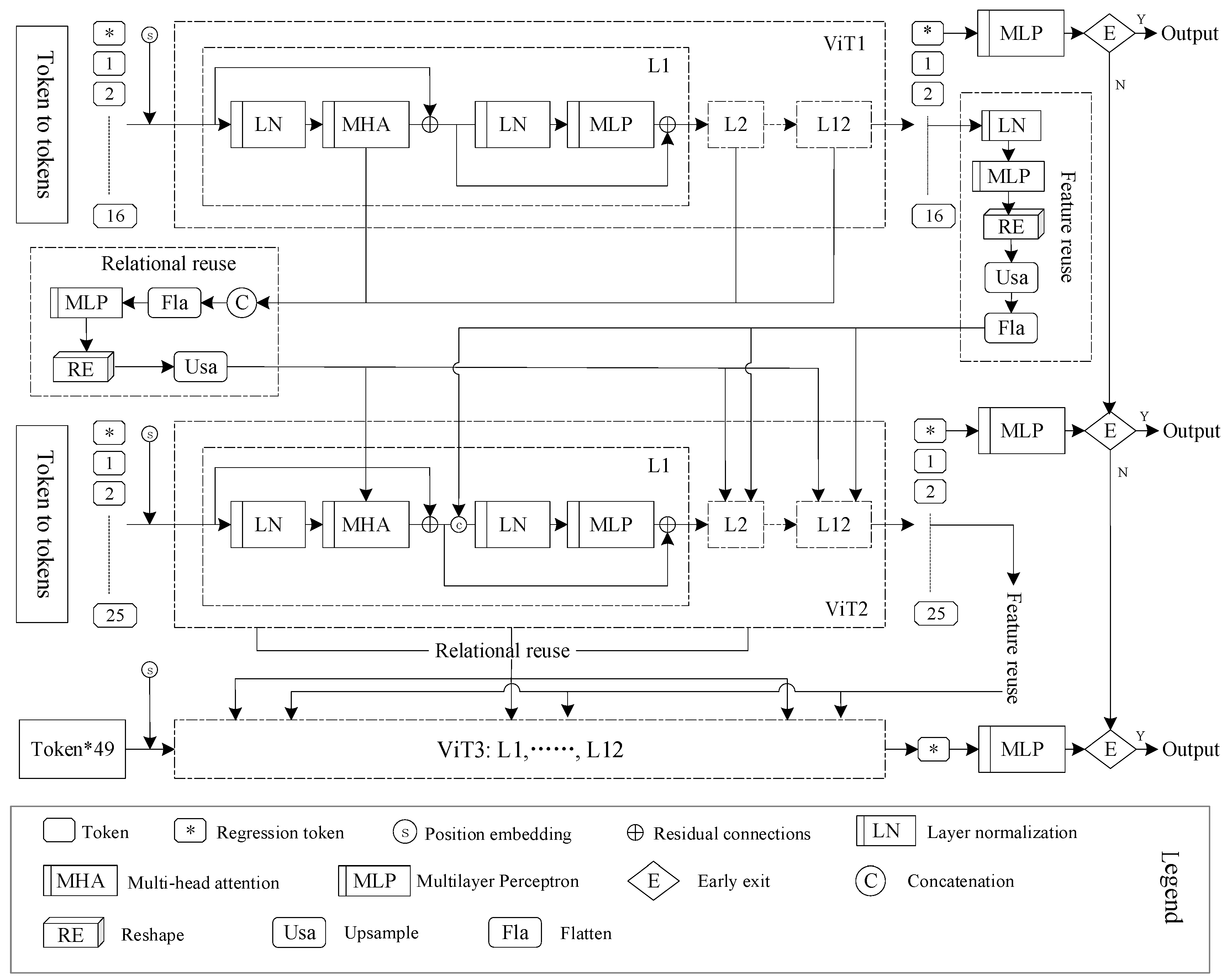
4. Model Construction

This research presents a dynamic neural network model constructed from a cascade of three sub-models for the purpose of batch assessment in real estate, aimed at enhancing the accuracy of the model, while improving inference efficiency using an early-exit mechanism. Unlike the primary benefits of adaptive depth found in MSDNet [39] and RANet [40], the dynamic neural network model designed in this study features complete model structures in each layer. The benefits are derived from the adaptive token counts, the relationship reuse mechanisms, and the feature reuse mechanisms. Detailed information is illustrated in Figure 1 below.

In conjunction with the research subject and data structure of this study, the fundamental structure of the dynamic neural network model was determined after multiple debugging sessions. The supplementary explanation of the model is as follows. First, due to the defects such as loss of information in the flattened data, this study utilizes the Tokens-to-token module to perform data encoding operations for the dynamic neural network model. Based on the dataset constructed for this study, the original sample data, once converted into tensors, have channel, height, and width dimensions of 1, 1, and 49, respectively. Through the Tokens-to-token module, the data are encoded into input tokens numbered at 16, 25, and 49 for three sub-model layers, each with an embedding dimension of 256. To prevent information loss during soft splitting, the data are segmented into overlapping soft-split blocks, thereby establishing a prior understanding that each soft-split block is related to its adjacent blocks. Each token within a soft-split block is then concatenated into a new token. Such operations allow for the aggregation of local structural information from the surrounding tokens and soft-split blocks and reduce the number of tokens. Second, the specific implementation process of the Tokens-to-token module involves converting the original sample data into tokens through soft splitting, and then encoding these into a specified number of token embeddings through iterative Tokens-to-token transformation, and the number of iterations set in this study is two. The iterative process is divided into reconstruction and soft splitting steps, with the tokens obtained from soft splitting provided to the next iteration.

In addition, based on the Deep–Narrow principle, this research designs the main trunk of the dynamic neural network model as a stacked 12-layer ViT model. The inference process for each layer of the sub-models can be represented as follows.

$$\left\{\begin{array}{c}{z_l}^{\prime }=MSA\left(LN\left(z_{l-1}\right)\right)+z_{l-1}\\ z_l=MLP\left(LN\left(z_l^{\prime }\right)\right)+{z_l}^{\prime }\end{array}\right.$$

(3)

In this formula, $z_{l-1}\in R^{N\times D}$ represents the input to each ViT layer, ${z_l}^{\prime }\in R^{N\times D}$ denotes the intermediate variables for each ViT layer, and $z_l\in R^{N\times D}$ signifies the output from each ViT layer. LN$\left(·\right)$ indicates layer normalization operations, MHA$\left(·\right)$ denotes multi-head attention operations, and MLP$\left(·\right)$ represents the multi-layer perceptrons. N is the number of input tokens, D refers to the dimensionality of token embeddings, $l\in \left\{\mathrm{1,2},3,\dots ,l\right\}$ and $l$ indicates the number of stacked ViT layers.

Moreover, this study introduces efficient mechanisms for feature reuse and relationship reuse to enhance information utilization. The final output $z_l^{up}$ from the upstream sub-model undergoes layer normalization and is processed by a multi-layer perceptron for nonlinearity, followed by reshaping and up-sampling to increase the spatial dimensions of the data. It is then flattened to align with the shape of the intermediate variables in the ViT layers of the downstream sub-model. Subsequently, the embedded features from each ViT layer of the downstream sub-model are incorporated into its intermediate variables to provide prior knowledge. In this process, the dimensionality of $E_l$ is set to a small value to ensure computational efficiency. In this model, it is set to 48. The designed relationship reuse mechanism specifically involves concatenating the attention matrices $A_l^{up}$ from each ViT layer of the upstream sub-model, followed by flattening, processing through a multi-layer perceptron for nonlinearity, reshaping, and up-sampling to produce the reused relational data. Finally, this relational data are segmented and individually incorporated into the attention matrices $A_l$ of each ViT layer in the downstream sub-model.

In the last, the problem addressed in this study is categorized as a regression problem. Consequently, the output is connected to a final output through a fully connected layer, representing the ultimate output of each sub-model layer in the dynamic neural network model. After each sub-model layer, a decision unit is placed, which can be implemented through various methods such as dropout, the additional training of a strategy network, and others. The study chooses to implement dropout to enable early stopping of the model, setting the dropout probabilities after each sub-model layer at 0.34, 0.5, and 1, respectively.

5. Mass Appraisal Results

5.1. Evaluation Dataset Split and Performance Metrics

Initially, the original dataset is divided into “K” equal-sized subsets, referred to as “folds”. Subsequently, one fold is selected as the validation set, while the remaining “K-1” folds serve as the training set. The model is then trained using the training set and evaluated on the validation set. This process is repeated “K” times, each time selecting a different validation set, and the average of the “K” evaluation results is used as the metric for assessing the model’s performance. To ensure robustness and generalization capability of the real estate batch evaluation model, there is also an interest in comparing the performance of the dynamic neural network model with that of multiple regression and Back Propagation (BP) neural network models. In this study, 10% of the data from the real estate batch evaluation dataset is randomly retained as a test set, with the remaining 90% is used for building the real estate mass appraisal model during the five-fold cross-validation stage, facilitating the division of the training and validation sets. The preprocessed dataset contains a total of 284,796 samples, each with 49 features. The training set comprises 72% of the dataset, the validation set contains 18%, and the test set contains 10%, with respective sample counts of 205,053, 51,263, and 28,480.

The dynamic neural network model constructed in this study for real estate batch evaluation is assessed using metrics such as R², MAPE, MAE, and RMSE. R² measures the goodness of fit of the regression model, with values closer to one indicating a higher ability of the model to explain the variability in the dependent variable. MAPE measures the relative accuracy of model predictions compared to actual observations, with values closer to 0 indicating higher predictive accuracy. MAE measures the average deviation of model predictions from actual observations, with values closer to 0 indicating smaller prediction errors. RMSE measures the average difference between model predictions and actual observations, with smaller values indicating smaller prediction errors and better predictive performance. The formulas for these metrics are as follows.

$$R^2=1-{\displaystyle \frac{{\sum }_{i=1}^n\left(y_i-{\widehat{y}}_i\right)}{{\sum }_{i=1}^n{(y_i-\overline{y})}^2}},\in \left[0,1\right]$$

(4)

$$\mathrm{MAPE}={\displaystyle \frac{1}{n}}{\sum }_{i=1}^n\left|{\displaystyle \frac{{\widehat{y}}_i-y_i}{y_i}}\right|\times 100,\in \left[0,+\infty \right]$$

(5)

$$\mathrm{MAE}={\displaystyle \frac{1}{n}}{\sum }_{i=1}^n\left|{\widehat{y}}_i-y_i\right|,\in \left[0,+\infty \right]$$

(6)

$$\mathrm{RMSE}=\sqrt{{\displaystyle \frac{1}{n}}{\sum }_{i=1}^n{\left({\widehat{y}}_i-y_i\right)}^2},\in \left[0,+\infty \right]$$

(7)

wherein, “n” represents the number of samples; $y_i$ denotes the actual observed values; ${\widehat{y}}_i$ refers to the predicted values; and $\overline{y}$ is the mean of the actual observed values.

5.2. Dynamic Neural Network Model Parameter Settings

This study employs the Pytorch v.2.0.0 framework to construct a dynamic neural network model for mass appraisal in real estate. The training of the model is carried out using an NVIDIA GeForce RTX 4090 (Zhongke Vision Technology Co., Ltd., Nanjing, China). Moreover, the optimal combination of parameters for training the dynamic neural network model is identified through a grid search method. Specific details are presented in

Table 6. Training settings of dynamic neural network.

Parameters	Parameter Setting
Size	512
Optimizer	Adamax, 0.0005
Loss function	Absolute loss function
Normalization	Normalize both the feature variable using Z-score standardization
Maximum number of iterations	75, 25

below.

5.3. Analysis of the Predictive Performance

Following the training settings of the dynamic neural network model, the model was trained, and the loss curves for both the training and validation sets are illustrated in Figure 2.

After the completion of training the dynamic neural network model, the prediction performance of the model was tested on both the training set and the validation set. The prediction results are shown in

Table 7. Predictive effect of dynamic neural network.

			MAPE	MAE	RMSE	R2
Fold1	Training set	Out1	6.582502	24.983809	70.879814	0.963392
		Out2	5.423621	20.559443	67.747513	0.966556
		Out3	5.238632	20.309767	67.341919	0.966955
	Validation set	Out1	8.287363	36.023987	83.487915	0.945973
		Out2	7.855760	34.425793	82.405426	0.947365
		Out3	7.688116	34.158836	83.090019	0.946487
Fold2	Training set	Out1	6.572026	24.770119	66.029747	0.967751
		Out2	5.854780	23.076227	65.405807	0.968357
		Out3	5.439150	21.075333	62.937225	0.970701
	Validation set	Out1	8.409850	35.866158	110.660057	0.910733
		Out2	7.951491	34.931698	110.155144	0.911545
		Out3	7.858031	34.483894	109.478119	0.912629
Fold3	Training set	Out1	7.153530	27.895760	74.618797	0.959092
		Out2	4.877150	18.729902	68.677696	0.965347
		Out3	4.623269	17.947077	66.300896	0.967704
	Validation set	Out1	8.751267	37.590763	93.737366	0.934191
		Out2	7.933979	34.954685	91.732445	0.936976
		Out3	7.611889	34.107365	90.031654	0.939291
Fold4	Training set	Out1	7.310944	29.143776	71.890549	0.960641
		Out2	4.759374	19.062849	62.082413	0.970648
		Out3	4.801227	19.073774	60.440533	0.972180
	Validation set	Out1	8.662125	39.258278	112.789848	0.916685
		Out2	7.944169	36.775803	111.652557	0.918357
		Out3	7.893782	36.247406	108.981903	0.922216
Fold5	Training set	Out1	6.830754	26.634205	72.839317	0.961583
		Out2	6.590454	26.017817	71.017235	0.963481
		Out3	5.525959	21.393906	68.016922	0.966502
	Validation set	Out1	8.618005	36.875156	88.689461	0.937333
		Out2	8.400989	36.270206	87.598625	0.938865
		Out3	7.958053	34.505462	86.413239	0.940508

.

The observations from the test results indicate that even the sub-models located in the shallow layers possess satisfactory predictive capabilities, and the predictive accuracy of each sub-model layer progressively improves in line with the theoretical expectations. This demonstrates the feasibility of employing the dynamic neural network model for mass appraisal in real estate.

5.4. Verification of the Effectiveness of Relationship and Feature Reuse

Theoretically, in the dynamic neural network model designed in this study, the enhancement in predictive performance of each sub-model layer is partly attributed to the mechanisms of relationship reuse and feature reuse. To validate the impact of these information reuse mechanisms on the predictive performance of sub-models within the dynamic neural network model, the model was retrained without implementing relationship and feature reuse under fixed training settings. After completing the training, tests were conducted again on both the training and validation sets, and the predictive results are shown in

Table 8. Predictive effect when relational reuse and feature reuse are not implemented.

			MAPE	MAE	RMSE	R2
Fold1	Training set	Out1	6.280432	24.876728	70.327866	0.963960
		Out2	5.083012	19.192019	68.024574	0.966282
		Out3	5.354226	21.244509	71.564575	0.962681
	Validation set	Out1	8.189092	36.558029	88.162560	0.939754
		Out2	7.846367	35.320896	90.475708	0.936551
		Out3	7.960067	36.351112	96.090004	0.928432
Fold2	Training set	Out1	5.279011	19.738766	53.211971	0.979056
		Out2	5.029600	18.977011	54.899643	0.977706
		Out3	4.318735	15.962884	58.919735	0.974322
	Validation set	Out1	8.084276	35.674702	110.581459	0.910859
		Out2	7.874303	35.196781	112.541832	0.907671
		Out3	7.774843	35.124073	119.312988	0.896227
Fold3	Training set	Out1	6.450404	25.219858	68.763458	0.965260
		Out2	6.172630	24.344225	73.040146	0.960805
		Out3	5.171786	19.415365	70.090607	0.963906
	Validation set	Out1	8.178583	35.226971	85.669205	0.945032
		Out2	8.333623	36.847321	96.665001	0.930016
		Out3	7.873034	35.293766	102.016411	0.922052
Fold4	Training set	Out1	6.542130	25.513079	65.900955	0.966926
		Out2	5.214116	19.814548	64.580650	0.968238
		Out3	4.968793	19.260939	65.202042	0.967624
	Validation set	Out1	8.226849	37.212627	112.413467	0.917240
		Out2	7.973021	36.835815	117.798599	0.909121
		Out3	8.087622	37.724483	122.078674	0.902397
Fold5	Training set	Out1	6.671336	26.329666	76.261787	0.957888
		Out2	5.925183	23.713930	74.932312	0.959344
		Out3	5.715444	22.097775	75.527740	0.958695
	Validation set	Out1	8.394048	36.008690	90.072845	0.935363
		Out2	8.168652	35.909081	93.465927	0.930401
		Out3	8.293054	36.042675	96.629173	0.925610

.

The observations from the dynamic neural network model’s performance without the implementation of relationship and feature reuse indicate that the fine granularity of original sample data does not necessarily have a positive effect on the assessment results of each sub-model layer due to the occurrence of overfitting. Comparing the predictive performance of sub-model layers in the dynamic neural network model before and after applying these two information reuse mechanisms, it is evident that they alleviate the issue of overfitting in the deep sub-models. Additionally, they enhance the predictive accuracy of each sub-model layer with a minimal increase in computational load, aligning with the theoretical expectations. Therefore, relationship and feature reuse hold practical value in the dynamic neural network model designed in this study.

5.5. Real Mass Appraisal Evaluation Results

To achieve adaptive inference during the testing phase, a decision unit is placed after each sub-model layer within the dynamic neural network model. This unit is designed to adaptively determine whether to activate the downstream sub-models or execute exits based on different input samples, thereby enhancing the model’s inference efficiency and interpretability. Subsequently, the model’s appraisal performance is tested on both the training and validation sets, with the results of the “5-fold” cross-validation presented in

Table 9. Evaluation results of dynamic neural network.

		MAPE	MAE	RMSE	R2
Fold1	Training set	5.733302	21.887262	68.645737	0.965663
	Validation set	7.944661	34.873470	83.153336	0.946405
Fold2	Training set	5.937993	22.919348	65.170738	0.968584
	Validation set	8.090828	35.148426	110.563599	0.910888
Fold3	Training set	5.539233	21.470678	70.377716	0.963610
	Validation set	8.148492	35.579693	91.269135	0.937611
Fold4	Training set	5.601123	22.318249	64.984169	0.967840
	Validation set	8.208256	37.563663	111.897202	0.917999
Fold5	Training set	6.265540	24.529627	71.089607	0.963407
	Validation set	8.364384	36.068787	88.551712	0.937527
Average	Training set	5.815438	22.625033	68.053593	0.965821
	Validation set	8.151324	35.846808	97.086996	0.930086

.

From the results of cross-validation, it is evident that the dynamic neural network model demonstrates an average MAPE, MAE, RMSE, and R² of 5.815438, 22.625033, 68.053593, and 0.965821, respectively, on the training set, and 8.151324, 35.846808, 97.086996, and 0.930086, respectively, on the validation set. The overall appraisal results are favorable, exhibiting not only high precision during regression fitting, but also maintaining good generalization capabilities during external evaluation. Further observations of the model‘s performance across different folds show that the evaluation metrics for the training and validation sets are mostly similar, indicating the good generalization ability and stability of the model. Only in the “second and fourth folds”, the performance in terms of RMSE and R² on the validation set appears slightly inadequate. This phenomenon may be attributed to the limitations in data quantity and variations in the distribution of datasets across folds. The dynamic neural network model is capable of fulfilling tasks related to real estate mass appraisal.

6. Model Comparative Analysis

With the current real estate mass appraisal practices, the commonly used forms of multiple regression models include linear, logarithmic, log-linear, and linear-log forms. Upon comparing the OLS fitting results, it was found that the logarithmic form of the multiple regression model performed optimally. Consequently, this study elects to compare the dynamic neural network model with the logarithmic form of the multiple regression model and the commonly used BP neural network model. The construction and analysis of the multivariate regression model were based on the analytical process described in ref. [41].

The final form of the multiple regression model can be validated through various econometric tests. The parameter settings for the BP neural network model are guided not only by the experience from existing results, but primarily by the settings that optimize model performance. The samples used for “5-fold” cross-validation serve as a new training set. According to the training settings described earlier, the dynamic neural network model, multiple regression model, and BP neural network model are retrained, and then tested on the training and test sets. The test results, as shown in

Table 10. Comparison of evaluation effects of real estate mass appraisal models.

		MAPE	MAE	RMSE	R2
Dynamic neural network model	Training set	5.036730	19.160849	62.783176	0.970929
	Validation set	7.444632	33.046982	96.708458	0.930406
Multivariate regression model	Training set	14.571461	63.687946	137.256558	0.861058
	Validation set	14.545142	63.470088	139.588094	0.855009
BP neural network model	Training set	16.705354	65.148232	117.553528	0.898085
	Validation set	16.640142	65.064880	116.835655	0.898423

, indicate that the appraisal metrics for the dynamic neural network model, multiple regression model, and BP neural network model are closely matched on both the training and test sets, suggesting that all the models are in a good state of fit.

Comparative analysis between the multiple regression model and the BP neural network model on the test set reveals that the BP neural network model performs better in terms of RMSE and R², but slightly worse in MAPE and MAE. This indicates that compared to the multiple regression model, the BP neural network model shows a superior performance in capturing the overall error magnitude and variability of the target variable, but is slightly inferior in terms of average error magnitude and relative error. Compared to the multiple regression model and the BP neural network model, the dynamic neural network model shows an improvement in MAPE by 7.10051 and 9.19551, in MAE by 30.423106 and 32.017898, in RMSE by 42.879636 and 20.127197, and in R² by 0.075397 and 0.031983, respectively, on the test set. These significant improvements in the key performance indicators demonstrate its superior predictive accuracy, ability to handle large errors, and enhanced capability in explaining the variability of the target variable compared to the multiple regression and BP neural network models. The dynamic neural network model designed in this study effectively addresses complex nonlinear problems and can be employed for real estate mass appraisal to achieve optimal results.

7. Conclusions

This study has designed a dynamic neural network model for real estate mass appraisal, which consists of a cascade of three sub-models, each with a complete structural configuration. The benefit gains stem from the adaptive token quantity, and the relationship reuse mechanism, and the feature reuse mechanism. The number of input tokens for each sub-model layer increases progressively, while the encoding dimension of each token remains constant, thereby achieving a more granular data representation layer by layer. The main trunk of the model consists of sub-model layers stacked with an equal number of ViT layers, which serve as feature extraction units to extract deep information from the input tokens. Additionally, in this section, relationship and feature reuse mechanisms are employed to recycle valuable information extracted by the upstream sub-models, enhancing the efficiency of information utilization. In the model’s output section, a fully connected layer is implemented to transform the regression tokens refined by each sub-model into the final evaluation results. Moreover, a decision unit is placed after each sub-model layer, responsible for adaptively determining the activation of downstream sub-models during the inference stage based on different test samples until a convincing prediction result is obtained.

Data from January 2015 to June 2023 on second-hand housing transactions in Shanghai were collected, totaling 327,286 sample cases. After data processing, 284,796 cases were included in the empirical analysis, with 49 real estate characteristic indicators used to validate the performance of the new model. The results from cross-validation indicate that the dynamic neural network model generally performs well, demonstrating high precision during regression fitting and maintaining good generalizability during external evaluations. The observations of the model’s performance across different “folds” show that the appraisal metrics for both the training and validation sets are closely matched, indicating the good stability of the model. Compared to the multiple regression model and the BP neural network model, the dynamic neural network model shows significant improvements in prediction accuracy, error handling, and explaining the variability of the target variable. The dynamic neural network model designed in this study effectively addresses complex nonlinear problems and can be used for real estate mass appraisal to achieve optimal results.

However, in exploring machine learning-based methods for real estate mass appraisal, there are still numerous limitations and technical issues that need to be addressed. For example, how to intelligently assess the complexity of samples to create dynamic neural network structures and whether it is possible to consider the cyclical capitalization approach [42], thereby integrating real estate market cyclical factors with the model. In summary, there is still significant room for optimization in sample-adaptive deep neural network models, and the prospects for the application of dynamic neural network models in real estate mass appraisal are very broad.

References

1. Yousfi, S.; Dubé, J.; Legros, D.; Thanos, S. Mass appraisal without statistical estimation: A simplified comparable sales approach based on a spatiotemporal matrix. Ann. Reg. Sci. 2020, 64, 349–365. [Google Scholar] [CrossRef]
2. Wang, D.; Li, V.J. Mass appraisal models of real estate in the 21st Century: A systematic literature review. Sustainability 2019, 11, 7006. [Google Scholar] [CrossRef]
3. Dimopoulos, T.; Bakas, N.P. Sensitivity analysis of machine learning models for the mass appraisal of real estate. Case study of residential units in Nicosia, Cyprus. Remote Sens. 2019, 11, 3047. [Google Scholar] [CrossRef]
4. Arribas, I.; García, F.; Guijarro, F.; Oliver, J.; Tamošiūnienė, R. Mass appraisal of residential real estate using multilevel modelling. Int. J. Strateg. Prop. Manag. 2016, 20, 77–87. [Google Scholar] [CrossRef]
5. McCluskey, W.; McCord, M.; Davis, P.; Haran, M.; McIlhatton, D. Prediction accuracy in mass appraisal: A comparison of modern approaches. J. Prop. Res. 2013, 30, 239–265. [Google Scholar] [CrossRef]
6. Zhang, R.; Du, Q.; Geng, J.; Liu, B.; Huang, Y. An improved spatial error model for the mass appraisal of commercial real estate based on spatial analysis: Shenzhen as a case study. Habitat Int. 2015, 46, 196–205. [Google Scholar] [CrossRef]
7. Uberti, M.S.; Antunes, M.A.H.; Debiasi, P.; Tassinari, W. Mass appraisal of farmland using classical econometrics and spatial modeling. Land Use Policy 2018, 72, 161–170. [Google Scholar] [CrossRef]
8. Bencure, J.C.; Tripathi, N.K.; Miyazaki, H.; Ninsawat, S.; Kim, S.M. Development of an innovative land valuation model (iLVM) for mass appraisal application in sub-urban areas Using AHP: An Integration of theoretical and practical approaches. Sustainability 2019, 11, 3731. [Google Scholar] [CrossRef]
9. Zhao, Y.; Shen, X.; Ma, J.; Yu, M. Path selection of spatial econometric model for mass appraisal of real estate: Evidence from yinchuan. Int. J. Strateg. Prop. Manag. 2023, 27, 304–316. [Google Scholar] [CrossRef]
10. Kilpatrick, J. Expert systems and mass appraisal. J. Prop. Invest. Financ. 2011, 29, 529–550. [Google Scholar] [CrossRef]
11. Doszyń, M. Might expert knowledge improve econometric real estate mass appraisal? J. Real Estate Financ. Econ. 2022, 1–22. [Google Scholar] [CrossRef]
12. Zurada, J.; Levitan, A.S.; Guan, J. A Comparison of regression and artificial Intelligence methods in a mass appraisal context. J. Real Estate Res. 2011, 33, 349–387. [Google Scholar] [CrossRef]
13. Hong, J.; Choi, H.; Kim, W.S. A house price valuation based on the random forest approach: The mass appraisal of residential property in South Korea. Int. J. Strateg. Prop. Manag. 2020, 24, 140–152. [Google Scholar] [CrossRef]
14. Morano, P.; Tajani, F.; Locurcio, M. Multicriteria analysis and genetic algorithms for mass appraisals in the Italian property market. Int. J. Hous. Mark. Anal. 2018, 11, 229–262. [Google Scholar] [CrossRef]
15. Morano, P.; Rosato, P.; Tajani, F.; Manganelli, B.; Di Liddo, F. Contextualized property market models vs. Generalized mass appraisals: An innovative approach. Sustainability 2019, 11, 4896. [Google Scholar] [CrossRef]
16. Reyes-Bueno, F.; García-Samaniego, J.M.; Sánchez-Rodríguez, A. Large-scale simultaneous market segment definition and mass appraisal using decision tree learning for fiscal purposes. Land Use Policy 2018, 79, 116–122. [Google Scholar] [CrossRef]
17. Antipov, E.A.; Pokryshevskaya, E.B. Mass appraisal of residential apartments: An application of random forest for valuation and a CART-based approach for model diagnostics. Expert Syst. Appl. 2012, 39, 1772–1778. [Google Scholar] [CrossRef]
18. Yilmazer, S.; Kocaman, S. A mass appraisal assessment study using machine learning based on multiple regression and random forest. Land Use Policy 2020, 99, 104889. [Google Scholar] [CrossRef]
19. Chun Lin, C.; Mohan, S.B. Effectiveness comparison of the residential property mass appraisal methodologies in the USA. Int. J. Hous. Mark. Anal. 2011, 4, 224–243. [Google Scholar] [CrossRef]
20. McCluskey, W.; Davis, P.; Haran, M.; McCord, M.; McIlhatton, D. The potential of artificial neural networks in mass appraisal: The case revisited. J. Financ. Manag. Prop. Constr. 2012, 17, 274–292. [Google Scholar] [CrossRef]
21. Yacim, J.A.; Boshoff, D.G.B.; Khan, A. Hybridizing Cuckoo Search with Levenberg-Marquardt algorithms in optimization and training of ANNs for mass appraisal of properties. J. Real Estate Lit. 2016, 24, 473–492. [Google Scholar] [CrossRef]
22. Yacim, J.A.; Boshoff, D.G.B. Combining BP with PSO algorithms in weights optimisation and ANNs training for mass appraisal of properties. Int. J. Hous. Mark. Anal. 2018, 11, 290–314. [Google Scholar] [CrossRef]
23. Torres-Pruñonosa, J.; García-Estévez, P.; Prado-Román, C. Artificial neural network, quantile and Semi-Log regression modelling of mass appraisal in Housing. Mathematics 2021, 9, 783. [Google Scholar] [CrossRef]
24. Iban, M.C. An explainable model for the mass appraisal of residences: The application of tree-based machine learning algorithms and interpretation of value determinants. Habitat Int. 2022, 128, 102660. [Google Scholar] [CrossRef]
25. Carranza, J.P.; Piumetto, M.A.; Lucca, C.M.; Da Silva, E. Mass appraisal as affordable public policy: Open data and machine learning for mapping urban land values. Land Use Policy 2022, 119, 106211. [Google Scholar] [CrossRef]
26. McCord, M.; Lo, D.; Davis, P.; McCord, J.; Hermans, L.; Bidanset, P. Applying the geostatistical eigenvector spatial filter approach into regularized regression for Improving prediction accuracy for mass appraisal. Appl. Sci. 2022, 12, 10660. [Google Scholar] [CrossRef]
27. Bilgilioglu, S.S.; Yilmaz, H.M. Comparison of different machine learning models for mass appraisal of real estate. Surv. Rev. 2023, 55, 32–43. [Google Scholar] [CrossRef]
28. Dearmon, J.; Smith, T.E. A Local gaussian process regression approach to mass appraisal of residential properties. J. Real Estate Financ. Econ. 2024, 1–19. [Google Scholar] [CrossRef]
29. Yasnitsky, L.N.; Yasnitsky, V.L.; Alekseev, A.O. The complex neural network model for mass appraisal and scenario forecasting of the urban real estate market value that adapts Itself to space and time. Complexity 2021, 2021, 5392170. [Google Scholar] [CrossRef]
30. Han, Y.; Huang, G.; Song, S.; Yang, L.; Wang, H.; Wang, Y. Dynamic neural networks: A survey. IEEE Trans. Pattern Anal. Mach. Intell. 2021, 44, 7436–7456. [Google Scholar] [CrossRef]
31. Chau, K.W.; Chin, T.L. A critical review of literature on the hedonic price model. Int. J. Hous. Sci. Its Appl. 2003, 27, 145–165. [Google Scholar]
32. Walacik, M.; Chmielewska, A. Real Estate Industry Sustainable Solution (Environmental, Social, and Governance) Significance Assessment-AI-Powered Algorithm Implementation. Sustainability 2024, 16, 1079. [Google Scholar] [CrossRef]
33. Zhan, W.; Hu, Y.; Zeng, W.; Fang, X.; Kang, X.; Li, D. Total Least Squares Estimation in Hedonic House Price Models. ISPRS Int. J. Geo-Inf. 2024, 13, 159. [Google Scholar] [CrossRef]
34. Rey-Blanco, D.; Zofío, J.L.; González-Arias, J. Improving hedonic housing price models by integrating optimal accessibility indices into regression and random forest analyses. Expert Syst. Appl. 2024, 235, 121059. [Google Scholar] [CrossRef]
35. Cardone, B.; Di Martino, F.; Senatore, S. Real estate price estimation through a fuzzy partition-driven genetic algorithm. Inf. Sci. 2024, 667, 120442. [Google Scholar] [CrossRef]
36. Unel, F.B.; Yalpir, S. Sustainable tax system design for use of mass real estate appraisal in land management. Land Use Policy 2023, 131, 106734. [Google Scholar] [CrossRef]
37. Tian, Y.; Yang, J.P. Application of geographic Information system on urban residential real estate mass appraisal. Appl. Mech. Mater. 2015, 744, 1665–1668. [Google Scholar] [CrossRef]
38. Chen, S.Q.; Wang, H.W. Machine Learning-Based Mass Appraisal Model for Real Estate, Statistics and Decision Making; Tongfang CNKI (Beijing) Technology Co., Ltd.: Beijing, China, 2020; Volume 36, pp. 181–185. [Google Scholar] [CrossRef]
39. Huang, G.; Chen, D.; Li, T.; Wu, F.; Van Der Maaten, L.; Weinberger, K.Q. Multi-scale dense networks for resource efficient image classification [EB/OL]. arXiv 2017. https://arxiv.org/abs/1703.09844.
40. Yang, L.; Han, Y.; Chen, X.; Song, S.; Dai, J.; Huang, G. Resolution adaptive networks for efficient inference. In Proceedings of the IEEE/CVF Conference on Computer Vision and Pattern Recognition, Seattle, WA, USA, 14–19 June 2020; pp. 2366–2375. [Google Scholar]
41. De Salvo, M.; Signorello, G.; Cucuzza, G.; Begalli, D.; Agnoli, L. Estimating preferences for controlling beach erosion in Sicily. Aestimum 2018, 72, 27–38. [Google Scholar]
42. d’Amato, M.; Cucuzza, G. Cyclical capitalization: Basic models. Aestimum 2022, 80, 45–54. [Google Scholar] [CrossRef]
Figure 1. The dynamic neural network model for real estate mass appraisal.
Buildings 14 02199 g001
Figure 2. Loss curves. (a) Loss curves of fold 1; (b) loss curves of fold 2; (c) loss curves of fold 3; (d) loss curves of fold 4; (e) loss curves of fold 5.
Buildings 14 02199 g002