Abstract
The article discusses a solution to the relevant task of analyzing and designing modular buildings made of blocks to be used in industrial and civil engineering. A block that represents a container is a combination of plate and beam systems. The criteria for its failure include both the strength of the individual elements and the loss of stability in a corrugated web. Methods of engineering analysis are hardly applicable to this system. Numerical analysis based on the finite element method is time-consuming, and this fact limits the number of design options for modular buildings made of blocks. Adjustable machine learning models are proposed as a solution to these problems. Decision trees are made and clustered into a single ensemble depending on the values of the design parameters. Key parameters determining the structures of decision trees include design steel resistance values, types of loads and the number of loadings, and ranges of rolled sheet thickness values. An ensemble of such models is used to take into account the nonlinear strain of elements. Piecewise approximation of the dependencies between components of the stress–strain state is used for this purpose. Linear regression equations are subjected to feature binarization to improve the efficiency of nonlinearity projections. The identification of weight coefficients without laborious search optimization methods is a distinguishing characteristic of the proposed models of steel blocks for modular buildings. A modular building block is used to illustrate the effectiveness of the proposed models. Its purpose is to accommodate a gas compressor of a gas turbine power plant. These machine learning models can accurately spot the stress–strain state for different design parameters, in particular for different corrugated web thickness values. As a result, ensemble models predict the stress–strain state with the coefficient of determination equaling 0.88–0.92.
1. Introduction
Research undertakings focused on modular buildings and their constituent blocks have evolved in the following five principal directions:
- -
- Analysis of the stress–strain state, design, and optimization of modular building blocks as a whole (1);
- -
- Research and improvement of nodal connections in modules subjected to different types of loads (lateral, seismic, impact, etc.) (2);
- -
- Evaluation of the resistance of modular buildings and individual blocks to progressive collapse triggered by emergency loads and effects causing the inability of individual nodes or structural elements to resist loads (3);
- -
- New materials in modular construction (4);
- -
- Development and improvement of assembly technologies and introduction of new types of modular buildings (5).
Each direction encompasses several relevant research projects. Indeed, as for Direction (1), work [1] demonstrates that the use of modular buildings is particularly efficient in construction from the standpoint of the life cycle cost of a structure. However, issues of energy-saving design are in the spotlight in the process of building operation. These issues can be solved by using new materials to make block elements, contributing advanced structural solutions and technologies to nodal connections at the stages of installation and operation. The stages of transportation and recycling can hardly affect the life cycle costs. The author of work [2] focuses on high relevance of modular construction in the context of environmental challenges. In addition to the importance of the design of modular buildings, the authors address optimization issues. Towards this end, they propose a rigorous formulation of the Lagrange multiplier method to minimize the mass of steel blocks. In this case, a single block and a system of blocks can be optimized, and the frequencies of natural vibrations in a system of blocks can be restrained.
Several studies dealing with structural design for emergency situations, including pandemics [3], demonstrate the need to optimize design solutions in terms of the mass of load-bearing structures of modular blocks. In this work, the authors report the case of a 24% reduction in the consumption of materials compared to conventional designs. Another problem requiring the design of modular buildings is the shortage of housing due to population growth. Another step towards optimal solutions to this problem is made in [4]. SAP2000 and MATLAB r2020a software packages are jointly used there to solve the problems of computation and optimization. The authors assume that high modular buildings (up to 15 floors) built using sets of corner blocks are effective without any targeted actions taken to ensure the resistance of a facility to lateral loads, including wind loads. The methods proposed by the authors are also applicable to freestanding blocks. Work [5] summarizes the design experience related to the design and construction of facilities consisting of prefabricated 3D blocks.
Building information modeling (BIM) technologies are vital for research undertakings focused on the design of modular buildings. Work [6] describes the process of structural design focused on accelerated structural solutions based on values of characteristic dimensions. These solutions stem from connections made between design parameters in the BIM environment. Each parameter is attached to a range of acceptable values and analytical dependencies used to calculate the values of other dependent parameters. This method can also be applied to the modular block dismantling procedure. A generative design technology is developed in work [7]. It employs the BIM concept to describe a modular block using a new class of Industry Foundation Classes (IFC) devised for a particular type of facility. In this case, the topology of an oriented graph is employed to structure information about a facility.
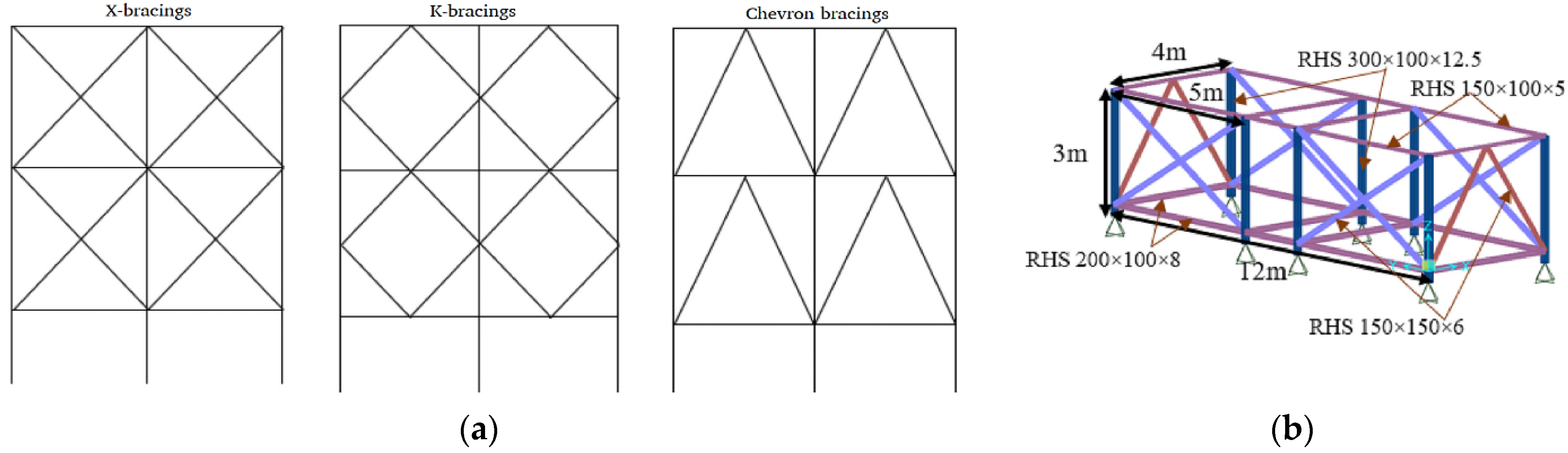
The design of modular multi-storey buildings is closely related to the study of their resistance to lateral loads, particularly wind loads. A study of the effectiveness of different types of bracings needed to ensure the stiffness of block systems is shown in Figure 1 [8].
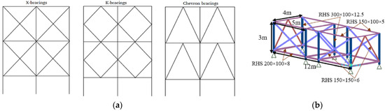
Figure 1.
Bracings in the frame structure designed for several blocks (a) and for an independent modular block (b).
In addition to such bracings, authors recommend using discrete diaphragms and increasing the stiffness of nodal connections. In article [9], numerical studies are carried out in LS-DYNA to evaluate the contribution of particular structural elements to the performance of a modular block frame. It is found that the most important parameters affecting structural safety are the stiffness of nodal connections between modules, the number of racks in a block, and the torsional stiffness of a facility. To further this research project, the authors of work [10] propose and numerically verify an equation describing the overall stability of a facility and determine design length ratios to evaluate the stability of individual elements. The recommendation is to design facilities whose height-to-width ratios do not exceed 3. Work [11] addresses the design of inter-module connections, including corner-tied connections and discontinuous modular diaphragms. Improved finite element models are proposed. In addition to static tests, dynamic tests of modular buildings are conducted. The most important parameter is the damping capacity of connections between blocks. These experimental studies are described in [12]. The dynamic loading history was recorded using a data capture system; vibration modes, damping coefficients, and natural vibration frequencies were identified.
Direction (2) focuses on the following principal issues: development of new types of connections; their numerical computation and experimental study; and simplified analytical dependencies required for design purposes. Let us analyze such works. The authors of work [13] designed a bolt-free vertical and horizontal inter-module connection (Figure 2a).
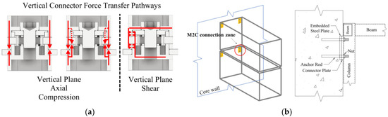
Figure 2.
Types of connections: inter-module connection (a), connection between a module and a wall of the stiffening core in a building (b).
The authors of work [14] developed and studied the connections between the stiffening core and the system of volumetric blocks (modules), as shown in Figure 2b. The figure shows that this connection is fully bolted. Numerical studies have shown that this connection fails under cyclic loading as a result of shear strain in anchor bolts. Therefore, design principles were developed for such connections to ensure that the required strength and ductility of individual elements were achieved. Article [15] focuses on a characteristic experiment in the field of research of inter-module connections. This article determines three possible levels of research: the first one is M, module research; the second one is F, frame research; and the third one is J, joint research. A classification of the joints between elements and their strengths and weaknesses are provided, and the efficiency of application of different types of nodes in frame structures is experimentally justified. Towards this end, article [16] offers a new design solution for corner connections between modules. A corner connection has a bolt made of a shape memory alloy and a high-damping rubber core. It reduces global damage to nodes during structural hysteresis of the system as a whole, as well as during the assembly and disassembly of individual building modules.
Another characteristic inter-module connection has a plug-in connector, such as the one proposed in work [17]. A cross-shaped plug-in connector connects modules. The author proves that the parameters of this connector affect the shear resistance and initial torsional stiffness of an inter-module connection. Due to the complexity of computations of this type, formulas of some parameters for this connection are provided in the form of regression equations. The fact is that some joints have weaknesses due to problematic disassembly, spaciousness requirements, and sensitivity to installation errors. These problems are largely solved by rotary connections [18] and shear bolted and splined connections [18,19]. In addition, there is a problem with the vulnerability of modular buildings to seismic effects. Hence, researchers focus on designing ductile nodes with pronounced plastic properties [20]. More information about inter-module connections and their mechanical performance are provided in the review article in [21].
Direction (3) is the most important and understudied field of modular buildings and their research. Most frequent emergency effects considered in practical studies include the failure of columns in 3D blocks of buildings or modules (for example, corner modules). An alternative load path method is used to study the resistance to progressive collapse [22,23]. In these works, an integrated problem investigating the parameters of element cross-sections, inter-module connections, and numbers of building storeys is solved depending on peak dynamic loads. In particular, the values of dynamic response factors, equaling 1.6–1.9, were determined in [23]. It is noteworthy that the removal of a corner column does not have a great effect on progressive collapse, as is the case for standard-design buildings. Work [24] shows that the strength factor (supplementary loading) of columns is 0.8 for modular buildings with cantilevers. Many works, in particular work [25], emphasize the absence of regulations governing emergency situations during the construction of modular buildings. In particular, inter-module connections, being the most sensitive parts of buildings, are in need of such regulations [26]. Also, several works have focused on the importance of research in fields other than mechanical damage. Thus, pulse impact design is also relevant [27], as is fire-induced damage and its development and effects on the strength of modular buildings [28]. Several works have focused on such emergencies as the failure of ground-floor corner or central modules under different scenarios [29,30]. These works identify collapse mechanisms and show that the key role belongs to (1) the tensile and shear stiffness of inter-module connections, as well as (2) the prevention of plastic hinges in the beam structures of blocks.
Some basic research undertakings focused on direction (4) have analyzed the efficiency of modules made of different materials throughout their life cycles. New materials are also used to connect blocks. Work [31] analyzes the strengths and weaknesses of steel and concrete blocks in construction. The authors analyze the overall efficiency of materials with positive effects on the environment. Some articles have analyzed blocks made of new and traditional materials. The authors of work [32] suggest using composite steel-reinforced concrete structures to make building frames, as well as using concrete slabs to make enclosing structures. These solutions allow buildings to resist lateral loads more effectively. Work [33] shows the effectiveness of monolithic reinforced concrete modules for low-rise and high-rise construction projects. The authors of work [34] assume that the installation and dismantling of modular blocks can be accelerated by grouted sleeves as weld-free and bolt-free connections between modules. In general, new materials, including composite materials, greatly increase the efficiency of modular construction, and more information about this can be found in the review article [35].
The most important field of modular construction research, focused on direction (5), is the development and improvement of module installation technologies. Principal trends are listed in [36]. They include high accuracy and reliability of installation works, installation simplicity, absence of stresses concentrated in connection nodes, prevention of accidental dismantling, etc. Installation can become faster and more accurate if remotely or automatically controlled robotic manipulators are used [37]. Certain installation problems are the poor quality of nodal connections or damaged nodal connections. To solve this problem, the authors of work [38] proposed special self-locking inter-module nodes. Self-locking steel connectors are developed on the basis of the same principle [39]. Lock elements have plastic properties (their plasticity coefficient equals 4). In summary, it is noteworthy that the study, analysis, and design of modular construction facilities, including single containers used for transportation and housing purposes, is a particularly relevant task that affects both the economy [40] and the environment [40].
The growing demand for design and construction of modular structures requires methods of fast evaluation and prediction of parameters of structural solutions. Intensively developing artificial intelligence technologies can tackle this challenge. The k-nearest neighbors (KNN) algorithm can predict the parameters of steel structures [41,42], and the same is true for various types of machine learning models, including support vectors; gradient boosting; regression equations [43,44]; and ensemble methods such as decision trees, random forest [45,46], etc.
This paper proposes a research approach intended to realize the design of a corrugated web modular block along direction (1) using machine learning. Towards this end, limit state criteria are set to determine structural safety in the case of a loss of web strength or stability, as described in Section 2.1. Section 2.2 describes a method of structural analysis that takes into account nonlinear strains. This method is used to design a computational finite element model. This model is used to generate machine learning data, which are provided in Section 2.3. Machine learning is based on the co-use of decision trees, each of which is attached to a combination of design parameters of a modular block. Values of equivalent von Mises strains are found to demonstrate the effectiveness of predictions made by the ensemble model and developed by the authors.
2. Methods and Materials
2.1. Problem Statement
2.1.1. A Geometric and Physical Model of a Modular Block Designed for a Gas Compressor at a Gas Turbine Power Plant
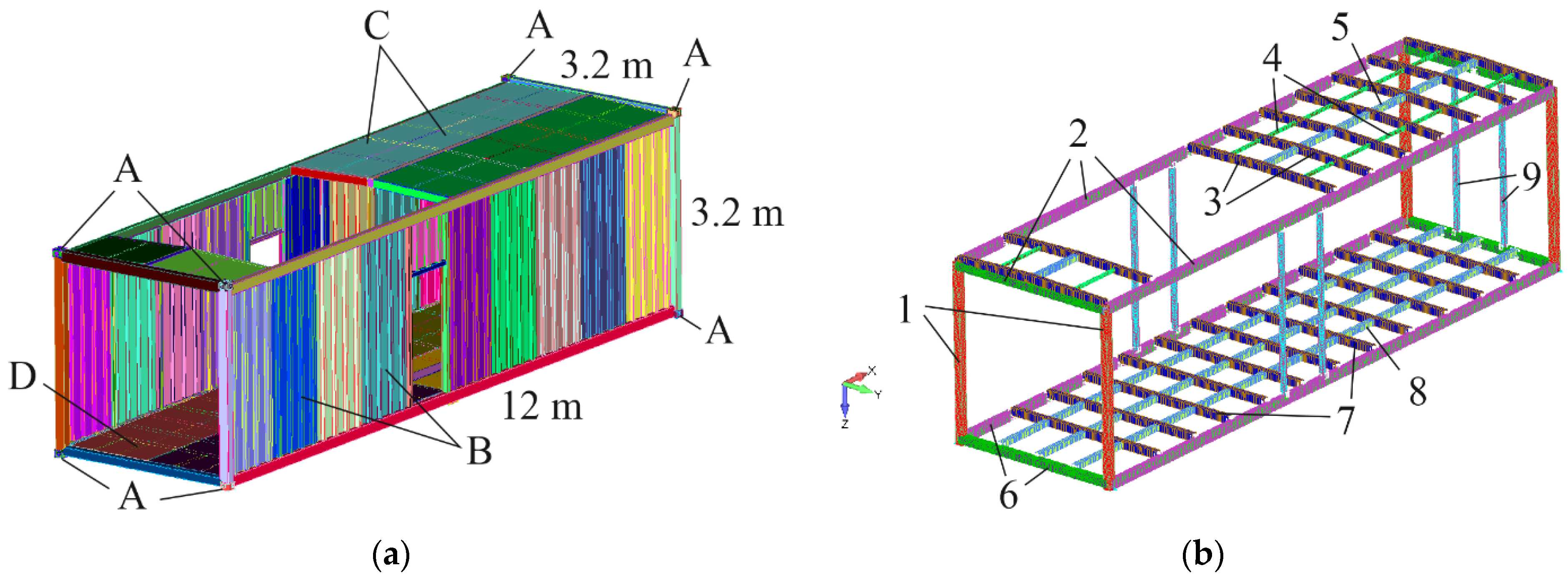
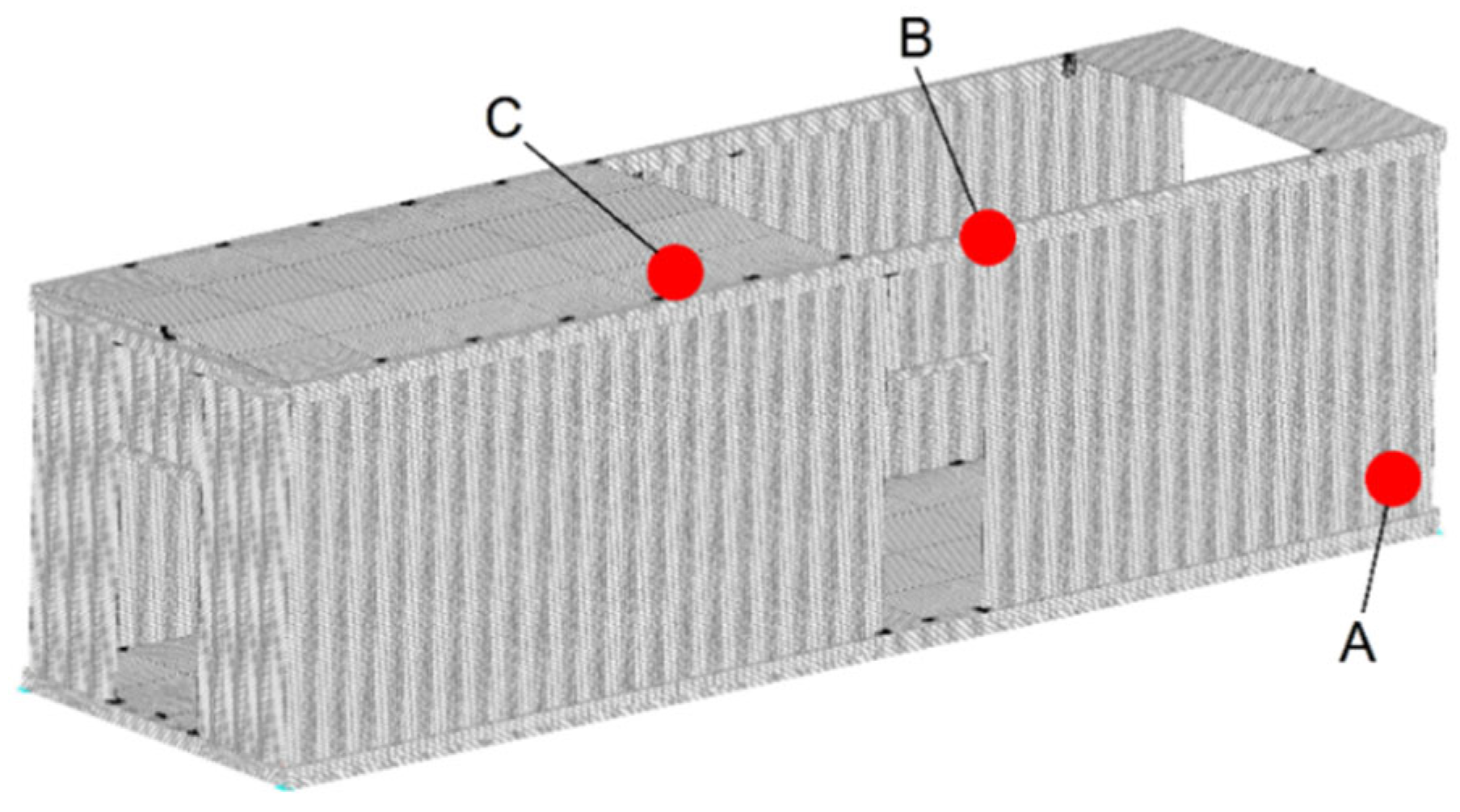
A modular building is a 3D system with overall dimensions equaling 12m × 3.2m × 3.2 m. The block transfers load to the neighboring blocks or the foundation at corner points A (see Figure 3). When the system is analyzed as a whole, its strains are similar to those in a beam structure. In this case, its top and bottom parts are in compression and tension, respectively. In the case under consideration, the structure’s span-to-height ratio is L/H = 3.75, which is less than L/H < 5. Therefore, whenever a corrugated web is analyzed, large shear strains should be taken into account (Bernoulli’s hypothesis is not satisfied).
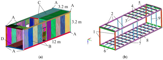
Figure 3.
A geometric model as the subject of research: (a) A are support fittings, B is a corrugated web, C is a flat deck sheet, and D is a floor sheet. The frame of the modular block (b): 1 represents corner racks, 2 represents top contour beams, 3 represents secondary beams, 4 represents roof support beams, 5 represents ridged bracing, 6 represents bottom contour beams, 7 represents secondary floor beams, 8 represents floor bracings, and 9 represents middle racks.
The structure has a frame with stiffly connected nodes. The frame has top and bottom contour beams and corner racks connecting the top and bottom contour beams. These elements are made of rectangular pipes. The floor and the top have bracings. The webs, floor, and top steel sheets are welded to the pipes. The sheets have thicknesses of 4 mm and are supported by angle bars. The thicknesses of the floor and top sheets remain unchanged for computation purposes. All elements of the block are made of structural steel with a standard yield strength of 245 MPa.
2.1.2. Criteria of Limit State for Elements
The limit states considered here are those that are most relevant for evaluating the ultimate load acting on a facility. These states include:
- -
- Serviceability loss of a structure (I);
- -
- Strength loss of structural elements (II);
- -
- Stability loss of a corrugated web (III).
Let us formulate the boundary equations expressing the strain criteria for the limit states, taking into account the practice in the analysis and design of modular structures. For state (I):
where are von Mises strains conveying the load acting on a structure; and are strains for cases of stresses equal to the yield strength of steel and the ultimate uniaxial tensile strength, respectively.
For state (II):
where , are the same strains as in Formula (1), and 0.85 is a coefficient that takes into account the initial geometric imperfections of the elements and their nodal connections, as well as defects caused by the poor quality of work performed in the process of the manufacturing of the structure.
Local and overall stability loss can be distinguished for state (III). The curve in Figure 4 should be analyzed in order for the criterion to be developed.
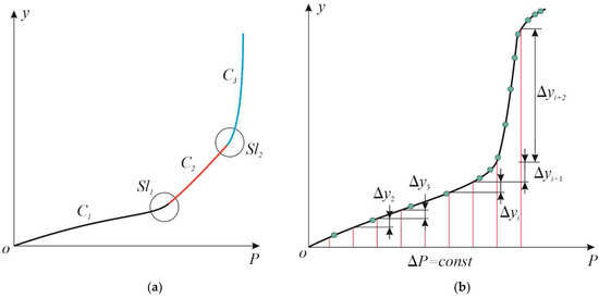
Figure 4.
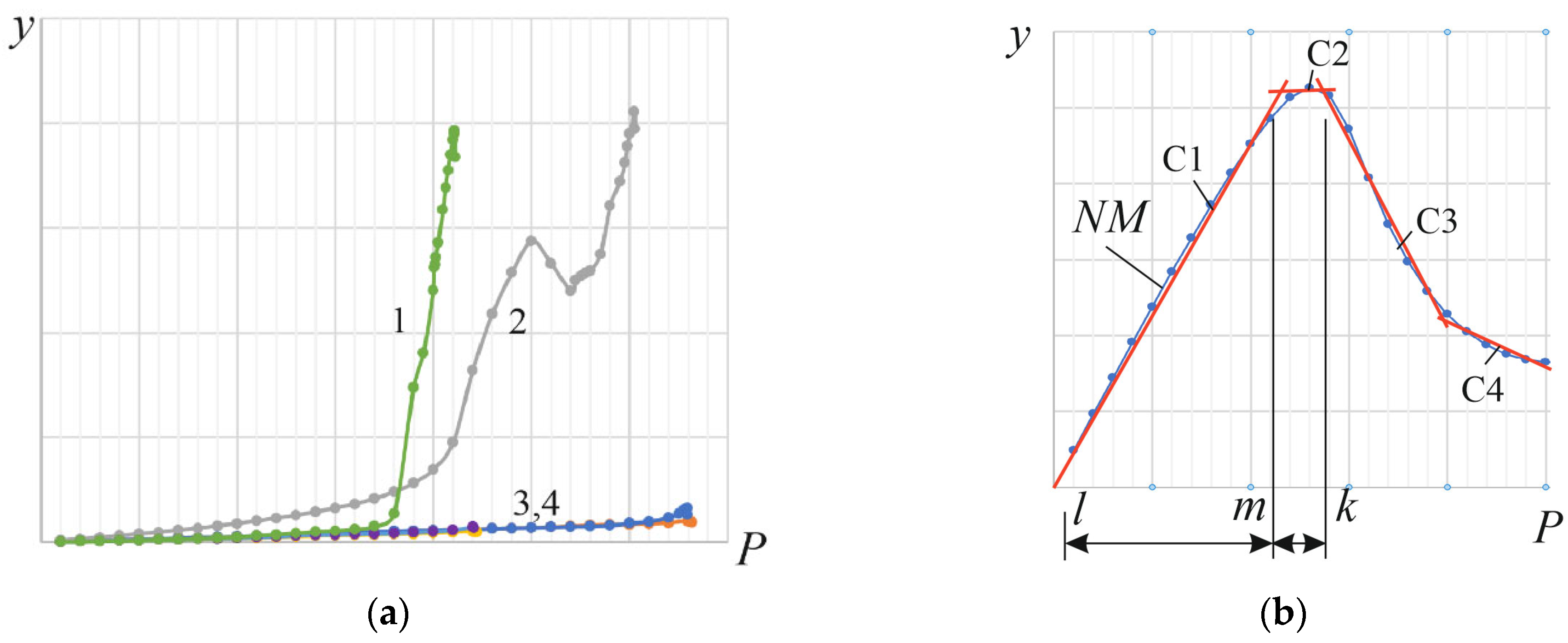
Geometric interpretation of stability loss of an element: topology of dependence of displacement y on load P (a): C1–C3 are curve segments between the knees; Sl1, Sl2 are curve knees; scheme to calculate decreasing rates for the function y(P) (b).
The co-deformation of structural elements in buildings of this type demonstrates that, in many special cases, the force–displacement dependence has near-linear segments (Figure 4a) and nonlinear segments in the knee zones . Computations show that the presence of these nonlinear segments accelerates the rate of displacements in case of a uniform increase in loading. However, Figure 4b shows that this rate hardly changes: for linear segments.
A knee segment can demonstrate an increase by double or even more in displacements. Therefore, the following criterion can be considered as a condition for loss of stability:
where is the number of the loading step featuring an identical rate of increase and is the number of knee segments, taken as being equal to one in the first case of satisfaction of Condition (3). This number increases by one in each subsequent case of satisfaction of this condition. Additionally, 2 is the coefficient taking into account the effect of minor nonlinearity on the quasi-linear segment of a curve, for example, curve in Figure 4a. The inequation on the right means that the material does not fail due to loss of strength.
If displacements at further steps are next to the first knee segment, then this case can be interpreted as the overall loss of stability of an element. If this condition is not met next to the knee segment, segment is the case, and the subsequent strain there can cause the second knee segment . In this case, segment can be interpreted as the local loss of stability (local buckling). can represent the loss of the bearing capacity of a structure.
In machine learning, the following algorithm can be used to identify the limit state:
- -
- Training data are labeled to identify the points belonging to segments , , of the stress–strain curve (see Figure 4a). The creation of arrays of point numbers between the knees of segments ; ; will suffice for this purpose.
- -
- Conditions should be checked and a conclusion should be made in accordance with Table 1 when a test set or a projection is made for the characteristic point .

Table 1.
Limit state criteria used for machine learning purposes.
Table 1.
Limit state criteria used for machine learning purposes.
| The Antecedent: Input Data | The Consequent: The Limit State |
|---|---|
| No limit state; serviceability | |
| Loss of strength or local loss of stability | |
| Loss of serviceability or local loss of stability with displacement restraints | |
| Loss of overall stability or loss of strength | |
2.2. Finite Element Modeling of a Structure
2.2.1. Finite Element Mesh, Loading, and Supports
The geometry of the facility was created using the SolidWorks 2020 software package and imported into the Siemcenter Femap 2021.1 system, where the structural elements remained unchanged (IFC format). The finite element model is shown in Figure 5a.
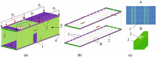
Figure 5.
Finite element model of a modular block, including load topology and bracings (a); discretization of frame elements (b); mesh fragments (c); 1, 2 are 4-node plate elements of the corrugated web and contour beams, respectively; 3 represents RBE2 elements, 4 represents pinned nodal constraints.
Elements of the corrugated web, top, and floor were broken into four-node shell elements, with the basic size of an element equaling 0.02 m. The following discretization method was used for rods (Figure 5b). Shell elements were used to simulate contour beams and lintels above openings; their actual dimensions and the shape of the cross-section were taken into account. Racks, girders, struts, and roof support beams were described using spatial rods, and the basic size of each spatial rod was also assumed to be 0.02 m. The levels of detail of the rod elements were introduced to take into account the local compression and loss of stability for cases of ultimate loading. All nodal joints, except for block fittings, were assumed to be welded. The contact between rod elements and plates was taken into account by introducing RBE2 elements (Figure 5c), which stiffly connected an independent node of a rod to dependent nodes of the cross-section. Two independent loads and , shown in Figure 5a, were used for the structural analysis. This type of loading was chosen in order to take into account supplementary structures and equipment items to be placed above. The maximum values of these loads were analyzed, and they corresponded to the ultimate loading conditions specified in Table 1.
2.2.2. Description of the Structural Analysis Method
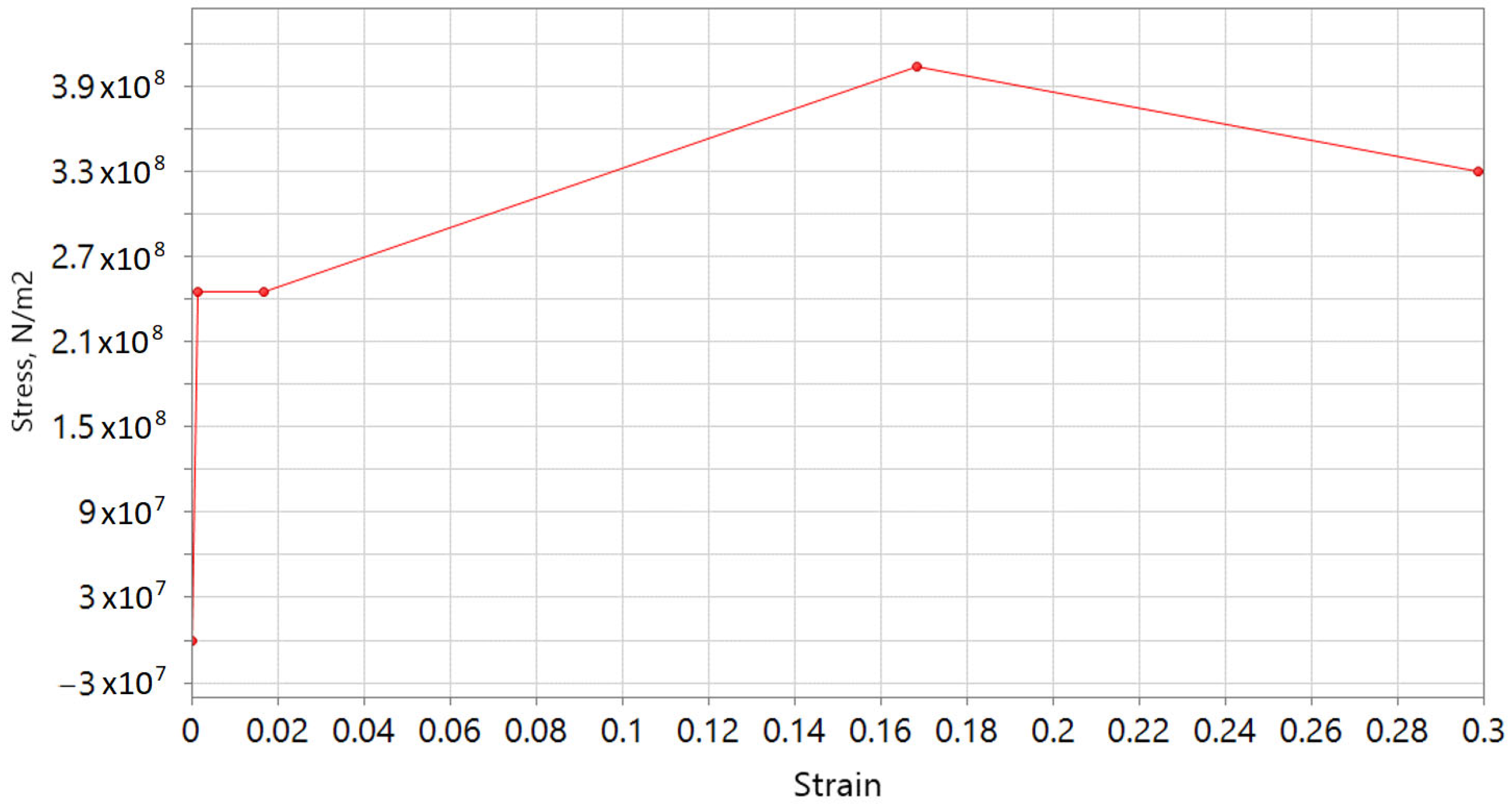
The finite element method was used to perform a structural analysis on the static formulation. Physical and geometrical nonlinearities were taken into account. Von Mises equivalent stresses and strains were used to analyze the stress–strain state. The strains in steel rod elements were simulated using the diagram provided in Figure 6, which shows positive values of stresses and strains; this diagram is mirror-symmetric for negative values. Stress values are provided for the C255 steel used in the computations. The following equation was used to take into account physical and geometrical nonlinearities:
where is the tangent stiffness matrix; is the displacement vector, computed at iteration for nodes of the finite element model; and is the load vector transformed into nodal forces. The vector is drawn randomly; it consists of a system of nodal forces in the state of static equilibrium.
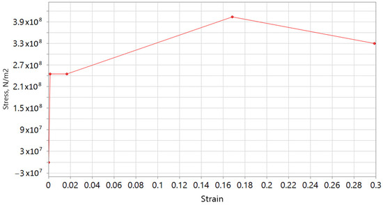
Figure 6.
Strain diagram.
Small values of forces are set for this vector to avoid any effect on the solution if the load values are far from the critical one, causing a loss of stability. Forces should be set in such a way that the displacements they cause can reproduce the projected buckling pattern of structural elements.
The tangent stiffness matrix is formulated as follows:
where is a tangent matrix whose elasticity coefficients take account of the strain diagram (Figure 6); is a geometric matrix determined by the vector of longitudinal forces computed at iteration . The Newton–Raphson method was used to solve the nonlinear problem with a force bias of 0.001. The value of the acting load was applied stepwise; 1/40 of the full value of loads was applied at each step. It took no more than 25 iterations to check the convergence of the iterative process at each step of loading.
2.3. Machine Learning Models
2.3.1. Making Regression Equations and Adapting Them for Modular Blocks
If the number of data points in a modular block does not exceed fifteen, the machine learning process has the following steps:
- -
- Making a linear regression equation.
- -
- Selecting the most effective metric to evaluate the accuracy of predictions.
- -
- Making a numerical model of a facility. In this case, the level of detail in a computational model and the modeling of various nonlinear effects should be taken into account. If the results of numerical modeling show strong nonlinear effects, the basic regression equation should be reconsidered and a higher-order polynomial should be chosen instead of a linear equation.
- -
- Making training and test sets. The size of the training set equals 70% of the total amount of data; the remaining data can be used for cross-validation on the test set.
- -
- Using selected metrics for the accurate evaluation of model predictions.
Basic regression equations. A standard equation of linear regression is used to predict the stress–strain state of a modular building:
where is the predicted von Mises strain value , scaled using the factor; is the vector of weight coefficients identified at the training stage; is the value of actual loading; and is the corrugated web thickness value at a characteristic observation point for which strains are determined.
It is noteworthy that Equation (6) can be applied to linear segments of strain diagrams made using numerical modeling. In the case of strongly nonlinear segments of diagrams, one can employ piecewise linear decomposition (Section 2.3.2) or use the following equation:
where is the Heaviside function; if the values of the argument , which is considered positive depending on the range that the value of enters; and is the number of ranges under consideration, Figure 7.
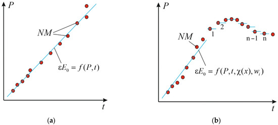
Figure 7.
Interpretation of model prediction made in the form of linear regression for linear data distribution (a) and for nonlinear data distribution (b).
It is assumed that Model (6) makes a satisfactorily accurate prediction if the condition of the minimum mean square deviation is satisfied:
where represents the values of relative von Mises strains at the point , obtained using numerical simulation; represents the values of strains at this point predicted using Equation (6); and Nq is the size of the test set.
The parameter matrix is introduced to solve the extremum Problem (8); this matrix is made using Equation (6) and the matrix notation for MSE:
where is the vector of weight coefficients. If the condition is true, it is sufficient to take the matrix derivative of the MSE matrix form Equation (9) with respect to and equate it to zero in order to find the accurate solution for . The following expression is obtained if simple transformations are omitted:
In case there is no inverse matrix for the matrix , the approximate solution to Problem (8) should be found using deterministic or stochastic search optimization methods.
2.3.2. Piecewise Linear Decomposition
Graphs describing dependence between the components of the stress–strain state can have intricate shapes, including several quasi-linear segments (Figure 8a).
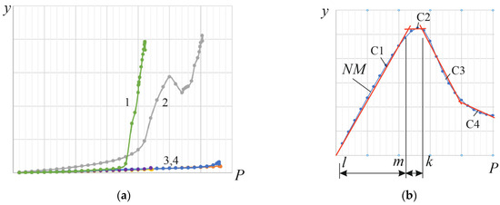
Figure 8.
Approximation of nonlinear functions: cases of dependence between displacement y and force P triggered by strain in steel structures: 1–4 numbers of possible dependencies (a); problem decomposition made to describe the nonlinear dependence NM by straight lines C1–C4; l, m, k are limits of ranges of p values (b).
In this case, an individual linear regression equation can be used for each range of values of a variable parameter. It is also necessary to divide the training sets accordingly. Then, the value of the function shown in Figure 8b (for example, for equivalent stress) for the segment can be described by the following expression:
In Figure 8b, an atypical, but more general, load–deflection curve is shown. The line C2 approximately describes the strengthening of the element before the failure of other elements in the system. The decrease in displacement values (lines C3, C4) was associated with the failure of another element in the system, which halted the load transfer, and part of the system became geometrically variable (a plastic hinge or a system of plastic hinges formed). Then, the system started to deform in such a way that the deflections changed their direction.
2.3.3. Development of Tree-Based Ensemble Methods
Computations of modular steel structures with a corrugated web show that the presence of this web greatly affects the load-bearing capacity. Moreover, different web thickness values translate into a unique set of characteristic points for the structure as a whole. Limit states are observed at these points. Hence, an ensemble system (Figure 9) is constructed using decision trees, each of which is associated with a unique corrugated web thickness value and its design resistance.
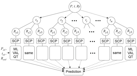
Figure 9.
Structure of the ensemble of decision trees: SCP is a set of critical points; ML is a machine learning block; VAL is a validation block; QT is the quality testing procedure.
Let us describe the system shown in Figure 9 in more detail. The initial data used to make the prediction needed to evaluate the stress–strain state that determines the serviceability or safety of a modular building (a container) are the values of the acting force; corrugated web thickness; and design resistance (), respectively. Tasks are decomposed depending on the thickness of the corrugated web. Each resulting task is a decision tree with initial leaves . Further, a system of critical points is made for each value of the design resistance of a corrugated web. The number of critical points is equal to . These points are determined for structural elements of a modular building in which the limit states, specified in Table 1, are reached.
Machine learning, including validation and quality evaluation, is performed for each point. Meanwhile, the following system of standard regression equations is made for a container as a whole:
where is a predictable hazard factor of the limit state at point on line segment 1 (please refer to Figure 8b, where this line is labeled as C1), which can be assumed as the equivalent von Mises stress, as equivalent strains or their scaled values, and as a resulting linear or angular displacement of a node. Here, indices are the number of straight lines approximating the dependence of the hazard factor on the load for the point , and is the same, but for the point .
When validation is performed, the following ratios of data amounts are used: the training set and the test set make up approximately 0.7 of the total amount of data; 0.3 of these data are used to make a prediction. To evaluate the quality of machine learning model values, MSE metrics are used as follows:
where is the size of the test set; is the limit state hazard factor identified as a result of model training; is the same for prediction; and is a set of line numbers approximating the nonlinear dependences of the value on the load .
Depending on the problem statement, Equation (7) can be used instead of standard regression equations. In this case, there is no need for approximation by linear functions, but it is noteworthy that this equation does not guarantee an acceptable result for all types of functions.
3. Results
3.1. Algorithm of Data Preparation for Machine Learning
To implement the proposed method, let us describe the main stages of data preparation using the case of a modular building block with internal welded nodes. The task is to predict the limit value of the load in accordance with the loading scheme shown in Figure 5a. The thickness of the corrugated web is the main parameter affecting the value of this load, together with the stiffness of the frame. The following steps are needed to obtain the data required for the study:
- -
- Making sets of corrugated web thicknesses (see Figure 9, Table 2) for which training data must be obtained. It is reasonable to use standard thickness products manufactured by metal smelters. The following thicknesses are taken as a set of available values in accordance with the standards, in mm: Other design parameters can be adopted considering the structural requirements and design experience of the modular constructions under consideration.
- -
- Making a computation in a physically nonlinear formulation and extracting data at each pre-set loading step (forming the set on Figure 9) for each thickness value in question, or selecting a limit state hazard factor, for example, von Mises strain values or their scaled values . Scaling is sometimes necessary to reduce the absolute values of weights in regression equations. The criteria for reaching the limit state are taken from Table 1. In this case, if the operational requirements assume that the system deforms elastically, von Mises stress values or deflection values can be used.
- -
- Sorting load values in the ascending order according to loading stages; selecting and filling the matrix ; and checking the existence of the inverse matrix and the strength of its causation using an infinite norm required for a stable solution to the system of the equation (Equation (10)).
- -
- Performing the transformations (Equation (10)) to obtain the weight coefficients and formulating Equation (12) consisting of the equations for the points (Equation (11)).
- -
- Generating a sample and validating the ensemble model using Expression (13) or other known quality metrics.
Table 2.
Demonstration dataset for a training set at point A.
Table 2.
Demonstration dataset for a training set at point A.
| № | kN | Strain | kN | Strain | kN | Strain | |||
|---|---|---|---|---|---|---|---|---|---|
| mm | mm | mm | |||||||
| 1 | 100 | 2.98 × 10⁻⁵ | 5.967928 | 100 | 3.05 × 10⁻⁵ | 6.108622 | 100 | 3.14 × 10⁻⁵ | 6.276434 |
| 2 | 200 | 5.96 × 10⁻⁵ | 11.92611 | 200 | 6.1 × 10⁻⁵ | 12.20766 | 200 | 6.27 × 10⁻⁵ | 12.54381 |
| 3 | 300 | 8.94 × 10⁻⁵ | 17.87428 | 300 | 9.15 × 10⁻⁵ | 18.29604 | 300 | 9.4 × 10⁻⁵ | 18.80007 |
| 4 | 400 | 0.000119 | 23.81122 | 400 | 0.000122 | 24.37342 | 400 | 0.000125 | 25.0453 |
| 5 | 500 | 0.000149 | 29.73724 | 500 | 0.000152 | 30.43934 | 500 | 0.000156 | 31.27862 |
| 6 | 600 | 0.000178 | 35.65146 | 600 | 0.000182 | 36.49368 | 600 | 0.000188 | 37.50006 |
| 7 | 700 | 0.000208 | 41.55344 | 700 | 0.000213 | 42.53462 | 700 | 0.000219 | 43.70862 |
| 8 | 800 | 0.000237 | 47.44258 | 800 | 0.000243 | 48.56278 | 800 | 0.00025 | 49.90342 |
| 9 | 900 | 0.000267 | 53.31846 | 900 | 0.000273 | 54.57748 | 900 | 0.00028 | 56.08418 |
| 10 | 1000 | 0.000296 | 59.18018 | 1000 | 0.000303 | 60.57726 | 1000 | 0.000311 | 62.24974 |
| 11 | 1100 | 0.000325 | 65.02728 | 1100 | 0.000333 | 66.56232 | 1100 | 0.000342 | 68.4007 |
| 12 | 1200 | 0.000354 | 70.85904 | 1200 | 0.000363 | 72.53132 | 1200 | 0.000373 | 74.53524 |
| 13 | 1300 | 0.000383 | 76.67696 | 1300 | 0.000392 | 78.48694 | 1300 | 0.000403 | 80.65636 |
| 14 | 1400 | 0.000412 | 82.48218 | 1400 | 0.000422 | 84.42982 | 1400 | 0.000434 | 86.76536 |
| 15 | 1500 | 0.000441 | 88.27358 | 1500 | 0.000452 | 90.3577 | 1500 | 0.000464 | 92.85828 |
| 16 | 1600 | 0.00047 | 94.04914 | 1600 | 0.000481 | 96.26996 | 1600 | 0.000495 | 98.93764 |
| 17 | 1700 | 0.000499 | 99.8047 | 1700 | 0.000511 | 102.1632 | 1700 | 0.000525 | 105.0034 |
| 18 | 1800 | 0.000528 | 105.5374 | 1800 | 0.00054 | 108.0404 | 1800 | 0.000555 | 111.0493 |
| 19 | 1900 | 0.000556 | 111.2549 | 1900 | 0.000569 | 113.8913 | 1900 | 0.000585 | 117.0601 |
| 20 | 2000 | 0.000585 | 116.9439 | 2000 | 0.000599 | 119.7122 | 2000 | 0.000615 | 123.0384 |
| 21 | 2100 | 0.000613 | 122.6044 | 2100 | 0.000628 | 125.5025 | 2100 | 0.000645 | 128.9855 |
| 22 | 2200 | 0.000641 | 128.2351 | 2200 | 0.000656 | 131.2569 | 2200 | 0.000674 | 134.8774 |
| 23 | 2300 | 0.000669 | 133.7948 | 2300 | 0.000685 | 136.9114 | 2300 | 0.000703 | 140.6381 |
| 24 | 2400 | 0.000696 | 139.2214 | 2400 | 0.000712 | 142.4451 | 2400 | 0.000731 | 146.2874 |
| 25 | 2500 | 0.000723 | 144.5645 | 2500 | 0.000739 | 147.8557 | 2500 | 0.000759 | 151.7854 |
| 26 | 2600 | 0.000749 | 149.7023 | 2600 | 0.000765 | 153.0923 | 2600 | 0.000788 | 157.5254 |
| 27 | 2700 | 0.000774 | 154.7916 | 2700 | 0.000797 | 159.4357 | 2700 | 0.00085 | 170.0867 |
| 28 | 2800 | 0.000817 | 163.3491 | 2800 | 0.000872 | 174.3546 | 2725 | 0.000876 | 175.2371 |
| 29 | 2900 | 0.000892 | 178.4938 | 2900 | 0.000963 | 192.6884 | 2750 | 0.000902 | 180.3507 |
| 30 | 3000 | 0.000978 | 195.6542 | 3000 | 0.001064 | 212.8616 | 2775 | 0.000922 | 184.3269 |
| 31 | 3100 | 0.001066 | 213.224 | 3100 | 0.001167 | 233.3186 | 2800 | 0.000942 | 188.3637 |
| 32 | 3200 | 0.001141 | 228.178 | 3200 | 0.00126 | 251.9048 | 2850 | 0.001003 | 200.5564 |
| 33 | 3300 | 0.001169 | 233.8726 | 3250 | 0.001285 | 257.0694 | 2900 | 0.001049 | 209.8774 |
| 34 | 3312.5 | 0.001147 | 229.3522 | 3275 | 0.001284 | 256.8072 | 2950 | 0.001118 | 223.6064 |
3.2. Case of Value Prediction for a Nonlinear Function
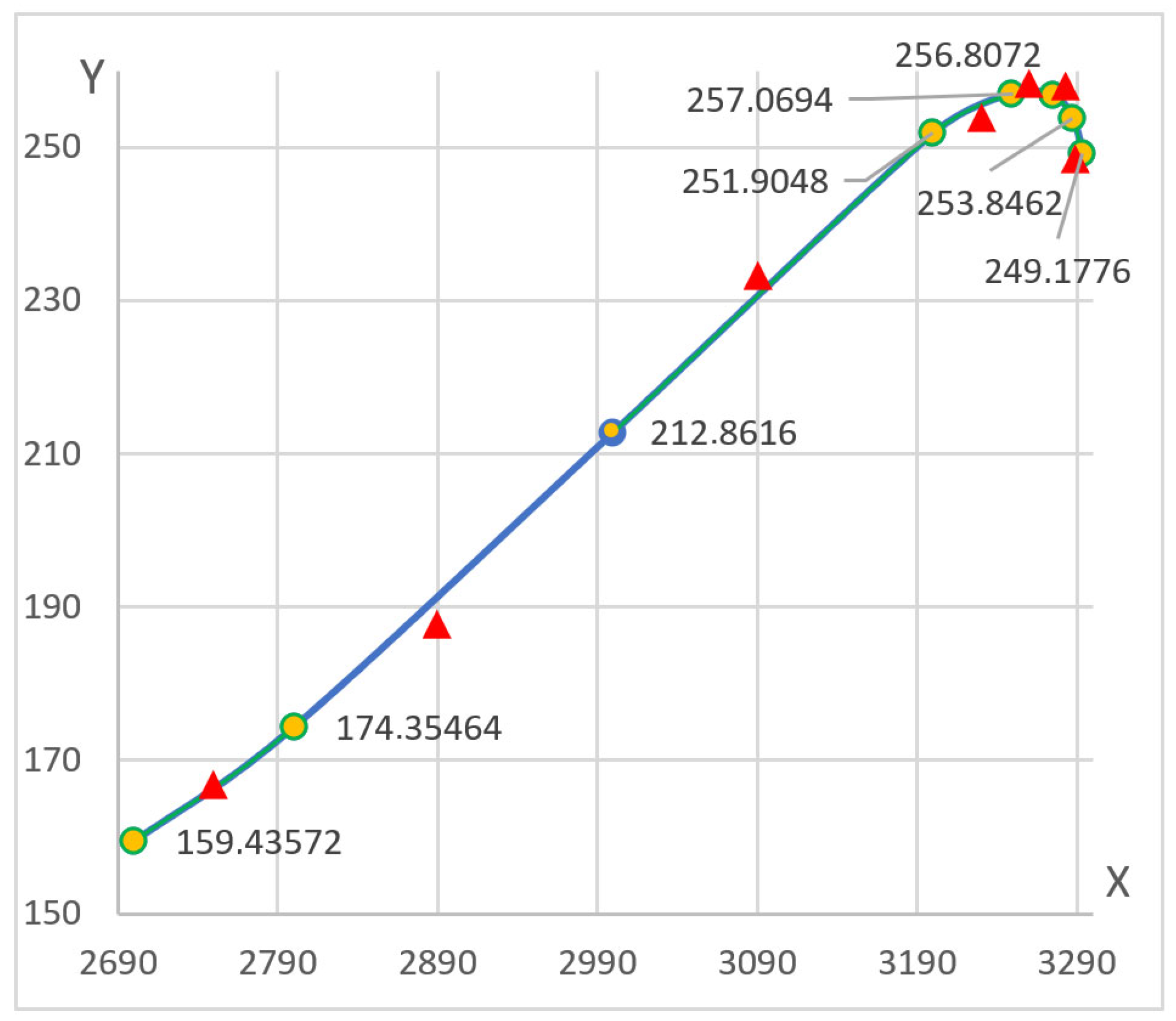
Before predicting the stress–strain state (SSS) of a real structure, let us consider the model performance using the nonlinear function , shown as a continuous curve in Figure 10.
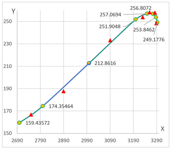
Figure 10.
Nonlinear function and results of its matrix approximation.
Let us select several points, marked by circles on the curve, in order to train the model. The data vector , used for training purposes, will consist of the function values shown in the figure. We will use Equation (7) to take into account nonlinearity, then add features to the matrix in order to take into account the nonlinear nature of this function. The matrix will be as follows:
The following result can be obtained according to Equation (10):
Hence,
This vector is used to find values at the intermediate points, which are shown in Figure 10 as red triangles. When these values are computed, the presence of non-linear features in the matrix should be taken into account. For example, to obtain the value y = f(2750), the vector of the initial data will be as follows: . There are no nonlinear features there, and for y = f(3260), . The figure shows that this training method is used to quite accurately predict the values of the function without knowing its analytical formulation. Let us compute the prediction quality metric using Formula (8). The result is , which is acceptable for the selected size of the training set and the target variable varying in the range . The standardized value of is the coefficient of determination: 0.89. This means that the model makes satisfactory predictions.
3.3. Case of Model Training and Verification of the Web Thickness of a Steel Block of a Modular Building for a Pre-Set Load Value
In general, the process of training and predicting parameters for a modular building block is implemented according to the scheme shown in Figure 9. FEM computations show that the thickness of a corrugated web is the decisive factor for the ultimate load value . Limit states are reached at one of the three points shown in Figure 11 for this type of load and any of the thickness values considered here. A predictive model is made for point A as an example.
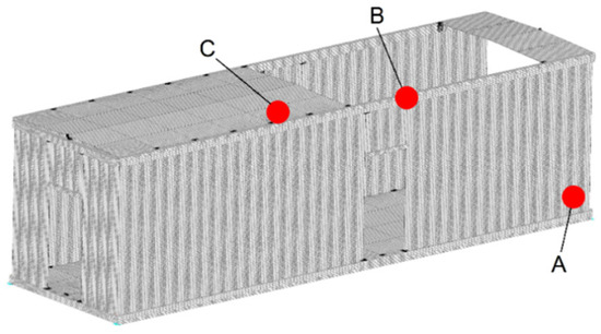
Figure 11.
Characteristic set (A, B, C) of points describing the stress–strain state of a structure.
Let us take a closer look at the decision tree with the following fixed parameters: MPa, mm, mm, and mm. The finite element method is applied to generate the training data arranged in ascending order of loading. The track record of matrix generation for various facilities shows that scaling factors or regularization must be applied to the training data to generate a well-conditioned matrix.
The data prepared for training purposes are presented in Table 2. Data ranges used within the concept of decomposition are colored (see Figure 8b). The yellow color highlights the data describing the first curve; the orange color highlights the data describing the second curve. The values of equivalent von Mises strains are multiplied by the scaling factor that equals . For simplicity purposes, if the block length is 12 m, the total load acting on the system (see Figure 5a) is represented by the load parameter which is the equivalent force .
The ranges of load values (provided in Table 2 above), including for all thicknesses and ranges , , and for thicknesses , , and , are used to make matrices , , , , and and to find weight coefficients . These matrices are not provided here because they are too cumbersome. Below are the final regression equations for point A. These equations are needed to find values of von Mises strains using the initial data provided in the form of generalized load and thickness values:
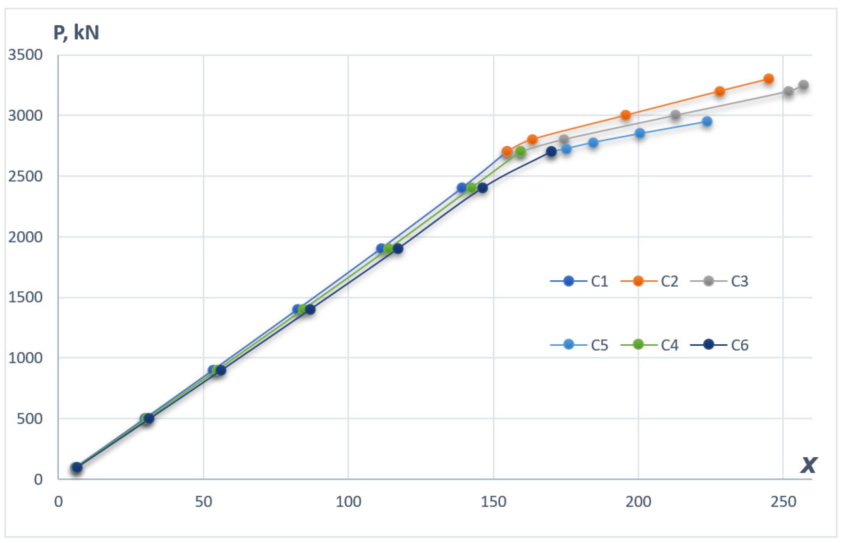
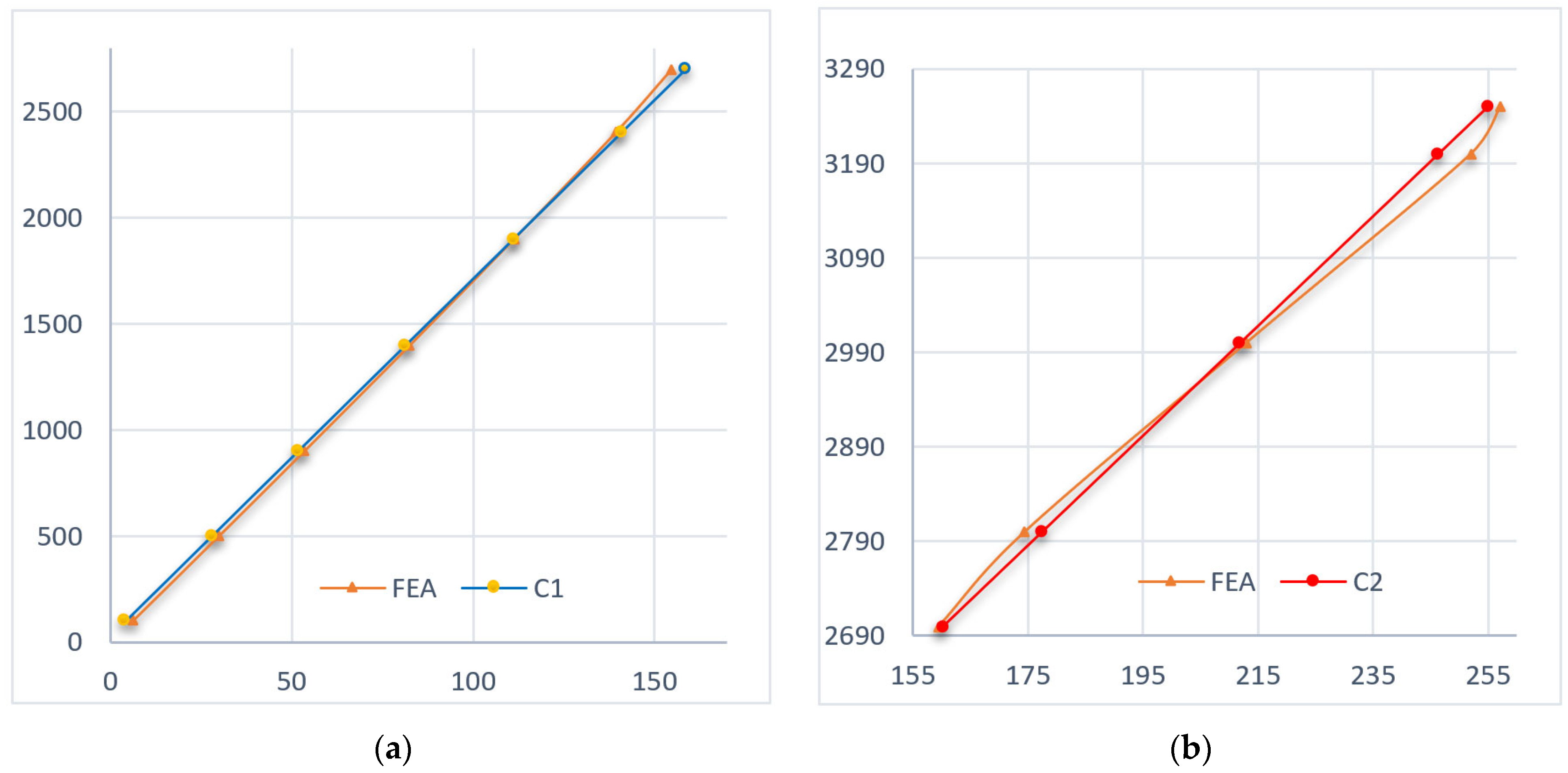
The computation results obtained from Equation (14) for thicknesses , , and and different values of the load parameter P are illustrated in Figure 12.
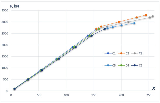
Figure 12.
Curves describing scaled strains x = εE0 at point A for different thickness values of the corrugated web obtained by machine learning: C1, C2 for the 3 mm thickness; C3, C4 for the 2.5 mm thickness; C5, C6 for the 2 mm thickness.
These projection data were compared with the nonlinear FEM computation, which confirmed the acceptable accuracy of the projections. Figure 13 shows data curves C1 and C2 compared with the nonlinear FEM computation (Figure 13).
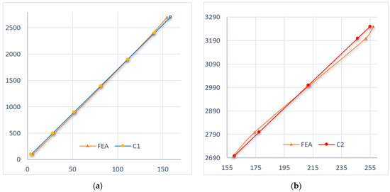
The quality of the predictions, evaluated using the MSE metric (8), is as follows: for Equation (1) of the system (14), MPa and the coefficient of determination is 0.92; for Equation (2) of the system (14), MPa and 0.88. These values confirm the successful model validation of the test sets.
Systems of equations are made for points B and C in a similar way, depending on the stress–strain curve plotted at the training stage. A system of equations (Equation (14)) whose curve has knees will contain three rather than two equations. This allows the machine learning model to identify the local loss of stability of structural elements in accordance with criterion (3). Further, the systems of Equation (14) are assembled into an ensemble in accordance with Figure 9 and Expression (12), which makes it possible to predict the stress–strain state of a modular block for different steel grades and options of SCP (sets of critical points) determined by different variants of loading.
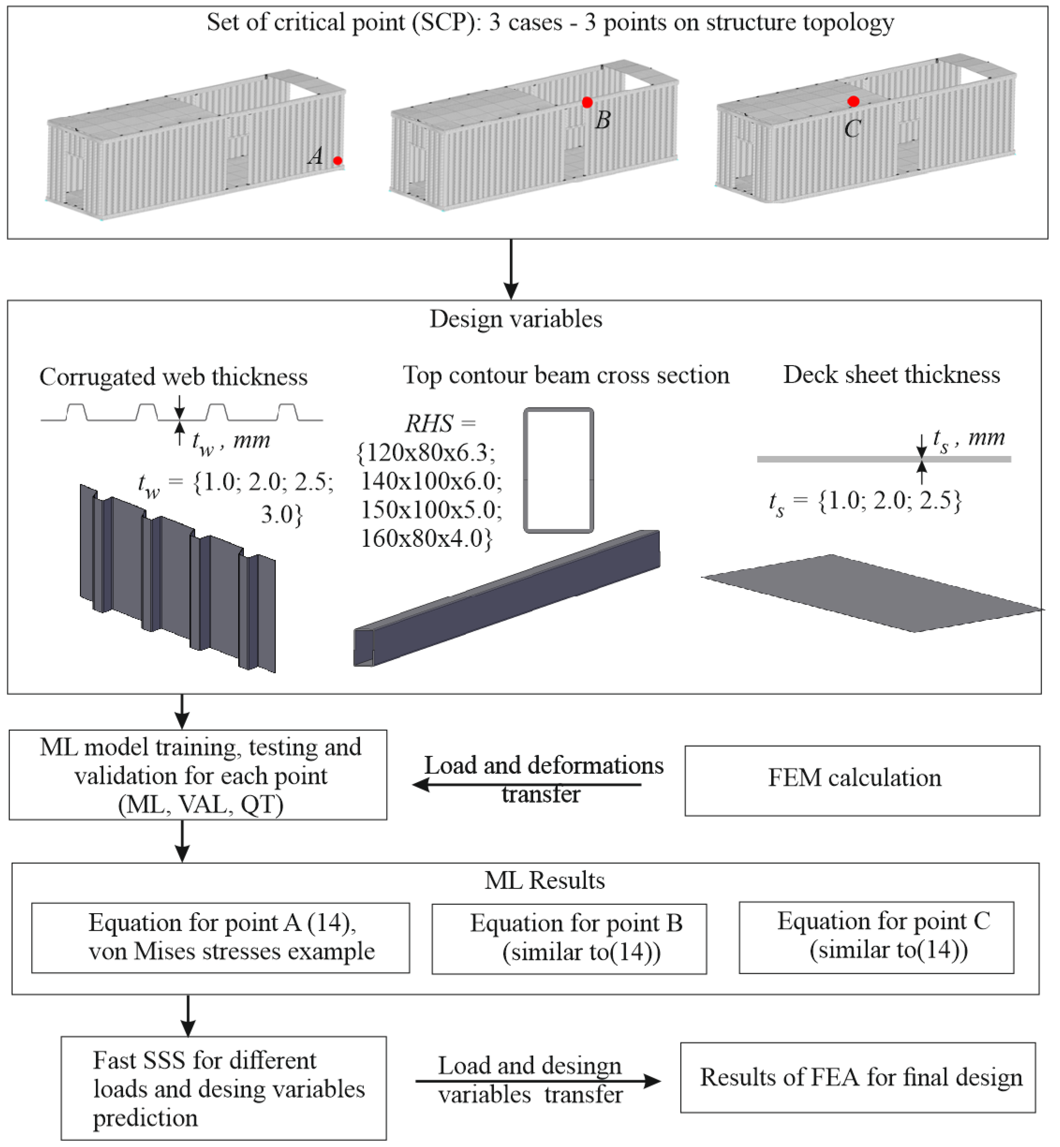
The general scheme for obtaining a design solution for one of the decision trees formed according to Figure 9 is shown in Figure 14. Let us explain this figure. In the case of designing a modular block, the task is to find the maximum load while minimizing the cost of the object. For the formed SCP, as a result of preliminary finite element analysis, design variables are determined. In this case, they consist of the thicknesses of sheets and profiles of the cross-sections of rod elements. Then, for each point from the SCP, regression equations are constructed to predict the components of the stress–strain state (SSS). As an example, the construction of such equations is given in the article in the form of Equation (14) for normal stresses. As a result of using machine learning, a system of equations is obtained, which facilitates the selection of design parameters (thicknesses of sheets and rod profiles) for a given load value, taking into account the minimization of material consumption. It should be noted that the prediction results cannot be used as the final solution. The obtained forecast should be verified by calculation using the finite element method or other validated methods. In this case, to solve the minimization problem using the brute-force method without machine learning, it is necessary to perform 96 labor-intensive FEM calculations, which requires a significant amount of time for the engineer.

Figure 14.
Design procedure for a modular building considering the minimization of its material consumption.
4. Discussion
More detailed predictions of the stress–strain states of structures require a larger number of characteristic points where a limit state is likely to occur. In this case, the system of equations (Equation (10)) may remain unsolved because of poor conditioning or the impossibility of inversion of the matrix . If this is the case, Problem (8) can be solved using the gradient descent method or similar gradient methods. If the matrix has 10-30 parameters, then genetic algorithms such as those described in [47,48] can be effectively used. These algorithms have an optimization objective explicitly formulated as Formula (8), while the variable parameters are weights represented as discrete sets of values with small steps. Methods of swarm intelligence can also be employed, including firefly, ant colony, gray wolf algorithms, etc.
Nonlinear computations made for modular construction facilities, consisting of a large number of blocks, are very labor-intensive. Hence, the direct learning process is constrained by the computational capacity of the computer. Therefore, to reduce the amount of computation, a rod structure can replace a plate enclosure structure [49]. However, this operation requires supplementary substantiation and may adversely affect the prediction results.
Machine learning models use linear regression equations in a number of cases, although the processes for which predictions are made are nonlinear. The correct operation of such models requires the training data to be prepared in a special way. For example, supplementary features should be added to the matrix in accordance with Equation (7), and regularization of regression equations should be applied. These processes require supplementary data in order to train and adjust the model parameters. Therefore, it is reasonable to consider the use of nonlinear regression equations, for example, power polynomials. However, in this case, the feature matrix, which is needed to make accurate projections, may be very large.
5. Conclusions
- A new approach to evaluating strains in steel modular blocks with corrugated webs is proposed in the article. This approach is based on machine learning and takes into account the deterministic identification of weight coefficients. The novel approach encompasses:
- -
- The principle of decomposing strain curves into rectilinear segments and training models as connected piecewise linear functions;
- -
- Taking into account strain diagrams for structural elements by means of modification (binarization) of the feature matrix if the principle of decomposition can hardly be applied;
- -
- Developing an ensemble learning model on the basis of a set of decision trees; this model can greatly expand the prediction domain for changing design parameters.
- A simple deterministic approach to identifying model weight coefficients is found to be effective for a steel modular block. This approach is based on finding the minimum discrepancy between predicted and reference values using matrix derivatives. This approach does not require any time-consuming gradient or stochastic methods. However, this approach requires a special preparation of training data to obtain well-conditioned feature matrices.
- Models demonstrate high degrees of confidence in predictions evaluated by relevant quality metrics. For example, the coefficient of determination R2 for all ensemble models is not below 0.88, while the MSE metric also shows very low values.
- The proposed ensemble learning method can be recommended as an instrument for evaluating the stress–strain states of steel frame and truss structures subjected to natural or anthropogenic emergency effects in order to predict the terms of their safe operation, as well as their resistance to progressive collapse.
Author Contributions
Conceptualization, A.V.A.; Methodology, A.R.T. and A.V.A.; Software, A.V.A.; Formal analysis, A.R.T.; Investigation, A.V.A. and O.T.; Data curation, O.T.; Writing—original draft, O.T. All authors have read and agreed to the published version of the manuscript.
Funding
The research was funded by the National Research Moscow State University of Civil Engineering (grant for fundamental and applied scientific research, project No. 04-234/130).
Data Availability Statement
The original contributions presented in the study are included in the article, further inquiries can be directed to the corresponding author.
Conflicts of Interest
The authors declare no conflict of interest.
References
- Faludi, J.; Lepech, M.D.; Loisos, G. Using Life Cycle Assessment Methods to Guide Architectural Decision-Making for Sustainable Prefabricated Modular Buildings. J. Green. Build. 2012, 7, 151–170. [Google Scholar] [CrossRef]
- Wang, Z.; Tsavdaridis, K.D. Optimality Criteria-Based Minimum-Weight Design Method for Modular Building Systems Subjected to Generalised Stiffness Constraints: A Comparative Study. Eng. Struct. 2022, 251, 113472. [Google Scholar] [CrossRef]
- Gatheeshgar, P.; Poologanathan, K.; Gunalan, S.; Shyha, I.; Sherlock, P.; Rajanayagam, H.; Nagaratnam, B. Development of Affordable Steel-Framed Modular Buildings for Emergency Situations (COVID-19). Structures 2021, 31, 862–875. [Google Scholar] [CrossRef]
- Wang, Z.; Rajana, K.; Corfar, D.A.; Tsavdaridis, K.D. Automated Minimum-Weight Sizing Design Framework for Tall Self-Standing Modular Buildings Subjected to Multiple Performance Constraints under Static and Dynamic Wind Loads. Eng. Struct. 2023, 286, 116121. [Google Scholar] [CrossRef]
- Ferdous, W.; Bai, Y.; Ngo, T.D.; Manalo, A.; Mendis, P. New Advancements, Challenges and Opportunities of Multi-Storey Modular Buildings–A State-of-the-Art Review. Eng. Struct. 2019, 183, 883–893. [Google Scholar] [CrossRef]
- Benjamin, S.; Christopher, R.; Carl, H. Feature Modeling for Configurable and Adaptable Modular Buildings. Adv. Eng. Inform. 2022, 51, 101514. [Google Scholar] [CrossRef]
- Gan, V.J.L. BIM-Based Graph Data Model for Automatic Generative Design of Modular Buildings. Autom. Constr. 2022, 134, 104062. [Google Scholar] [CrossRef]
- Munmulla, T.; Navaratnam, S.; Hidallana-Gamage, H.D.; Tushar, Q.; Ponnampalam, T.; Zhang, G.; Jayasinghe, M.T.R. Sustainable Approaches to Improve the Resilience of Modular Buildings under Wind Loads. J. Constr. Steel Res. 2023, 211, 108124. [Google Scholar] [CrossRef]
- Luo, F.J.; Bai, Y.; Hou, J.; Huang, Y. Progressive Collapse Analysis and Structural Robustness of Steel-Framed Modular Buildings. Eng. Fail. Anal. 2019, 104, 643–656. [Google Scholar] [CrossRef]
- Chen, Z.; Zhong, X.; Liu, Y.; Liu, J. Analytical and Design Method for the Global Stability of Modular Steel Buildings. Int. J. Steel Struct. 2021, 21, 1741–1758. [Google Scholar] [CrossRef]
- Zhong, X.; Chen, Z.; Liu, J.; Liu, Y. Numerical Simulations to Explore the In-Plane Performance of Discontinuous Diaphragms in Modular Steel Buildings. Thin-Walled Struct. 2023, 188, 110810. [Google Scholar] [CrossRef]
- Farajian, M.; Sharafi, P.; Bigdeli, A.; Eslamnia, H.; Rahnamayiezekavat, P. Experimental Study on the Natural Dynamic Characteristics of Steel-Framed Modular Structures. Buildings 2022, 12, 587. [Google Scholar] [CrossRef]
- Srisangeerthanan, S.; Hashemi, M.J.; Rajeev, P.; Gad, E.; Fernando, S. Numerical Study on Performance Assessment of an Innovative Boltless Connection for Modular Building Construction. Thin-Walled Struct. 2023, 185, 110622. [Google Scholar] [CrossRef]
- Ping, T.; Pan, W.; Mou, B. An Innovative Type of Module-to-Core Wall Connections for High-Rise Steel Modular Buildings. J. Build. Eng. 2022, 62, 105425. [Google Scholar] [CrossRef]
- Lacey, A.W.; Chen, W.; Hao, H. Experimental Methods for Inter-Module Joints in Modular Building Structures—A State-of-the-Art Review. J. Build. Eng. 2022, 46, 103792. [Google Scholar] [CrossRef]
- Corfar, D.A.; Tsavdaridis, K.D. A Hybrid Inter-Module Connection for Steel Modular Building Systems with SMA and High-Damping Rubber Components. Eng. Struct. 2023, 289, 116281. [Google Scholar] [CrossRef]
- Ma, H.; Huang, Z.; Song, X.; Ling, Y. A Study on Mechanical Performance of an Innovative Modular Steel Building Connection with Cross-Shaped Plug-In Connector. Buildings 2023, 13, 2382. [Google Scholar] [CrossRef]
- Chen, Z.; Wang, J.; Liu, J.; Cong, Z. Tensile and Shear Performance of Rotary Inter-Module Connection for Modular Steel Buildings. J. Constr. Steel Res. 2020, 175, 106367. [Google Scholar] [CrossRef]
- Chen, H.L.; Ke, C.; Chen, C.; Li, G.Q. Study on the Shear Behavior of Inter-Module Connection with a Bolt and Shear Key Fitting for Modular Steel Buildings. Adv. Struct. Eng. 2023, 26, 218–233. [Google Scholar] [CrossRef]
- Sendanayake, S.V.; Thambiratnam, D.P.; Perera, N.J.; Chan, T.H.T.; Aghdamy, S. Enhancing the Lateral Performance of Modular Buildings through Innovative Inter-Modular Connections. Structures 2021, 29, 167–184. [Google Scholar] [CrossRef]
- Yang, C.; Xu, B.; Xia, J.; Chang, H.; Chen, X.; Ma, R. Mechanical Behaviors of Inter-Module Connections and Assembled Joints in Modular Steel Buildings: A Comprehensive Review. Buildings 2023, 13, 1727. [Google Scholar] [CrossRef]
- Thai, H.T.; Ho, Q.V.; Li, W.; Ngo, T. Progressive Collapse and Robustness of Modular High-Rise Buildings. Struct. Infrastruct. Eng. 2022, 19, 103977. [Google Scholar] [CrossRef]
- Peng, J.; Hou, C.; Shen, L. Progressive Collapse Analysis of Corner-Supported Composite Modular Buildings. J. Build. Eng. 2022, 48, 103977. [Google Scholar] [CrossRef]
- Munmulla, T.; Navaratnam, S.; Thamboo, J.; Ponnampalam, T.; Damruwan, H.G.H.; Tsavdaridis, K.D.; Zhang, G. Analyses of Structural Robustness of Prefabricated Modular Buildings: A Case Study on Mid-Rise Building Configurations. Buildings 2022, 12, 1289. [Google Scholar] [CrossRef]
- Ginigaddara, T.; Ekanayake, C.; Gunawardena, T.; Mendis, P. Resilience and Performance of Prefabricated Modular Buildings Against Natural Disasters. Electron. J. Struct. Eng. 2023, 23, 85–92. [Google Scholar] [CrossRef]
- Chua, Y.S.; Pang, S.D.; Liew, J.Y.R.; Dai, Z. Robustness of Inter-Module Connections and Steel Modular Buildings under Column Loss Scenarios. J. Build. Eng. 2022, 47, 103888. [Google Scholar] [CrossRef]
- Caçoilo, A.; Mourão, R.; Teixeira-Dias, F.; Lecompte, D. Pressure-Impulse Blast Response of Steel Iso-Containers. In Proceedings of the Internationational Symposium for the Interaction of Munitions with Structures, Panama City Beach, FL, USA, 21–25 October 2019. [Google Scholar]
- Yu, Y.; Tian, P.; Man, M.; Chen, Z.; Jiang, L.; Wei, B. Experimental and Numerical Studies on the Fire-Resistance Behaviors of Critical Walls and Columns in Modular Steel Buildings. J. Build. Eng. 2021, 44, 102964. [Google Scholar] [CrossRef]
- Hajirezaei, R.; Sharafi, P.; Kildashti, K.; Alembagheri, M. Robustness of Corner-Supported Modular Steel Buildings with Core Walls. Buildings 2024, 14, 235. [Google Scholar] [CrossRef]
- Alembagheri, M.; Sharafi, P.; Hajirezaei, R.; Tao, Z. Anti-Collapse Resistance Mechanisms in Corner-Supported Modular Steel Buildings. J. Constr. Steel Res. 2020, 170, 106083. [Google Scholar] [CrossRef]
- Pan, W.; Zhang, Z. Benchmarking the Sustainability of Concrete and Steel Modular Construction for Buildings in Urban Development. Sustain. Cities Soc. 2023, 90, 104400. [Google Scholar] [CrossRef]
- Peng, J.; Hou, C.; Shen, L. Numerical Analysis of Corner-Supported Composite Modular Buildings under Wind Actions. J. Constr. Steel Res. 2021, 187, 106942. [Google Scholar] [CrossRef]
- Generalova, E.M.; Generalov, V.P.; Kuznetsova, A.A. Modular Buildings in Modern Construction. Procedia Eng. 2016, 153, 167–172. [Google Scholar] [CrossRef]
- Dai, Z.; Cheong, T.Y.C.; Pang, S.D.; Liew, J.Y.R. Experimental Study of Grouted Sleeve Connections under Bending for Steel Modular Buildings. Eng. Struct. 2021, 243, 112614. [Google Scholar] [CrossRef]
- Lacey, A.W.; Chen, W.; Hao, H.; Bi, K. Structural Response of Modular Buildings–An Overview. J. Build. Eng. 2018, 16, 45–56. [Google Scholar] [CrossRef]
- Sharafi, P.; Mortazavi, M.; Samali, B.; Ronagh, H. Interlocking System for Enhancing the Integrity of Multi-Storey Modular Buildings. Autom. Constr. 2018, 85, 263–272. [Google Scholar] [CrossRef]
- Sun, Z.; Mei, H.; Pan, W.; Zhang, Z.; Shan, J. A Robotic Arm Based Design Method for Modular Building in Cold Region. Sustainability 2022, 14, 1452. [Google Scholar] [CrossRef]
- Chen, Z.; Wang, J.; Liu, J.; Khan, K. Seismic Behavior and Moment Transfer Capacity of an Innovative Self-Locking Inter-Module Connection for Modular Steel Building. Eng. Struct. 2021, 245, 112978. [Google Scholar] [CrossRef]
- Yang, N.; Xia, J.; Chang, H.; Zhang, L.; Yang, H. A Novel Plug-in Self-Locking Inter-Module Connection for Modular Steel Buildings. Thin-Walled Struct. 2023, 187, 110774. [Google Scholar] [CrossRef]
- Bertolini, M.; Guardigli, L. Upcycling Shipping Containers as Building Components: An Environmental Impact Assessment. Int. J. Life Cycle Assess. 2020, 25, 947–963. [Google Scholar] [CrossRef]
- Su, M.; Yang, B.; Wang, X. Research on Integrated Design of Modular Steel Structure Container Buildings Based on BIM. Adv. Civ. Eng. 2022, 2022, 1–13. [Google Scholar] [CrossRef]
- Fu, F. Fire Induced Progressive Collapse Potential Assessment of Steel Framed Buildings Using Machine Learning. J. Constr. Steel Res. 2020, 166, 105918. [Google Scholar] [CrossRef]
- Zhu, Y.F.; Yao, Y.; Huang, Y.; Chen, C.H.; Zhang, H.Y.; Huang, Z. Machine Learning Applications for Assessment of Dynamic Progressive Collapse of Steel Moment Frames. Structures 2022, 36, 927–934. [Google Scholar] [CrossRef]
- Das, O. Prediction of the Natural Frequencies of Various Beams Using Regression Machine Learning Models. Sigma J. Eng. Nat. Sci. 2023, 41, 302–321. [Google Scholar] [CrossRef]
- Couto, C.; Tong, Q.; Gernay, T. Predicting the Capacity of Thin-Walled Beams at Elevated Temperature with Machine Learning. Fire Saf. J. 2022, 130, 103596. [Google Scholar] [CrossRef]
- Truong, V.H.; Vu, Q.V.; Thai, H.T.; Ha, M.H. A Robust Method for Safety Evaluation of Steel Trusses Using Gradient Tree Boosting Algorithm. Adv. Eng. Softw. 2020, 147, 102825. [Google Scholar] [CrossRef]
- Alekseytsev, A.V.; Akhremenko, S.A. Evolutionary Optimization of Prestressed Steel Frames. Mag. Civ. Eng. 2018, 81, 32–42. [Google Scholar] [CrossRef]
- Tamrazyan, A.; Alekseytsev, A. Evolutionary Optimization of Reinforced Concrete Beams, Taking into Account Design Reliability, Safety and Risks during the Emergency Loss of Supports. E3S Web Conf. 2019, 97, 04005. [Google Scholar] [CrossRef]
- El-Sheikh, A. Approximate Dynamic Analysis of Space Trusses. Eng. Struct. 2000, 22, 26–38. [Google Scholar] [CrossRef]


Disclaimer/Publisher’s Note: The statements, opinions and data contained in all publications are solely those of the individual author(s) and contributor(s) and not of MDPI and/or the editor(s). MDPI and/or the editor(s) disclaim responsibility for any injury to people or property resulting from any ideas, methods, instructions or products referred to in the content. |
© 2024 by the authors. Licensee MDPI, Basel, Switzerland. This article is an open access article distributed under the terms and conditions of the Creative Commons Attribution (CC BY) license (https://creativecommons.org/licenses/by/4.0/).