Five Machine Learning Models Predicting the Global Shear Capacity of Composite Cellular Beams with Hollow-Core Units

Abstract

The global shear capacity of steel–concrete composite downstand cellular beams with precast hollow-core units is an important calculation as it affects the span-to-depth ratios and the amount of material used, hence affecting the embodied CO₂ calculation when designers are producing floor grids. This paper presents a reliable tool that can be used by designers to alter and optimise grip options during the preliminary design stages, without the need to run onerous calculations. The global shear capacity prediction formula is developed using five machine learning models. First, a finite element model database is developed. The influence of the opening diameter, web opening spacing, tee-section height, concrete topping thickness, interaction degree, and the number of shear studs above the web opening are investigated. Reliability analysis is conducted to assess the design method and propose new partial safety factors. The Catboost regressor algorithm presented better accuracy compared to the other algorithms. An equation to predict the shear capacity of composite cellular beams with hollow-core units is proposed using gene expression programming. In general, the partial safety factor for resistance, according to the reliability analysis, varied between 1.25 and 1.26.

1. Introduction

Cellular steel beams are made by expanding a parent section through thermal cutting, shifting, and welding. This process creates steel beams with a higher section and periodical circular web openings, enhancing flexural stiffness about the strong axis. The web openings allow airflow and the integration of services in closed environments. The cellular steel beam when associated with concrete slabs by mechanical devices, i.e., shear studs, forms composite cellular beams that have the capacity to span distances ranging from 12 to 20 m [1,2]. To overcome drawbacks, like high shear studs welding costs and concrete curing time associated with solid or composite slabs (with steel formwork), precast hollow-core slabs (PCHCS, aka PCU/HCU) offer a cost-effective and time-saving alternative [3].

Flooring systems frequently utilize PCHCS due to their widespread applicability. In this context, PCHCS can be arranged on rigid or flexible supports. The steel profiles that support the PCHCS are considered flexible if the shear strength of the PCHCS is reduced due to the deflection of the downstand steel beam [4]. This effect is known as shear interaction between the slabs and beams. In the case of composite cellular beams with PCHCS, this phenomenon is intensified due to the deflections through the web openings. SCI P355 [5] describes how the magnitude of the resistance of the local composite action is dependent on the flexibility of the beam in the opening, which causes relative deflections between the cellular profile and the slab. This can cause the shear connector to pull out, due to the tension from the vertical traction forces developed near the upper edge of the opening. It is worth mentioning that this flexibility tends to increase with an increase in the span length, as well as with an increase in the opening diameter [6].

Predicting the resistance of composite cellular beams with PCHCS is a complex task, since all possible failure modes of the steel and concrete sections must be considered, as well as the interaction degree. In this context, the application of machine learning (ML) models is a useful tool. ML models and gene expression programming (GEP) have seen extensive application in civil engineering, notably in predicting the shear resistance of steel structures [7,8,9,10,11]. The present work aims to apply machine learning models for predicting the global shear capacity of simply supported steel–concrete composite cellular beams with PCHCS submitted to four-point bending. For this task, a finite element database is employed [12]. CatBoost, gradient boosting, extreme gradient boosting, light gradient boosting machine, random forest and gene expression programming algorithms are assessed. Following this, comprehensive comparative and reliability analyses are carried out.

2. Background

For the design and verification of composite cellular beams with composite slabs (with steel formwork), two current recommendations are available: the SCI P355 [5] and the Steel Design Guide 31 [13]. These publications primarily address scenarios where shear stud positions are constrained by rib positioning. The literature includes studies that have examined the impact of shear studs placed above the web opening length in composite beams.

Redwood and Poumbouras [14] conducted tests to assess the necessity of shear studs within the opening length at the steel–concrete interface for steel–concrete slabs (with trapezoidal steel formwork). The absence of shear studs in this length substantially decreased the load-bearing capacity of composite beams with rectangular web openings. Additionally, Redwood and Poumbouras [15] developed a model for predicting the load-bearing capacity that accounted for the increased compression stress resulting from shear stud deformation-induced slip. Their approach, however, was deemed conservative in contrast to earlier experimental results. Donahey and Darwin [16] explored the impact of the moment/shear ratio, shear stud quantity and position along the beam as well as the steel formwork orientation. Their findings revealed that increasing the number of shear studs above the opening led to an enhanced load-bearing capacity. Cho and Redwood [17] introduced a methodology for estimating the load-bearing capacity of composite beams with rectangular web openings, treating the shear studs above the web opening length as tensioned elements based on the truss concept. This approach linked shear resistance to shear stud placement, with the idea that shear studs in the opening length contributed to the shear resistance of concrete slabs. This was later verified by Cho and Redwood [18]. Until now, it has been noted that the research conducted on shear stud placement has exclusively focused on composite beams composed of concrete slabs with steel formwork. Ferreira et al. [12] performed a parametric analysis using the finite element method to explore the impact of shear stud quantity on the load-bearing capacity of steel–concrete composite beams with PCHCS. The authors emphasised the significance of shear studs when positioned near the supports, as the global shear capacity experienced a reduction in the absence of shear studs. As discussed, studies of steel–concrete composite with web openings have highlighted the necessity of using shear connectors along the length of the web openings. Ahmed and Tsavdaridis [3] conducted research on composite beams with web openings, such as ultra-shallow floor beams (USFB) and Deltabeam, focusing on their applications and design calculation methods. Ferreira et al. [19] also explored advancements in composite beams with web openings, discussing future research directions concerning composite beams incorporating PCHCS.

As presented previously, the SCI P355 [5] and Steel Design Guide 31 [13] provide design recommendations for composite cellular beams with steel–concrete composite slabs (with steel formwork). In 2003, the Steel Construction Institute (SCI) released the SCI P287 [20], a manual providing design guidelines for composite beams with PCHCS. Following this, the SCI P401 [21] was published as an updated version, incorporating revised recommendations. This updated document outlines the minimum dimension requirements, addressing both the ultimate and service limit states during construction for scenarios involving full and partial interaction. Nevertheless, these guidelines are meant for steel–concrete composite beams without web openings. Therefore, it is possible to conclude that there are no specified design recommendations for composite cellular beams with PCHCS.

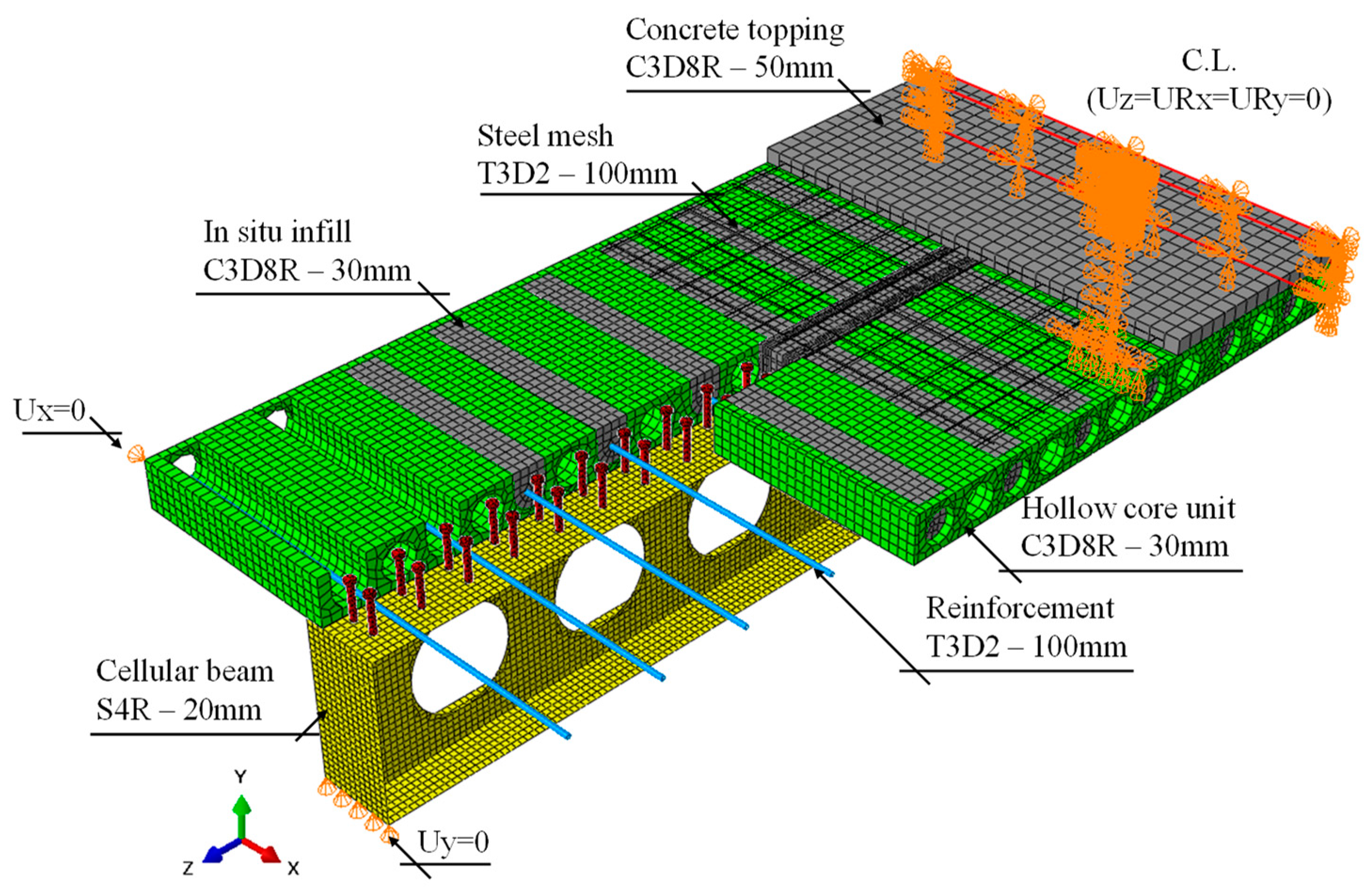
3. Finite Element Method

This section describes the methodology for developing the finite element (FE) models. This task is thoroughly detailed in previous studies by Ferreira et al. [12,22]. These studies include tables and figures that illustrate the geometric and physical characteristics of each test considered in this validation study. The FE model is based on four tests of simply supported composite cellular beams [23,24] and three tests of simply supported composite beams with PCHCS [25,26]. Geometric and material nonlinear analyses are conducted in the ABAQUS^® [27] software (version 6.24). The concrete is modelled via concrete damage plasticity (CDP) [28,29,30] using the Carreira and Chu model [31,32]. Three constitutive models of steel are employed. The elastic-perfectly plastic model is adopted for transverse bars and steel mesh. The bilinear model with hardening is used to model the headed shear studs [33]. A multilinear model, proposed by Yun and Gardner [34], is used to model the steel profiles. The interactions between steel and concrete are made using tangential and normal behaviours [35]. Regarding the discretization, S4R, C3D8R and T3D2 elements are used. The size of the finite element mesh is based on previous studies [36,37].

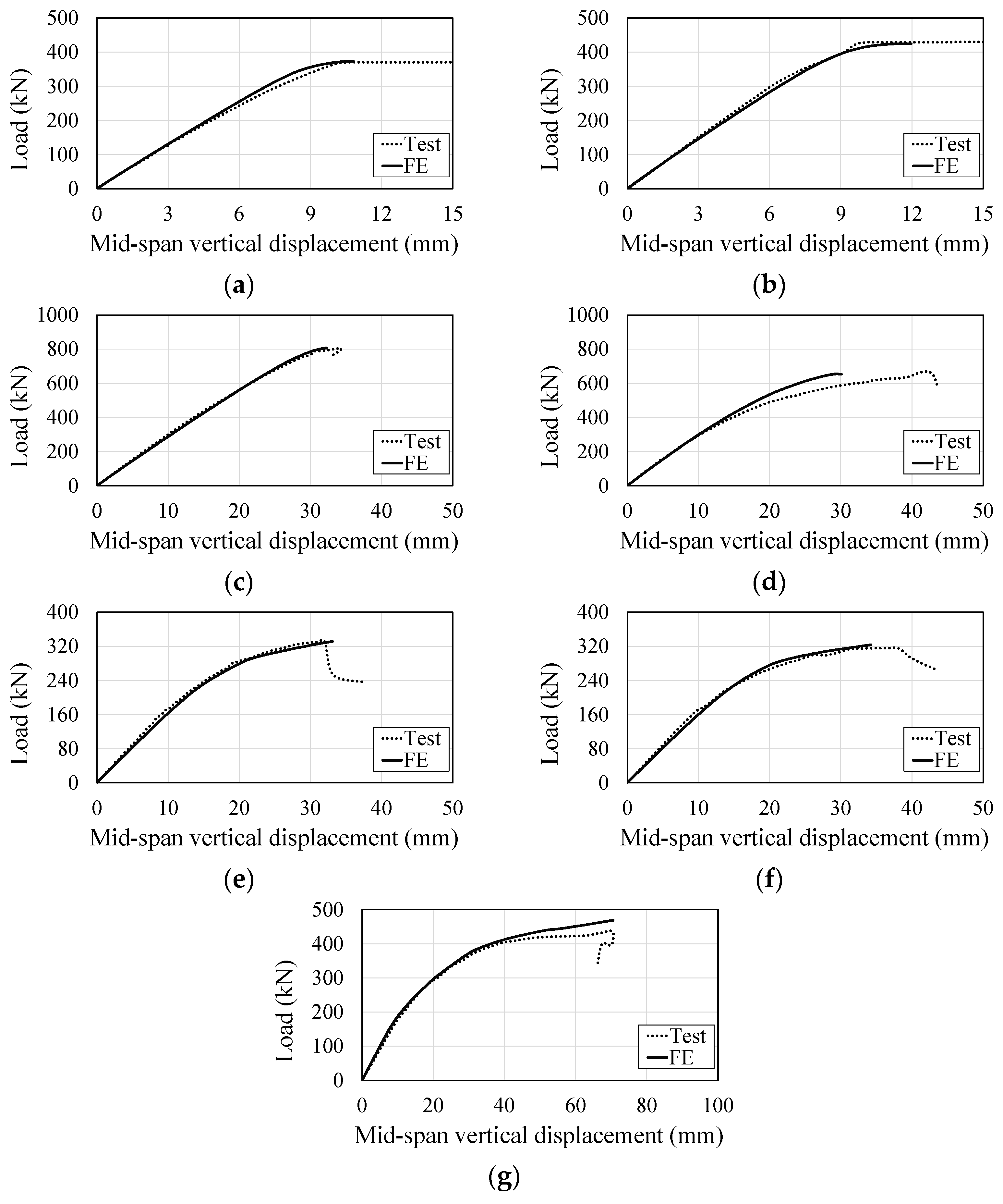
3.1. Validation Results

Figure 1 shows the validation results by load per displacement relationships. Models 1–4 and 5–7 refer to composite cellular beams and composite beams with PCHCS, respectively. Models 1–4 failed due to web-post bucking, while models 5–7 failed due to excessive cracking of the precast hollow-core slabs and steel yielding. According to all the results, it can be stated that the finite elements are validated. Further details on the results of the validation study, along with comparative analyses of the deformed configurations between the tests and the finite elements (FEs), can be found in Ferreira et al. [12,22].

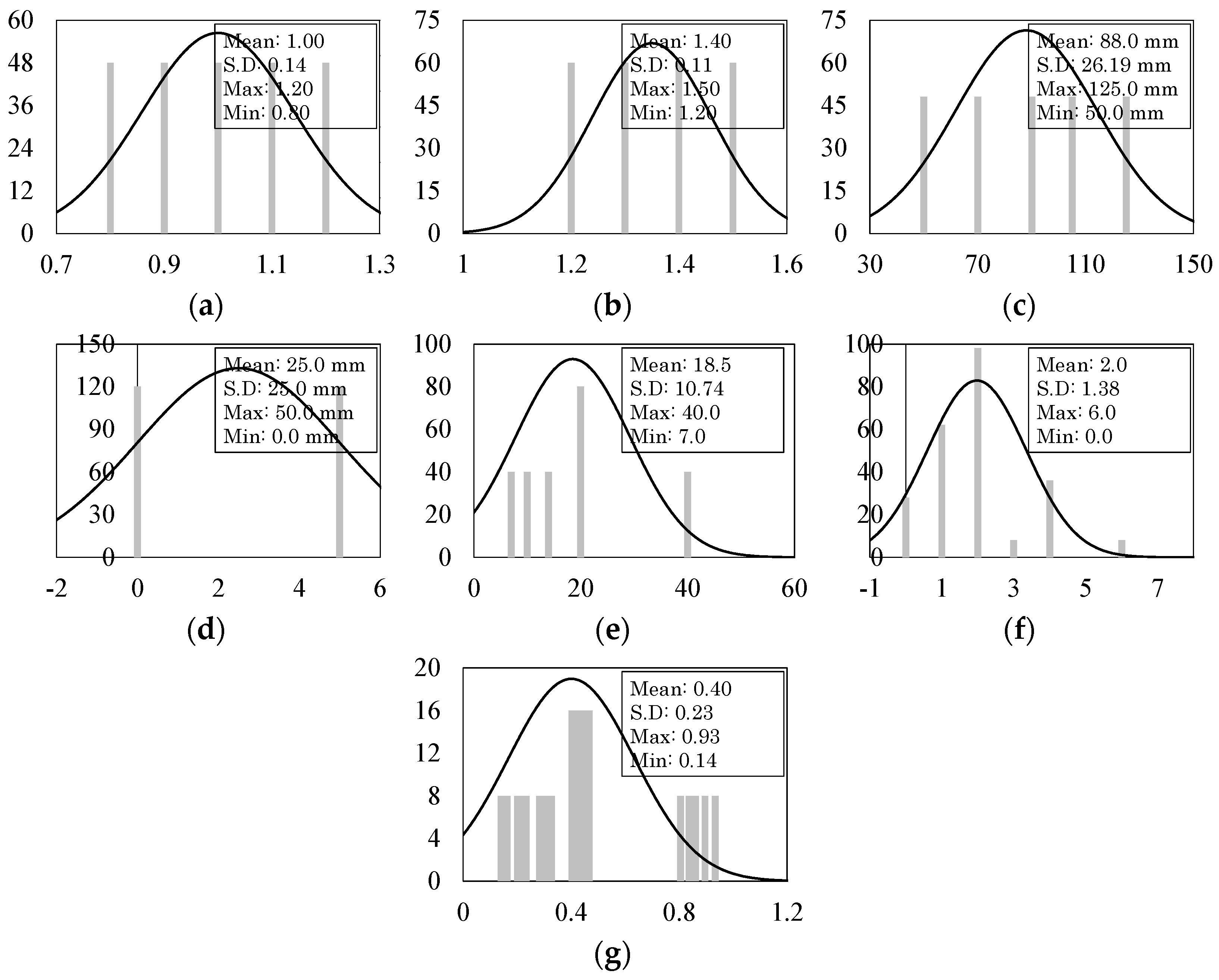
3.2. Parametric Study

In total, 240 finite element models were developed as shown in Figure 2, in which D_o is the opening diameter, d is the depth of the parent section, p is the length between the opening diameter centres, h_t is the height of the tee section, t_c is the height of the concrete topping, n is the number of shear studs between zero and the maximum moment regions, n_h is the number of shear studs above the web opening, and η is the interaction degree. The number of models considered in the parametric analyses is presented in Figure 3.

4. Machine Learning Models

When it comes to analysing a dataset, various methods can be employed to extract valuable insights. This research compares different methods to examine their effectiveness in analysing the same dataset. By examining each approach, the most suitable method will be found. In the following sections, the different methods and their applicability are explored.

4.1. CatBoost

Prokhorenkova et al. [38] recently inherited CatBoost, a gradient-boosting algorithm. A multi-platform gradient boosting library known as CatBoost solves both regression and classification problems simultaneously. Gradient boosting is successively fitted to the decision tree in the CatBoost algorithm, which uses the decision tree as the underlying weak learner. Gradient learning information is arranged inconsistently to avoid overfitting when implementing the CatBoost algorithm [39]. Figure 4 shows an explanation of the CatBoost algorithm. The CatBoost algorithm’s training ability is determined by its framework hyperparameters, such as the number of iterations, learning rate, maximum depth, etc. A model’s hyperparameters can be determined by the user and it is a laborious process.

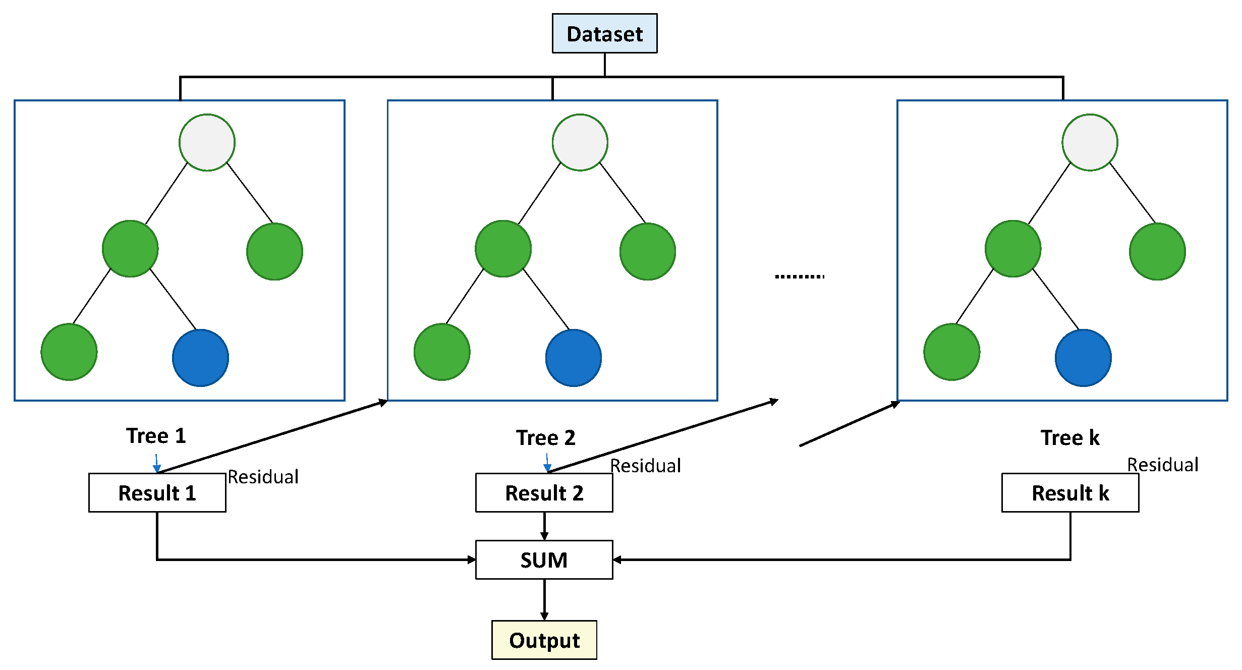
4.2. Gradient Boosting

A gradient boosting decision tree (GBDT) is a supervised machine learning model that learns a function mapping from known input variables to target variables through an algorithm. It has been deployed as the fundamental component of the embedded failure prediction methodology due to its capability to handle complex relationships and interaction effects between measured inputs automatically [40]. It provides better interpretability than other machine learning approaches like support vector machines or neural networks [41], and lower computational complexity, which makes it realistic to utilise and implement to produce valuable prediction results in a real world production environment [42,43,44]. As illustrated in Figure 5, the GBDT consists of a series of decision trees with each successive one correcting the error of the precedent trees.

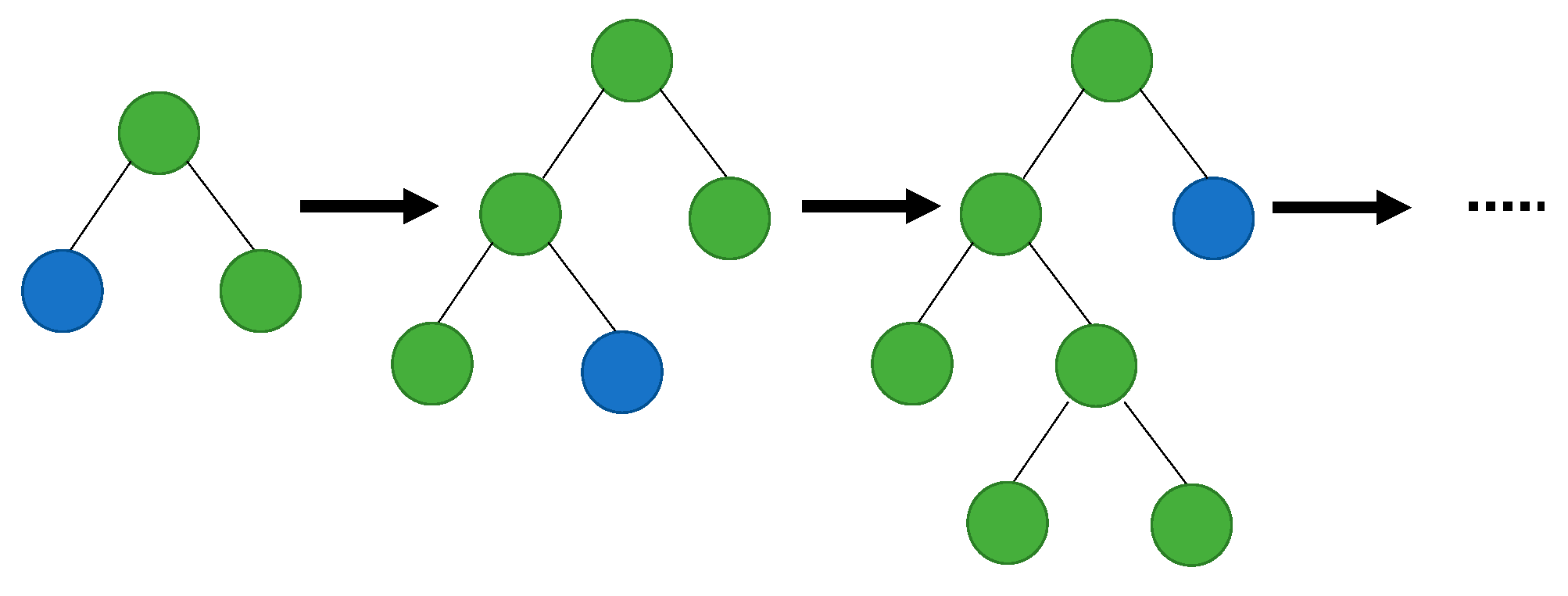
4.3. Extreme Gradient Boosting

Extreme gradient boosting (XGBoost) is an important ensemble learning algorithm in machine learning approaches [45]. In XGBoost, regression and classification trees are combined with analytical boosting methods. As an alternative to developing an addressed tree, the boosting method constructs different trees and then connects them to estimate a systematic predictive algorithm. Gradient boosting algorithms are usually matched to XGBoost’s subsequent assessment of the loss function. There are many ways to mine the characteristics of gene coupling using XGBoost. The general structure of XGBoost models is shown in Figure 6.

4.4. Light Gradient Boosting Machine

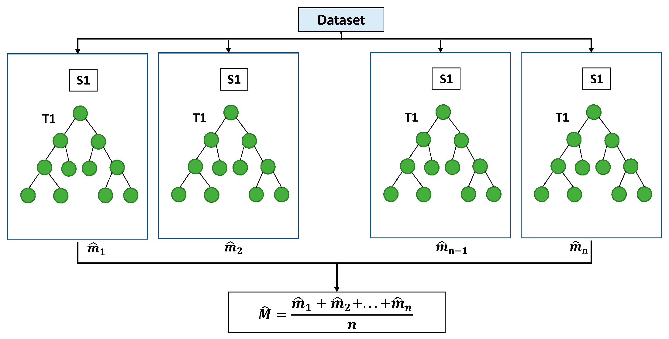
The light gradient boosting machine, or LightGBM, is an open source graded boosting machine learning model from Microsoft based on decision trees [47]. With LightGBM, continuous buckets of elemental values are divided into separate bins with greater adeptness and a faster training rate. With histogram-based algorithms, the learning phase is improved, memory consumption is reduced, and communication networks are integrated to enhance training regularity, known as parallel voting decision trees. To select the top-k elements and apply global voting techniques, the data to be learned are partitioned into several trees. Figure 7 illustrates how LightGBM identifies the leaf with the maximum splitter gain using a leaf-wise approach [48].

4.5. Random Forest

A random forest combines multiple decision trees to reduce overfitting and bias-related inaccuracy, resulting in usable results. It is a powerful and versatile algorithm that grows and combines multiple decision trees to create a “forest” [49]. It can handle large data sets due to its capability to work with many variables, running into the thousands [50]. The RF model’s basic structure is shown in Figure 8.

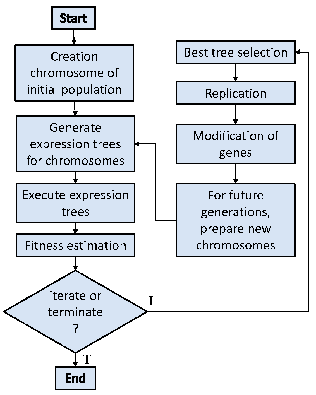
4.6. Gene Expression Programming

Genetic algorithms (GAs) were pioneered by J. Holland [52], drawing inspiration from Darwin’s theory of evolution. GAs mirror the biological evolution process, representing solutions through fixed chromosomes. Similarly, genetic programming (GP) was introduced by Cramer and advanced by Koza [53,54]. GP extends GAs, functioning as a form of machine learning that constructs models via genetic evaluation. Operating on Darwinian reproduction principles, GP stands as a powerful optimization technique leveraging neural networks and regression methods. Further, Ferreira [55] proposed a modified version of GP based on population evolution, dubbed gene expression programming (GEP). GEP encodes chromosomes in a linear fixed array, outperforming GP, which uses a tree-like structure with variable lengths [56]. A linear fixed length chromosome and a nonlinear expression tree were inherited from GAs and GP in the evolutionary GEP algorithm, respectively. The linear fixed width of genetic programming and the genetic algorithm make GEP an excellent method. Figure 9 [57] shows a schematic diagram of the GEP algorithm. Based on the experimental results, GEP itself adds and deletes various parameters.

5. Assessing the Accuracy of Machine Learning Models

To assess how accurately a machine learning model can make predictions, its accuracy needs to be measured. Some of the metrics that are often used to measure the performance of regression models are the mean squared error (MSE), the mean absolute error (MAE), the root mean squared error (RMSE), the coefficient of determination (R²), the mean absolute percentage error (MAPE) and the root mean squared logarithmic error (RMSLE) [58,59,60,61], according to Equations (1)–(6).

$$\mathrm{M}\mathrm{S}\mathrm{E}={\displaystyle \frac{1}{n}}\sum _{i=1}^n {(y_i-{\widehat{y}}_i)}^2$$

(1)

$$\mathrm{M}\mathrm{A}\mathrm{E}={\displaystyle \frac{1}{n}}\sum _{i=1}^n‍|y_i-{\widehat{y}}_i|$$

(2)

$$\mathrm{R}\mathrm{M}\mathrm{S}\mathrm{E}=\sqrt{{\displaystyle \frac{{\sum }_{i=1}^n{(y_i-{\widehat{y}}_i)}^2}{n}}}$$

(3)

$${\mathrm{R}}^2=1-{\displaystyle \frac{{\sum }_{i=1}^n‍{(y_i-{\widehat{y}}_i)}^2}{\sum ‍i=1^n{(y_i-\overline{y})}^2}}$$

(4)

$$\mathrm{M}\mathrm{A}\mathrm{P}\mathrm{E}={\displaystyle \frac{100}{n}}\sum _{i=1}^n‍\left|{\displaystyle \frac{y_i-{\widehat{y}}_i}{y_i}}\right|$$

(5)

$$\mathrm{R}\mathrm{M}\mathrm{S}\mathrm{L}\mathrm{E}=\sqrt{{\displaystyle \frac{1}{n}}\sum _{i=1}^n‍{\left[\mathrm{l}\mathrm{o}\mathrm{g}(1+y_i)-\mathrm{l}\mathrm{o}\mathrm{g}(1+{\widehat{y}}_i)\right]}^2}$$

(6)

Here, $n$ is the total number of observations, $y_i$ is the actual value, ${\widehat{y}}_i$ is the predicted value, and $\overline{y}$ is the mean of the actual value.

6. Results and Discussion

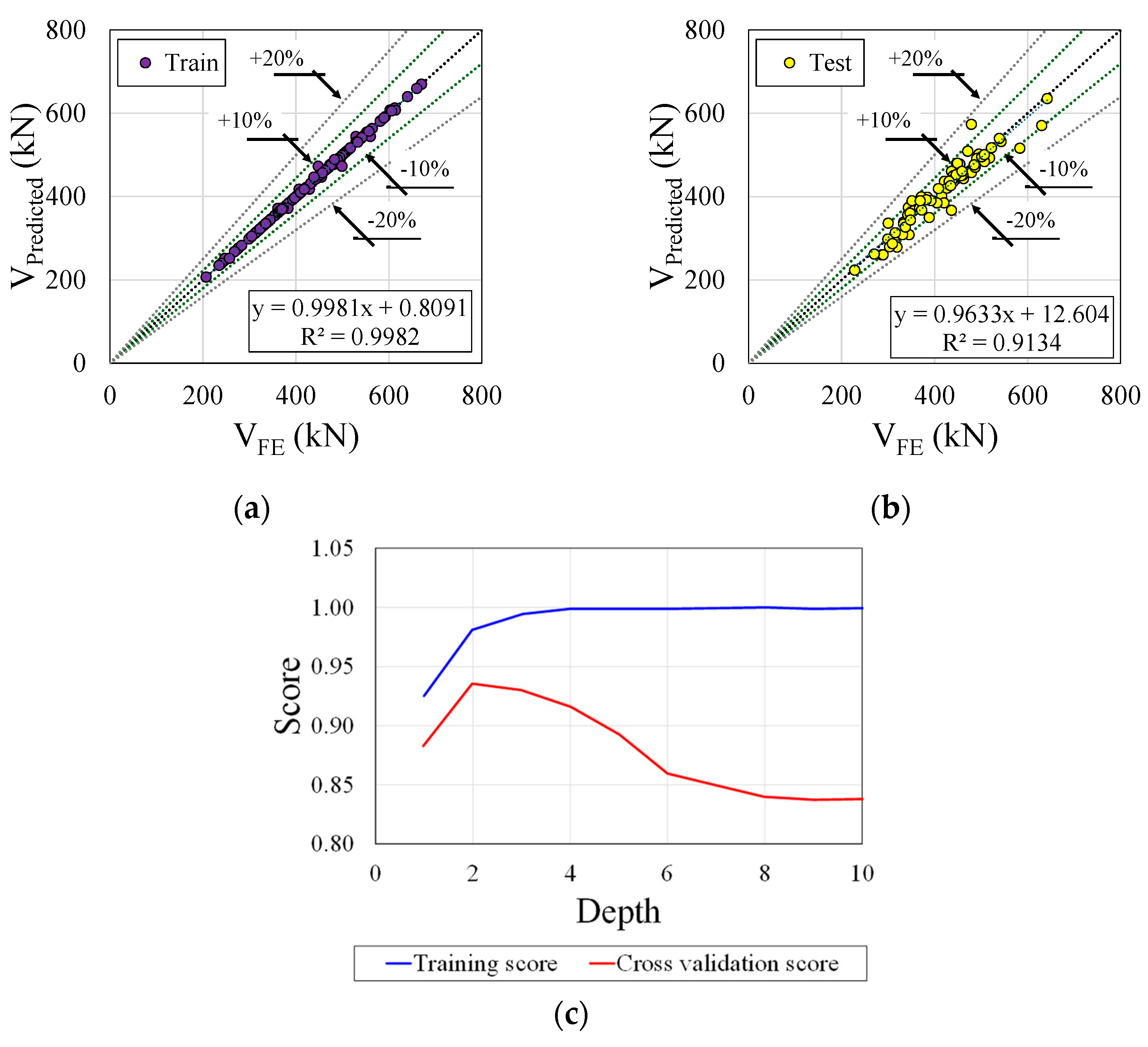
In this section, the performance of each algorithm used to predict the shear capacity of four composite cellular beams with PCHCS will be discussed.

Table 1. Model hyperparameters.

Description	Value
Session ID	1991
Original data shape	(240, 11)
Transformed train set shape	(168, 11)
Transformed test set shape	(72, 11)
Categorical imputation	mode
Normalize method	robust
Fold generator	KFold
Fold number	10
Transform target method	yeo-johnson

provides details of the hyperparameters related to the models.

6.1. CatBoost

Figure 10a,b show the train and test plots, respectively, and the validation curve (Figure 10c) of the CatBoost regressor. According to the illustration, the residual distribution around zero is highly concentrated, indicating excellent model precision. Its robust performance is underscored by its high train R² value of 0.997 and test R² value of 0.939, which indicates that the CatBoost regressor model is both highly precise and highly generalizable. Regarding the validation curve, with a depth of 0, the training score starts at approximately 1.0, which indicates that the model is able to fit the training data well with a shallow tree. With increasing depth, the training score decreases slightly, suggesting that the model is becoming less prone to overfitting and more generalised. Initially, the cross-validation score is lower than the training score, but it peaks around 4 when the depth increases. It is evident from this validation curve that the model is performing well; however, beyond the depth of 4, there is a noticeable divergence between the training and validation scores. The model performs exceptionally well on trained data, but less so on unseen or validation data as a result of mild overfitting.

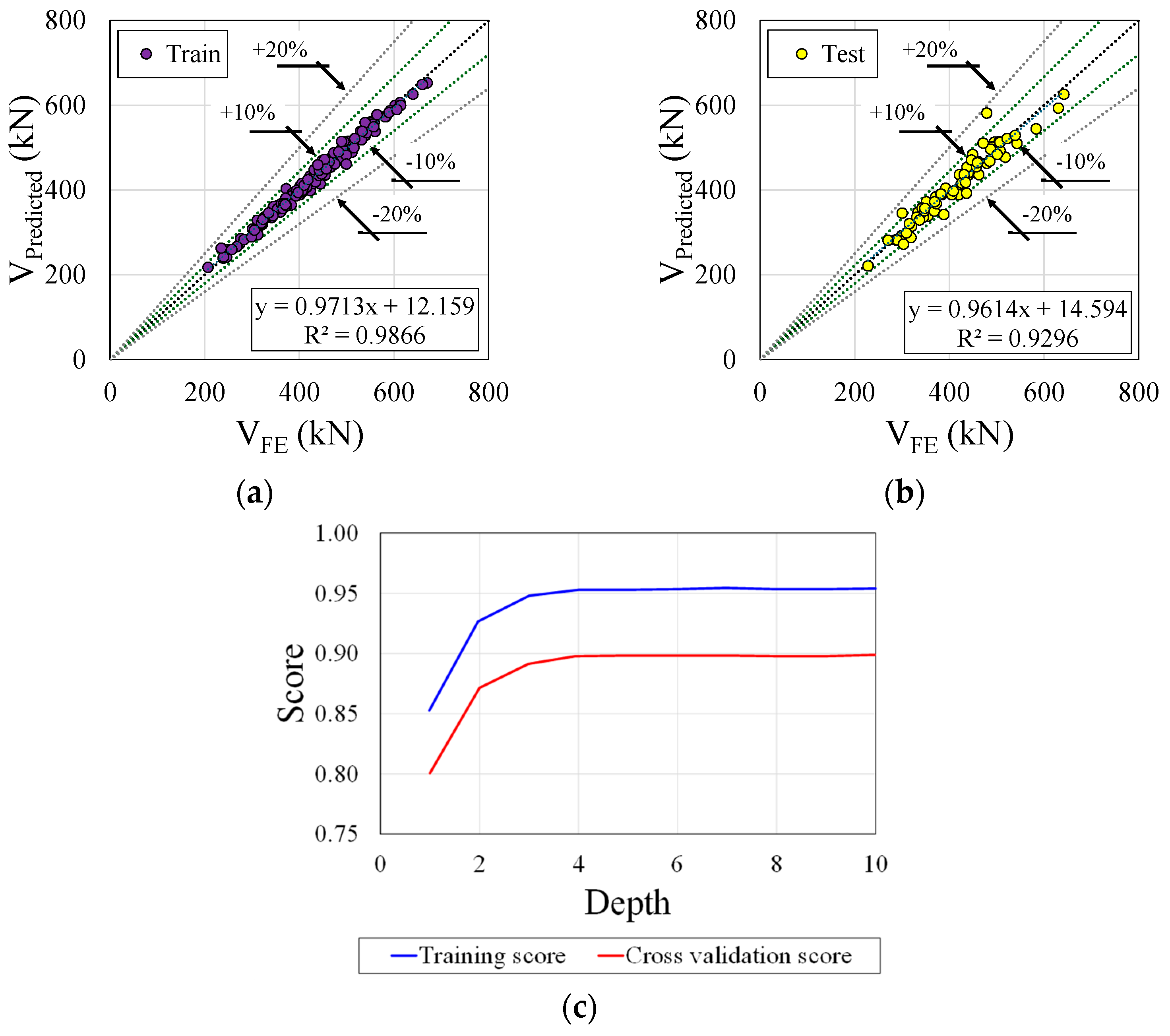
6.2. Gradient Boosting

A regression model typically assumes that the residuals are approximately normally distributed around zero based on the histogram on the right side of the plot (Figure 11). The absence of clear outliers in the residuals is a positive sign, as outliers can significantly affect model fitting. As a result of the model explaining a large proportion of the variance in the dependent variable, the R-squared values for both the train and test sets are quite high (0.9557 and 0.9118, respectively). It is possible to have an overfitted model despite having a high R-squared. It can be seen from Figure 11c that the model exhibits strong learning and generalization capabilities. As the model complexity (depth) increases, the risk of overfitting increases too. In order to achieve a balance between the bias and variance, the optimal model depth appears to be around 6, when the cross-validation score is maximised.

6.3. Extreme Gradient Boosting

The residual plot is similar to that for CatBoost (Figure 12a), but with slightly more dispersion, as indicated by its similar R² values for train (0.9982) and test (0.9134), respectively. Even though the XGB regressor model is highly precise on the training data, it may not generalize as well to unseen data. Regarding the validation curve, as shown in Figure 12, as the depth increases, the cross-validation score (noted by the green line with circular markers) begins lower than the training score but grows as the depth increases, reaching a peak at around 4. These scores are shaded to illustrate their variance or uncertainty. This validation curve is indicative of a well-performing model; however, a noticeable divergence exists between the training and validation scores beyond the depth of 4. Essentially, this divergence indicates a mild overfitting scenario in which the model performs exceptionally well on the trained data, but less so on unseen or validation data.

6.4. Light Gradient Boosting Machine

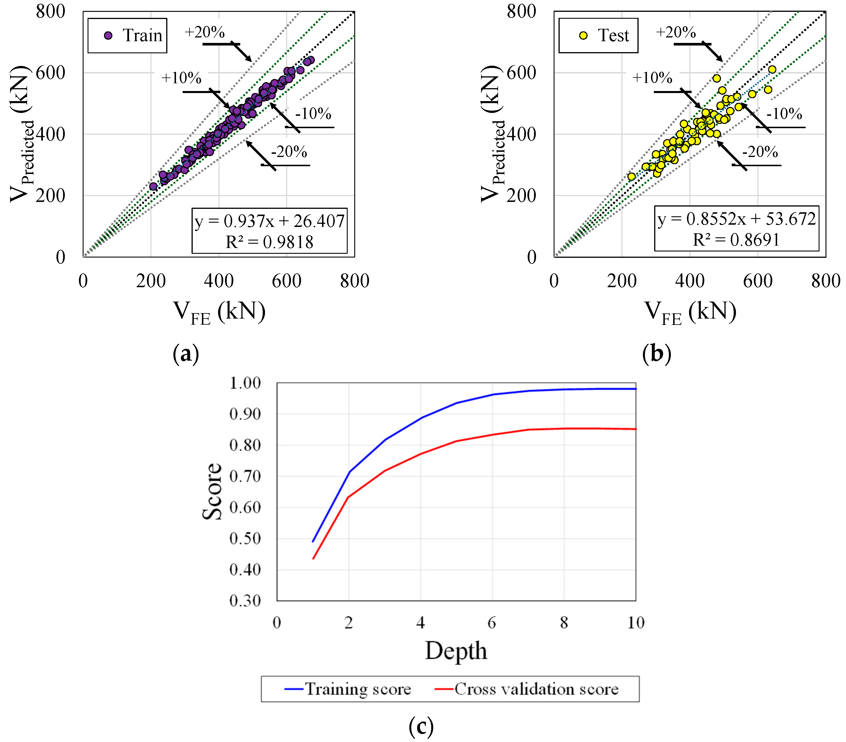
Figure 13 shows the residual plot (Figure 13a) and validation curve (Figure 13b) for the light gradient boosting machine model. This model has a dispersed residual distribution with significant variance at higher predicted values. Despite having a high train R² value (0.9866), the test R² is significantly lower 0.9296, suggesting possible overfitting. Consequently, although the light GBM regressor performs well on the training data, it may not generalize to unknown data. Considering the validation curve with a depth of 2, the training score starts at a high score of approximately 0.95, which implies that the model is able to fit the training data quite well with a shallow tree. As the depth increases, the training score decreases slightly, suggesting that the model is becoming more generalised and less likely to overfit. In contrast to the training score, the cross-validation score exhibits an upward trend as the depth increases, reaching a peak of around 4. There is a noticeable divergence between the training and validation scores beyond the depth of 4, which indicates that the model performs exceptionally well on the trained data, but significantly less well on unseen or validation data. This divergence indicates mild overfitting.

6.5. Random Forest

Figure 14 shows the performance of the random forest model. This model presents an intermediate residual spread with some concentration around zero but noticeable dispersion at the extremes (Figure 14a). As a result, the random forest regressor model appears to offer a good balance between precision and generalization, but there is room for further optimization. A train R² of 0.980 and test R² of 0.871 suggest moderate model accuracy, though room for improvement exists. For the validation curve (Figure 14b) at a depth of around 6, the cross-validation score reaches a peak, indicating the variance and uncertainty associated with the scores. The shaded area around this line illustrates the variance or uncertainty associated with the scores. Despite the fact that this validation curve indicates that the model is performing well, there is a noticeable divergence between the training and validation scores beyond a depth of 6. In this case, mild overfitting occurs when the model does exceptionally well on the trained data but less so on unseen or validation data.

6.6. Feature Importance

Figure 15 is a feature importance plot, which is commonly used in machine learning to understand the contribution of each parameter analysed. The y-axis in this plot represents the different features used in the model, while the x-axis represents the importance of each feature. The importance of a feature is calculated based on the decrease in the model’s performance when the feature’s values are randomly shuffled. The highest importance value in the plot is associated with the p/D_o feature, suggesting that it has the most significant impact on the model’s predictions. Changes in this feature are likely to result in significant changes in the predicted output. The η and n features also have high importance values and significantly influence model predictions. Although other features have lower importance values, they can still be useful in interactions with other features. Therefore, it is essential to consider all features when building a machine learning model, as even low importance features can have an impact on the overall performance of the model. Understanding feature importance can help data scientists optimize machine learning models and improve their accuracy.

7. Proposed Equation by GEP

To precisely predict the shear capacity of composite cellular floors with PCHCS, this study developed an equation incorporating all relevant parameters. These parameters included mechanical and geometric properties, as well as the areas and detailing of reinforcements within the joint. Numerical constants are critical for successful modelling in GEP’s learning algorithms. Thus, GEP employs an extra gene domain to encode these random constants. Initially, these constants are randomly assigned to each gene. However, the standard genetic operators of mutation (including transposition and recombination) ensure their continued circulation and diversity throughout the population. The specific details regarding the proposed model’s operation and functionality are outlined in

Table 2. Model construction parameters.

Function Set	+, −, *, /, Exp, Ln
Number of generations	365,000
Chromosomes	200
Head size	14
Linking function	Addition
Number of genes	3
Mutation rate	0.044
Inversion rate	0.1
One-point recombination rate	0.3
Two-point recombination rate	0.3
Gene recombination rate	0.1
Gene transposition rate	0.1
Constants per gene	2
Lower/upper bound of constants	−10/10

.

Several preliminary runs were necessary to identify the parameter settings that produce a GEP model with sufficient robustness and generalization to accurately solve the problem. Additionally, overfitting, a common issue in machine learning, constitutes another challenge to achieving satisfactory generalization. To avoid this issue, the developed models can be tested. The proposed equations (Equations (7)–(12)) for predicting the shear capacity of steel–concrete composite cellular floors with precast hollow-core slabs using the GEP model are as follows, in which E is the Young’s modulus, ν is the Poisson’s ratio, f_y is the yield stress, and f_v is the yield shear stress:

$$\left(N\right)=\left\{\begin{array}{cc}{\eta }^{0.14}{\left({\displaystyle \frac{V_{cr}}{V_y}}\right)}^{-0.12}{V}_y& {\lambda }_{\mathrm{v}}\le 0.68\\ {\eta }^{0.14}\left[1-0.0026{\left({\displaystyle \frac{V_{cr}}{V_y}}\right)}^{4.7}\right]{\left({\displaystyle \frac{V_{cr}}{V_y}}\right)}^{0.04}{V}_y& {0.68<\lambda }_{\mathrm{v}}\le 1.01\\ 35250 \ln \left(V_{cr}\right)+{\eta }^{3.03} {V_{cr}}^{0.91}& {\lambda }_{\mathrm{v}}>1.01\end{array}\right.$$

(7)

$$V_{cr}={\displaystyle \frac{{\pi }^{2}E{A}_w}{12\left(1-{\upsilon }^2\right){\left(b_w/t_w\right)}^2}}$$

(8)

$$A_w=\left(d_g-D_0\right)t_w$$

(9)

$$V_y=A_w{f}_{\mathrm{v}}$$

(10)

$$f_{\mathrm{v}}=f_y/\sqrt{3}$$

(11)

$${\lambda }_{\mathrm{v}}=\sqrt{V_y/V_{cr}}$$

(12)

8. Comparison Analysis

The comparative analysis is depicted in Figure 16, encompassing all explored machine learning models. The discussion revolves around the ratio of predicted values to the finite element model (V_Predicted/V_FE). Focusing on the CatBoost algorithm (Figure 16a), the range of relative errors extends from −13.90% to 16.54%. Meanwhile, the gradient boosting algorithm (Figure 16b) exhibits relative errors ranging from −11.76% to 21.41%. In the case of the extreme gradient algorithm (Figure 16c), the spectrum of relative errors spans from −18.12% to 22.99%. As for the light gradient boosting algorithm (Figure 16d), its minimum and maximum relative errors align closely with the gradient boosting algorithm, standing at −11.77% and 24.00%, respectively. Turning to the random forest algorithm (Figure 16e), the relative errors fluctuate between −16.50% and 21.48%. Lastly, gene expression programming (Figure 16f) provides relative errors ranging from −12.84% to 2.69%. Additional summarized statistical analyses are presented in

Table 3. Machine learning models comparative analysis.

Analysis	Catboost	Gradient Boosting	Extreme Gradient	Light Gradient Boosting	Random Forest	GEP
R2	0.9821	0.9694	0.9762	0.9442	0.9186	0.9531
RMSE (kN)	12.1504	15.3435	16.5446	21.5878	20.3665	30.1683
MAE (kN)	6.7814	10.9457	7.4057	16.5853	14.1428	24.8799
Minimum relative error	−13.90%	−11.76%	−18.12%	−11.77%	−16.50%	−12.84%
Maximum relative error	16.54%	21.41%	22.99%	24.00%	21.48%	2.69%
Mean	1.000	1.000	1.000	1.000	0.998	0.945
SD	2.86%	3.66%	3.88%	5.28%	4.79%	4.51%
CoV	2.86%	3.66%	3.88%	5.28%	4.80%	4.77%

.

9. Reliability Analysis

Reliability analysis based on Annex D EN 1990 (2002) [62] has been conducted to assess the proposed design method and propose a partial safety factor for the shear capacity of composite cellular beams with PCHCS. Within the context of this study, the proposed prediction models underwent statistical evaluation against the finite element results.

Table 4. Summary of the reliability analysis calculated according to EN 1990.

Machine Learning Model	n	$\overline{\mathit{b}}$	${\mathit{k}}_{\mathit{d},\mathit{n}}$	${\mathit{k}}_{\mathit{n}}$	Vr	${\mathit{\gamma }}_{\mathit{M}0}$
Catboost	240	1.00	3.04	1.64	0.163	1.255
Gradient boosting	240	1.002	3.04	1.64	0.163	1.257
Extreme gradient	240	0.999	3.04	1.64	0.163	1.258
Light gradient boosting	240	1.004	3.04	1.64	0.161	1.265
Random forest	240	1.009	3.04	1.64	0.165	1.263
GEP	240	1.058	3.04	1.64	0.161	1.263

illustrates the key statistical parameters, including the amount of data, $n$, the design fractile factor (ultimate limit state), $k_{d,n}$, the characteristic fractile factor, $k_n$, the average ratio of FE to resistance model predictions based on the least squares fit to the data, $\overline{b}$, the combined coefficient of variation incorporating both resistance model and basic variable uncertainties, $V_r$, and the partial safety factor for resistance, ${\gamma }_{M0}$. The COV for geometric dimensions of the concrete slab is 0.04 for the width and the thickness [63], while it is 0.02 for the steel section geometries [64] and the stud diameter [65].

The COV (V_x) of the yield strength of steel, ultimate strength of the steel stud, and concrete compressive strength were assumed equal to 0.055 [64], 0.05 and 0.12 [65], respectively. The COV between the experimental and the numerical results, which were found equal to 0.025, was also considered. Performing the first order reliability method (FORM) in accordance with the Eurocode target reliability requirements, the partial factors ${\gamma }_{M0}$ were evaluated for all ML models using the following procedure.

First, we estimate the mean value correction factor b:

$$b={\displaystyle \frac{\sum r_e{r}_t}{\sum r_t^2}}$$

(13)

Here, r_e and r_t are the experimental and theoretical resistance, respectively.

The error term δ_i for each experimental value r_ei should be determined from:

$${\delta }_i={\displaystyle \frac{r_{ei}}{b{r}_{ti}}}$$

(14)

The coefficient of variation for the error term δ_i can be estimated from:

$$V_{\delta }=\sqrt{\exp \left(s_{∆}^2\right)-1}$$

(15)

where:

$$s_{∆}={\displaystyle \frac{1}{n-1}}\sum _{i=1}^n{\left({∆}_i-\overline{∆}\right)}^2$$

(16)

The estimated value of $\overline{∆}$ is taken as:

$$\overline{∆}={\displaystyle \frac{1}{n}}\sum _{i=1}^n{∆}_i$$

(17)

${∆}_i$ is the logarithm of the error term ${\delta }_i$:

$${∆}_i=\mathrm{l}\mathrm{n}\left({\delta }_i\right)$$

(18)

The coefficient of variation V_r can be determined from:

$$V_r^2=\left(V_{\delta }^2+1\right)\left[\prod _{i=1}^j\left(V_{Xi}^2+1\right)\right]-1$$

(19)

with:

$$V_{rt}^2=\sum _i^j{V}_{Xi}^2$$

(20)

V_xi is the coefficient of variation for the yield strength of the steel, the ultimate strength of the steel stud, the concrete compressive strength, and the coefficient of variation between the experimental and the numerical results. It is also for the geometric dimensions of the concrete slab, the steel section, and the stud diameter.

The characteristic resistance r_k is obtained from:

$$r_k=b{g}_{rt}\left(\underset{\_}{X_m}\right)\exp \left(-k_{\mathrm{\infty }}{\alpha }_{rt}{Q}_{rt}-k_{\mathrm{n}}{\alpha }_{\delta }{Q}_{\delta }-0.5Q^2\right)$$

(21)

with:

$$\begin{gathered} Q_{rt}=\sqrt{ln\left(V_{rt}^2+1\right)} \\ {Q}_{\delta }=\sqrt{ln\left(V_{\delta }^2+1\right)} \\ Q=\sqrt{ln\left(V_r^2+1\right)} \\ {\alpha }_{rt}={\displaystyle \frac{Q_{rt}}{Q}} \\ {\alpha }_{\delta }={\displaystyle \frac{Q_{\delta }}{Q}} \end{gathered}$$

(22)

The notation is as follows:

k_n is the characteristic fractile factor from table D 1 for the unknown case V_x;

$k_{\mathrm{\infty }}$ is the value of k_n for $n\to \mathrm{\infty }[k_{\mathrm{\infty }}=1.64]$;

${\alpha }_{rt}$ is the weighting factor for $Q_{rt}$;

${\alpha }_{\delta }$ is the weighting factor for $Q_{\delta }$.

The design value r_d is obtained from:

$$r_d=b{g}_{rt}\left(\underset{\_}{X_m}\right)\exp \left(-k_{\mathrm{d},\mathrm{\infty }}{\alpha }_{rt}{Q}_{rt}-k_{\mathrm{d},\mathrm{n}}{\alpha }_{\delta }{Q}_{\delta }-0.5Q^2\right)$$

(23)

k_d,n is the characteristic fractile factor from table D 2 for the case V_x unknown;

$k_{\mathrm{d},\mathrm{\infty }}$ is the value of k_d,n for $n\to \mathrm{\infty }[k_{\mathrm{\infty }}=3.04]$.

The partial factor ${\gamma }_{M0}$ is:

$${\gamma }_{M0}={\displaystyle \frac{r_k}{r_d}}$$

(24)

As can be seen from Table 3, the partial factors for the shear capacity of steel–concrete composite cellular beams with precast hollow-core slabs using different ML algorithms are very similar, and the values are around 1.255 to 1.265. It is worth noting that the high value for the partial factor is due to the high value for the COV of the concrete strength.

10. Conclusions

The present work aimed to apply machine learning models for predicting the global shear capacity of composite cellular floors with PCHCS. The motivation for this was the connection between the hollow-core unit and the steel cellular beam, as the deflections are intensified due to the web openings, causing the effect of pulling out the shear connector and thus reducing the local composite action. This first study, considering the application of machine learning to predict the global shear resistance of steel–concrete composite cellular beams with hollow-core units, highlights the importance of the degree of interaction in the resistance of the local composite action. A finite element model database, considering steel–concrete composite cellular beams with precast hollow-core units, was employed to assess the CatBoost, gradient boosting, extreme gradient boosting, light gradient boosting machine, random forest and gene expression programming algorithms, since there are no calculation recommendations for these beams. It was concluded that:

i.

The CatBoost regressor produced an MAE of 6.7814 kN and demonstrated commendable performance with a R² value of 0.9821, explaining around 98.21% of the variance. This study highlighted the effectiveness of the CatBoost regressor due to its low MAE and high R² value, providing valuable insights for the design and assessment of steel–concrete composite cellular beams.

ii.

With a coefficient of determination (R²) of 0.9531, the gene expression programming model displayed exceptional ability. This indicates that the model predicted approximately 95.31% of the variance in the shear capacity, establishing a strong correlation between predictions and actual values. With its promising results, gene expression programming emerges as a promising alternative for further research.

iii.

A GEP-based equation was proposed to predict the global shear of composite cellular beams with PCHCS. The suggested equation for predicting the global shear resistance highlights areas necessitating revisions and offers insights into how these improvements can be achieved. It can contribute to both the safety and cost-effectiveness of steel–concrete composite construction, especially regarding sustainability.

iv.

A reliability analysis was performed and the partial safety factor for resistance varied between 1.25 and 1.26.

References

1. Lawson, R.M.; Lim, J.; Hicks, S.J.J.; Simms, W.I.I. Design of Composite Asymmetric Cellular Beams and Beams with Large Web Openings. J. Constr. Steel Res. 2006, 62, 614–629. [Google Scholar] [CrossRef]
2. Lawson, R.M.; Saverirajan, A.H.A. Simplified Elasto-Plastic Analysis of Composite Beams and Cellular Beams to Eurocode 4. J. Constr. Steel Res. 2011, 67, 1426–1434. [Google Scholar] [CrossRef]
3. Ahmed, I.M.; Tsavdaridis, K.D. The Evolution of Composite Flooring Systems: Applications, Testing, Modelling and Eurocode Design Approaches. J. Constr. Steel Res. 2019, 155, 286–300. [Google Scholar] [CrossRef]
4. Pajari, M.; Koukkari, H. Shear Resistance of PHC Slabs Supported on Beams. I: Tests. J. Struct. Eng. 1998, 124, 1050–1061. [Google Scholar] [CrossRef]
5. Lawson, R.M.; Hicks, S.J. Design of Composite Beams with Large Web Openings. SCI P355; The Steel Construction Institute: Berkshire, UK, 2011; ISBN 9781859421970. [Google Scholar]
6. Lawson, R.M.; Lim, J.B.P.; Popo-Ola, S.O. Pull-out Forces in Shear Connectors in Composite Beams with Large Web Openings. J. Constr. Steel Res. 2013, 87, 48–59. [Google Scholar] [CrossRef]
7. Avci-Karatas, C. Application of Machine Learning in Prediction of Shear Capacity of Headed Steel Studs in Steel–Concrete Composite Structures. Int. J. Steel Struct. 2022, 22, 539–556. [Google Scholar] [CrossRef]
8. Zhang, F.; Wang, C.; Zou, X.; Wei, Y.; Chen, D.; Wang, Q.; Wang, L. Prediction of the Shear Resistance of Headed Studs Embedded in Precast Steel–Concrete Structures Based on an Interpretable Machine Learning Method. Buildings 2023, 13, 496. [Google Scholar] [CrossRef]
9. Momani, Y.; Tarawneh, A.; Alawadi, R.; Momani, Z. Shear Strength Prediction of Steel Fiber-Reinforced Concrete Beams without Stirrups. Innov. Infrastruct. Solut. 2022, 7, 107. [Google Scholar] [CrossRef]
10. Hosseinpour, M.; Rossi, A.; Sander Clemente de Souza, A.; Sharifi, Y. New Predictive Equations for LDB Strength Assessment of Steel–Concrete Composite Beams. Eng. Struct. 2022, 258, 114121. [Google Scholar] [CrossRef]
11. Thai, H.-T. Machine Learning for Structural Engineering: A State-of-the-Art Review. Structures 2022, 38, 448–491. [Google Scholar] [CrossRef]
12. Ferreira, F.P.V.; Tsavdaridis, K.D.; Martins, C.H.; De Nardin, S. Composite Action on Web-Post Buckling Shear Resistance of Composite Cellular Beams with PCHCS and PCHCSCT. Eng. Struct. 2021, 246, 113065. [Google Scholar] [CrossRef]
13. Fares, S.S.; Coulson, J.; Dinehart, D.W. AISC Steel Design Guide 31: Castellated and Cellular Beam Design; American Institute of Steel Construction: Chicago, IL, USA, 2016. [Google Scholar]
14. Redwood, R.G.; Poumbouras, G. Tests of Composite Beams with Web Holes. Can. J. Civ. Eng. 1983, 10, 713–721. [Google Scholar] [CrossRef]
15. Redwood, R.G.; Poumbouras, G. Analysis of Composite Beams with Web Openings. J. Struct. Eng. 1984, 110, 1949–1958. [Google Scholar] [CrossRef]
16. Donahey, R.C.; Darwin, D. Web Openings in Composite Beams with Ribbed Slabs. J. Struct. Eng. 1988, 114, 518–534. [Google Scholar] [CrossRef]
17. Cho, S.H.; Redwood, R.G. Slab Behavior in Composite Beams at Openings. I: Analysis. J. Struct. Eng. 1992, 118, 2287–2303. [Google Scholar] [CrossRef]
18. Cho, S.H.; Redwood, R.G. Slab Behavior in Composite Beams at Openings. II: Tests and Verification. J. Struct. Eng. 1992, 118, 2304–2322. [Google Scholar] [CrossRef]
19. Ferreira, F.P.V.; Martins, C.H.; De Nardin, S. Advances in Composite Beams with Web Openings and Composite Cellular Beams. J. Constr. Steel Res. 2020, 172, 106182. [Google Scholar] [CrossRef]
20. Hicks, S.J.; Lawson, R.M. Design of Composite Beams Using Precast Concrete Slabs. SCI P287; The Steel Construction Institute: Berkshire, UK, 2003; ISBN 1859421393. [Google Scholar]
21. Gouchman, G.H. Design of Composite Beams Using Precast Concrete Slabs in Accordance with EUROCODE 4. SCI P401; The Steel Construction Institute: Berkshire, UK, 2014; ISBN 9781859422137. [Google Scholar]
22. Ferreira, F.P.V.; Tsavdaridis, K.D.; Martins, C.H.; De Nardin, S. Ultimate Strength Prediction of Steel–Concrete Composite Cellular Beams with PCHCS. Eng. Struct. 2021, 236, 112082. [Google Scholar] [CrossRef]
23. Nadjai, A.; Vassart, O.; Ali, F.; Talamona, D.; Allam, A.; Hawes, M. Performance of Cellular Composite Floor Beams at Elevated Temperatures. Fire Saf. J. 2007, 42, 489–497. [Google Scholar] [CrossRef]
24. Müller, C.; Hechler, O.; Bureau, A.; Bitar, D.; Joyeux, D.; Cajot, L.G.; Demarco, T.; Lawson, R.M.; Hicks, S.; Devine, P.; et al. Large Web Openings for Service Integration in Composite Floors; Technical Steel Research; European Commission, Contract No 7210-PR/315; Final Report 2006. Available online: https://op.europa.eu/en/publication-detail/-/publication/a4af7d1a-b375-4aaa-855e-4e4159737fe3 (accessed on 14 May 2024).
25. El-Lobody, E.; Lam, D. Finite Element Analysis of Steel-Concrete Composite Girders. Adv. Struct. Eng. 2003, 6, 267–281. [Google Scholar] [CrossRef]
26. Batista, E.M.; Landesmann, A. Análise Experimental de Vigas Mistas de Aço e Concreto Compostas Por Lajes Alveolares e Perfis Laminados; COPPETEC, PEC-18541 2016.
27. Dassault Systèmes Simulia Abaqus 6.18 2016; Dassault Systèmes Simulia Corporation: Providence, RI, USA, 2016.
28. Hillerborg, A.; Modéer, M.; Petersson, P.-E. Analysis of Crack Formation and Crack Growth in Concrete by Means of Fracture Mechanics and Finite Elements. Cem. Concr. Res. 1976, 6, 773–781. [Google Scholar] [CrossRef]
29. Lubliner, J.; Oliver, J.; Oller, S.; Oñate, E. A Plastic-Damage Model for Concrete. Int. J. Solids Struct. 1989, 25, 299–326. [Google Scholar] [CrossRef]
30. Lee, J.; Fenves, G.L. Plastic-Damage Model for Cyclic Loading of Concrete Structures. J. Eng. Mech. 1998, 124, 892–900. [Google Scholar] [CrossRef]
31. Carreira, D.J.; Chu, K.H. Stress-Strain Relationship for Reinforced Concrete in Tension. ACI J. Proc. 1986, 83, 21–28. [Google Scholar] [CrossRef]
32. Carreira, D.J.; Chu, K.H. Stress-Strain Relationship for Plain Concrete in Compression. ACI J. Proc. 1985, 82, 797–804. [Google Scholar] [CrossRef]
33. de Lima Araújo, D.; Sales, M.W.R.; de Paulo, S.M.; de Cresce El Debs, A.L.H. Headed Steel Stud Connectors for Composite Steel Beams with Precast Hollow-Core Slabs with Structural Topping. Eng. Struct. 2016, 107, 135–150. [Google Scholar] [CrossRef]
34. Yun, X.; Gardner, L. Stress-Strain Curves for Hot-Rolled Steels. J. Constr. Steel Res. 2017, 133, 36–46. [Google Scholar] [CrossRef]
35. Guezouli, S.; Lachal, A. Numerical Analysis of Frictional Contact Effects in Push-out Tests. Eng. Struct. 2012, 40, 39–50. [Google Scholar] [CrossRef]
36. Ferreira, F.P.V.; Martins, C.H.; De Nardin, S. A Parametric Study of Steel-Concrete Composite Beams with Hollow Core Slabs and Concrete Topping. Structures 2020, 28, 276–296. [Google Scholar] [CrossRef]
37. Ferreira, F.P.V.; Martins, C.H.; De Nardin, S. Assessment of Web Post Buckling Resistance in Steel-Concrete Composite Cellular Beams. Thin-Walled Struct. 2021, 158, 106969. [Google Scholar] [CrossRef]
38. Prokhorenkova, L.; Gusev, G.; Vorobev, A.; Dorogush, A.V.; Gulin, A. CatBoost: Unbiased Boosting with Categorical Features. In Proceedings of the NIPS’18: Proceedings of the 32nd International Conference on Neural Information Processing Systems, Red Hook, NY, USA, 3–8 December 2018; pp. 6638–6648. [Google Scholar]
39. Dorogush, A.V.; Ershov, V.; Yandex, A.G. CatBoost: Gradient Boosting with Categorical Features Support. arXiv 2018, arXiv:1810.11363. [Google Scholar]
40. Elith, J.; Leathwick, J.R.; Hastie, T. A Working Guide to Boosted Regression Trees. J. Anim. Ecol. 2008, 77, 802–813. [Google Scholar] [CrossRef]
41. Guelman, L. Gradient Boosting Trees for Auto Insurance Loss Cost Modeling and Prediction. Expert. Syst. Appl. 2012, 39, 3659–3667. [Google Scholar] [CrossRef]
42. Bentéjac, C.; Csörgő, A.; Martínez-Muñoz, G. A Comparative Analysis of Gradient Boosting Algorithms. Artif. Intell. Rev. 2021, 54, 1937–1967. [Google Scholar] [CrossRef]
43. Zhang, Y.; Beudaert, X.; Argandoña, J.; Ratchev, S.; Munoa, J. A CPPS Based on GBDT for Predicting Failure Events in Milling. Int. J. Adv. Manuf. Technol. 2020, 111, 341–357. [Google Scholar] [CrossRef]
44. Si, S.; Zhang, H.; Keerthi, S.S.; Mahajan, D.; Dhillon, I.S.; Hsieh, C.-J. Gradient Boosted Decision Trees for High Dimensional Sparse Output. Proc. Mach. Learn. Res. 2017, 70, 3182–3190. [Google Scholar]
45. Meng, Q.; Ke, G.; Wang, T.; Chen, W.; Ye, Q.; Ma, Z.M.; Liu, T.Y. A Communication-Efficient Parallel Algorithm for Decision Tree. In Proceedings of the NIPS’16: Proceedings of the 30th International Conference on Neural Information Processing Systems, Red Hook, NY, USA, 5–10 December 2016; pp. 1279–1287. [Google Scholar]
46. Liu, J.J.; Liu, J.C. Permeability Predictions for Tight Sandstone Reservoir Using Explainable Machine Learning and Particle Swarm Optimization. Geofluids 2022, 2022, 263329. [Google Scholar] [CrossRef]
47. Ke, G.; Meng, Q.; Finley, T.; Wang, T.; Chen, W.; Ma, W.; Ye, Q.; Liu, T.-Y. LightGBM: A Highly Efficient Gradient Boosting Decision Tree. In Proceedings of the Advances in Neural Information Processing Systems; Guyon, I., Von Luxburg, U., Bengio, S., Wallach, H., Fergus, R., Vishwanathan, S., Garnett, R., Eds.; Curran Associates, Inc.: Long Beach, CA, USA, 2017; Volume 30. [Google Scholar]
48. Shahani, N.M.; Zheng, X.; Guo, X.; Wei, X. Machine Learning-Based Intelligent Prediction of Elastic Modulus of Rocks at Thar Coalfield. Sustainability 2022, 14, 3689. [Google Scholar] [CrossRef]
49. Chen, X.; Ishwaran, H. Random Forests for Genomic Data Analysis. Genomics 2012, 99, 323–329. [Google Scholar] [CrossRef]
50. Schonlau, M.; Zou, R.Y. The Random Forest Algorithm for Statistical Learning. Stata J. 2020, 20, 3–29. [Google Scholar] [CrossRef]
51. Sarker, I.H. Machine Learning: Algorithms, Real-World Applications and Research Directions. SN Comput. Sci. 2021, 2, 160. [Google Scholar] [CrossRef]
52. Holland, J. Adaptation in Natural and Artificial Systems: An Introductory Analysis with Applications to Biology, Control, and Artificial Intelligence; The MIT Press: Cambridge, MA, USA, 1992. [Google Scholar]
53. Koza, J.R. Genetic Programming as a Means for Programming Computers by Natural Selection. Stat. Comput. 1994, 4, 87–112. [Google Scholar] [CrossRef]
54. Koza, J. Genetic Programming II: Automatic Discovery of Reusable Programs, 1st ed.; Bradford Books: Bradford, PA, USA, 1994. [Google Scholar]
55. Ferreira, C. Gene Expression Programming in Problem Solving. In Soft Computing and Industry; Springer: London, UK, 2002; pp. 635–653. [Google Scholar] [CrossRef]
56. Azim, I.; Yang, J.; Javed, M.F.; Iqbal, M.F.; Mahmood, Z.; Wang, F.; Liu, Q.-f. Prediction Model for Compressive Arch Action Capacity of RC Frame Structures under Column Removal Scenario Using Gene Expression Programming. Structures 2020, 25, 212–228. [Google Scholar] [CrossRef]
57. Javed, M.F.; Amin, M.N.; Shah, M.I.; Khan, K.; Iftikhar, B.; Farooq, F.; Aslam, F.; Alyousef, R.; Alabduljabbar, H. Applications of Gene Expression Programming and Regression Techniques for Estimating Compressive Strength of Bagasse Ash Based Concrete. Crystals 2020, 10, 737. [Google Scholar] [CrossRef]
58. Kapoor, N.R.; Kumar, A.; Kumar, A.; Kumar, A.; Mohammed, M.A.; Kumar, K.; Kadry, S.; Lim, S. Machine Learning-Based CO2 Prediction for Office Room: A Pilot Study. Wirel. Commun. Mob. Comput. 2022, 2022, 9404807. [Google Scholar] [CrossRef]
59. Mansouri, E.; Manfredi, M.; Hu, J.W. Environmentally Friendly Concrete Compressive Strength Prediction Using Hybrid Machine Learning. Sustainability 2022, 14, 12990. [Google Scholar] [CrossRef]
60. Ben Seghier, M.E.A.; Kechtegar, B.; Nait Amar, M.; Correia, J.A.F.O.; Trung, N.-T. Simulation of the Ultimate Conditions of Fibre-Reinforced Polymer Confined Concrete Using Hybrid Intelligence Models. Eng. Fail. Anal. 2021, 128, 105605. [Google Scholar] [CrossRef]
61. Ben Seghier, M.E.A.; Carvalho, H.; de Faria, C.C.; Correia, J.A.F.O.; Fakury, R.H. Numerical Analysis and Prediction of Lateral-Torsional Buckling Resistance of Cellular Steel Beams Using FEM and Least Square Support Vector Machine Optimized by Metaheuristic Algorithms. Alex. Eng. J. 2023, 67, 489–502. [Google Scholar] [CrossRef]
62. EN 1990; Eurocode—Basis of Structural Design. European Committee for Standardization: Brussels, Belgium, 2002.
63. Shamass, R.; Abarkan, I.; Ferreira, F.P.V. FRP RC Beams by Collected Test Data: Comparison with Design Standard, Parameter Sensitivity, and Reliability Analyses. Eng. Struct. 2023, 297, 116933. [Google Scholar] [CrossRef]
64. Shamass, R.; Guarracino, F. Numerical and Analytical Analyses of High-Strength Steel Cellular Beams: A Discerning Approach. J. Constr. Steel Res. 2020, 166, 105911. [Google Scholar] [CrossRef]
65. Vigneri, V.; Hicks, S.J.; Taras, A.; Odenbreit, C. Design Models for Predicting the Resistance of Headed Studs in Profiled Sheeting. Steel Compos. Struct. 2022, 42, 633–647. [Google Scholar]
Figure 1. Load vs. mid-span vertical displacements [12,22]. (a) Model 1; (b) model 2; (c) model 3; (d) model 4; (e) model 5; (f) model 6; (g) model 7.
Buildings 14 02256 g001
Figure 2. Composite cellular beams with PCHCS model [12].
Buildings 14 02256 g002
Figure 3. Number of models per parameters analysed. (a) Do/d; (b) p/Do; (c) ht (mm); (d) tc (mm); (e) n; (f) nh; (g) η.
Buildings 14 02256 g003
Figure 4. CatBoost algorithm explanation.
Buildings 14 02256 g004
Figure 5. Gradient boost general structure [43].
Buildings 14 02256 g005
Figure 6. XGBoost general structure [46].
Buildings 14 02256 g006
Figure 7. LightGBM general structure [48].
Buildings 14 02256 g007
Figure 8. Random forest general structure [51].
Buildings 14 02256 g008
Figure 9. Gene expression programming (GEP) algorithm diagram.
Buildings 14 02256 g009
Figure 10. CatBoost regressor performance. (a) Train; (b) test; (c) validation curve.
Buildings 14 02256 g010
Figure 11. Gradient boosting regressor performance. (a) Train; (b) test; (c) validation curve.
Buildings 14 02256 g011
Figure 12. Extreme gradient boosting regressor performance. (a) Train; (b) test; (c) validation curve.
Buildings 14 02256 g012
Figure 13. Light gradient boosting machine performance. (a) Train; (b) test; (c) validation curve.
Buildings 14 02256 g013
Figure 14. Random forest regressor performance. (a) Train; (b) test; (c) validation curve.
Buildings 14 02256 g014
Figure 15. CatBoost regressor performance.
Buildings 14 02256 g015
Figure 16. Comparison analyses. (a) CatBoost; (b) gradient boosting; (c) extreme gradient boosting; (d) light gradient boosting machine; (e) random forest; (f) gene expression programming.
Buildings 14 02256 g016