Seismic Behavior of Composite Columns with High-Strength Concrete-Filled Steel Tube Flanges and Honeycomb Steel Webs Subjected to Freeze-Thaw Cycles

Abstract

To investigate the seismic behavior of composite columns with high-strength concrete-filled steel tube flanges and honeycomb steel webs (STHHC) after being subjected to freeze-thaw cycles, 36 full-scale STHHCs were designed with the following main parameters: the shear span ratio (λ_s), the axial compression ratio (n₀), the number of freeze-thaw cycles (N_c), the concrete cubic compression strength (f_cu), and the steel ratio of the section (α_s). Compared with existing experimental data, the validity of the finite element modeling method was verified. Parameter analysis was conducted on 36 full-scale STHHCs to obtain the hysteresis curve of the composite columns and to clarify the impact of the different parameters on the skeleton curve, the energy dissipation capacity, the stiffness degradation, and the ductility of the composite columns. The results showed that the hysteresis curves of all specimens after freeze-thaw cycles exhibited an ideal shuttle shape, reflecting that this kind of composite column has good energy dissipation ability and freeze-thaw resistance. The specimens’ maximum bulging deformation and maximum stress both occurred at the column base. Finally, the restoring force model of this kind of composite column is therefore established, and design recommendations based on these results are proposed.

1. Introduction

Lightweight steel structures have a series of advantages, such as easy assembly, high strength, a short construction period, and so on, and so they have been extensively applied in practical engineering projects [1]. However, with the development of buildings towards larger spans and heavier loads, traditional lightweight steel structures cannot adequately meet practical engineering demands due to small their achievable spans, poor stability, and low bearing capacity. To face these challenges, a novel type of assembled composite frame structure system [2] is proposed, which is composed of steel tube high-strength concrete flange honeycomb steel web composite columns (STHHCs) and their corresponding composite beams, both of which are assembled through integral nodes, as shown in Figure 1. Owing to the wrapping of steel tubes, water infiltration is prevented, thereby weakening the impact of freeze-thaw on the concrete. Moreover, the stiffness of the steel tubes is relatively high, which can effectively resist internal stresses caused by frost heave and reduce frost heave cracks in concrete columns. Therefore, STHHCs have broad application prospects in large-span industrial plants, cold storage, and bridge engineering.

In recent years, extensive research has been conducted in the construction field on concrete-filled steel tube (CFST) columns. The structural performance of CFST short columns following exposure to freeze-thaw cycles was studied by Wang et al. [3], and the results showed that the ductility of the CFST short column decreased significantly with an increase in the number of freeze-thaw cycles. The finite element models of CFST columns were established by Zhang et al. [4], who concluded that material strength, the steel ratio of the section, and the timing of their combination had a substantial impact on the axial compression behavior of CFSTs affected by freeze-thaw cycles. The axial compression behavior of small-diameter steel tube concrete (SGCC) strength gradient composite short columns was investigated by Ji et al. [5], resulting in the proposal of a bearing capacity formula that considered the constraint influence of stirrups and the steel tube. The axial compression behavior of circular CFST short columns after freeze-thaw cycles was studied by Shen [6], and the results showed that the impact of freeze-thaw cycles on these columns was found to be relatively minor. In that article, a predictive formula for the axial compression capacity of circular CFST columns subjected to freeze-thaw cycles was proposed. The mechanical performance of H-shaped honeycomb short columns with rectangular concrete-filled steel tube flanges under axial load was experimentally investigated by Ji et al. [7], and it was concluded that rudder sliding diagonals occurred on the outer surface of the short columns, with all short columns exhibiting shear failure at the concrete flange of the steel tube. The impact of diverse concrete grades and freeze-thaw cycles on the behavior of the concrete was studied by Gao et al. [8], and the results showed that, under varying freeze-thaw cycles, as concrete strength decreased, the axial strength degradation of steel tube concrete specimens increased. In contrast, freeze-thaw cycles had minimal impact on the extreme displacement and the ductility index of concrete specimens with steel tubes. Numerical analysis on the changes in bond strength, load slip, and steel tube strain of circular CFST columns under freeze-thaw damage was carried out by Li et al. [9], and a calculation expression for the bond strength of circular CFST columns that takes into account freeze-thaw cycles and hoop coefficients was proposed. The bearing capacity of composite columns with rectangular steel tube concrete flanges and H-shaped honeycomb steel webs under eccentric compression load was studied by Ji et al. [10], and a calculation formula for eccentric compression full-scale specimens was proposed through statistical regression. Experiments on the axial compression of round steel tube concrete short column specimens after freeze-thaw cycles were conducted by Zhou et al. [11], who obtained the failure mode and force–displacement relationship of the specimen, as well as proposed a formula for calculating the bearing capacity of the core concrete after a freeze-thaw cycle. Uniaxial and triaxial experiments on C60 concrete and high-strength concrete (LHC) after freeze-thaw cycles were conducted by Zhou et al. [12], where the LHC exhibited better freeze-thaw resistance compared to C60 concrete. The seismic behavior of columns with concrete-filled high-strength circular steel tubes under cyclic loading was explored by Wang et al. [13], who proposed a strength model for predicting bending moment bearing capacity. A quasi-static analysis of 22 composite columns with rectangular steel tube concrete flanges and H-shaped honeycomb steel webs (STHCCs) was carried out by Ji et al. [14], and all specimens exhibited full shuttle-shaped hysteresis curves and strong energy dissipation capabilities. Experimental research on the seismic behavior of six square steel tube recycled concrete columns under cyclic lateral loads and stationary axial compression was conducted by Chen et al. [15], and the results of their tests indicated that the ductility coefficients for all specimens were in proximity to a value of 3.0. Low-cycle repeated load tests were conducted to compare the performance of ordinary concrete steel tube columns with recycled concrete columns [16], and a fitting formula for the skeleton curve was proposed, which accurately represents the force-displacement behavior of the structure under seismic loading. A nonlinear buckling analysis of STHCC specimens was conducted by Ji et al. [17]. Based on their simulation results, a formula for forecasting the stable supporting capacity of STHCC composite columns while considering initial defects was proposed. Ten new rectangular corrugated steel tube concrete column specimens were designed and subjected to seismic performance test analysis by Li [18], who indicated that the hysteresis curves of the specimens were robust and that the ductility coefficients exceeded 3.0, demonstrating good seismic performance. A new configuration of steel-tube-confined concrete-filled steel tube (T-CFST) columns was developed [19]. This preliminary experimental study revealed that the T-CFST columns achieve higher compressive strength and more ductile deformation compared to the CFST columns of the same steel ratio. That study also investigated the hysteresis performance of steel fiber-reinforced high-strength concrete-filled steel tube (SFHCFST) columns through experimental and numerical analysis [20]. The results of tests and FE simulations revealed that steel fibers not only enhanced the lateral strength of columns, but also improved ductility and deformability, mitigating the negative impact of brittleness resulting from high concrete strength. Eccentric compression trials and simulations of CFST short columns with a large aspect ratio were conducted by Chen et al. [21]. Their results indicated that, as the aspect ratio increased, the ductility of specimens gradually decreased. A novel Finite Element (FE) modelling approach has been introduced for accurately simulating the behavior of CFST subjected to both monotonic and cyclic loads [22], and the proposed modelling was able to accurately capture the degradation, the number of cycles leading to fracture, and the failure modes. Carbon fiber-reinforced polymer (CFRP) strengthened CFST slender columns were investigated via the FE method by Sahib [23]. Their FE results indicate the effectiveness of CFRP in strengthening CFST columns. The finite element models of fiber-reinforced polymer concrete beams have been subjected to numerical research using ABAQUS 6.14 software [24], where a relationship was established between the investigated parameters and the beams’ moment redistribution. The behavior of such CFST truss girders, with special emphasis on truss bridge girders, has been collectively presented [25], where potential areas of research in the future were also identified and summarized. The finite element software ABAQUS was used to model and analyze the rectangular steel tube concrete corrugated web composite beam (RCFTFG-CW) by Liu [26], who proposed a design expression for the local compressive bearing capacity of RCFTFG-CW. The accuracy of the formula was verified using the FE analysis results.

At present, although there are many studies on the axial compression and stability performance of STHHCs, there have been no reports on the seismic behavior of this novel kind of composite column after freeze-thaw cycles. Thus, the results of numerical simulations of 36 full-scale STHHCs subjected to freeze-thaw cycles conducted using ABAQUS software [27] are presented this paper. The impact regularity of different parameters on the seismic performance of STHHCs is clarified, and the failure mode of the typical specimens is revealed. Finally, the trilinear restoring force model of composite columns subjected to freeze-thaw cycles is statistically regressed.

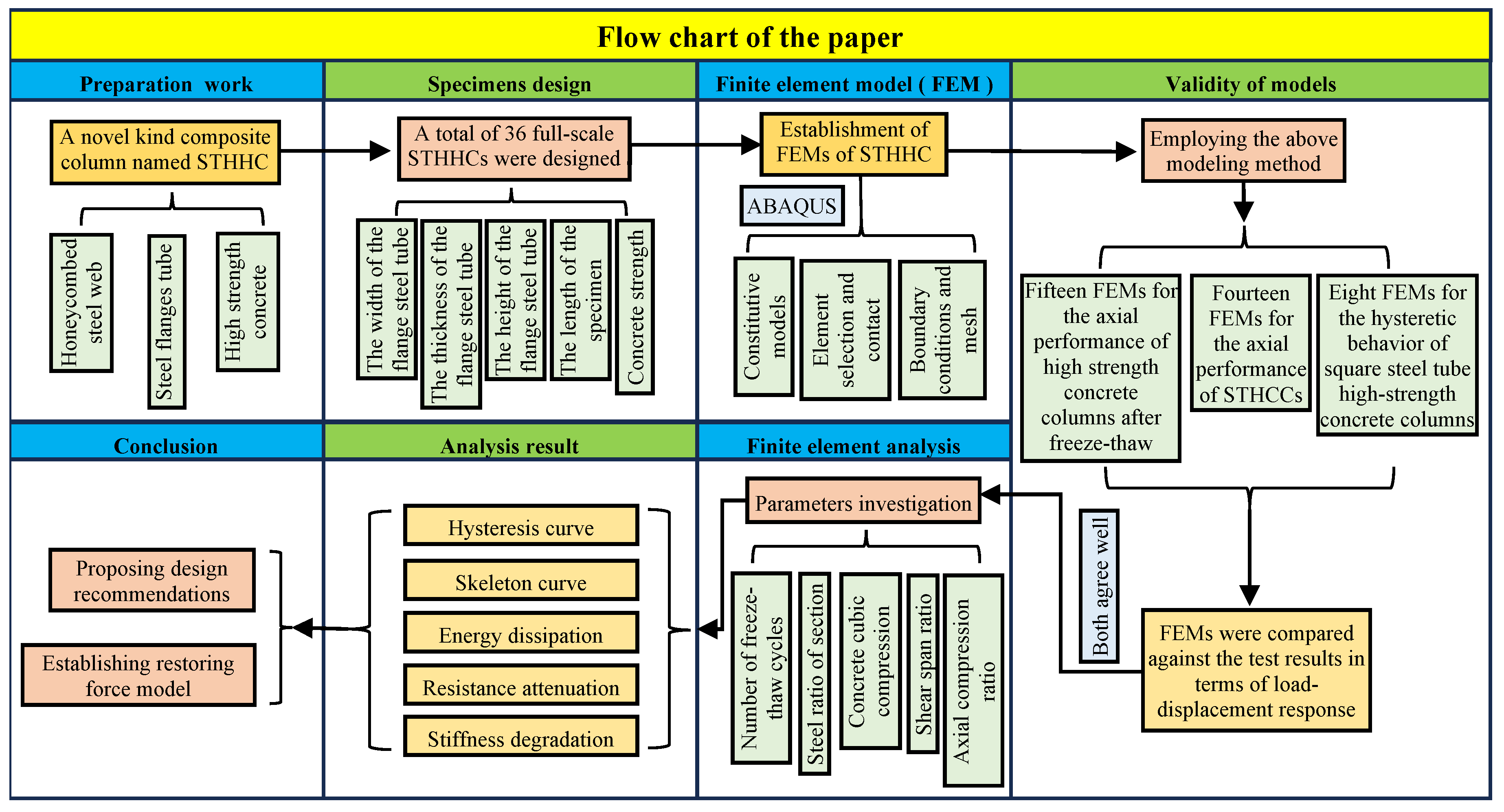
2. Analysis Process of the Paper

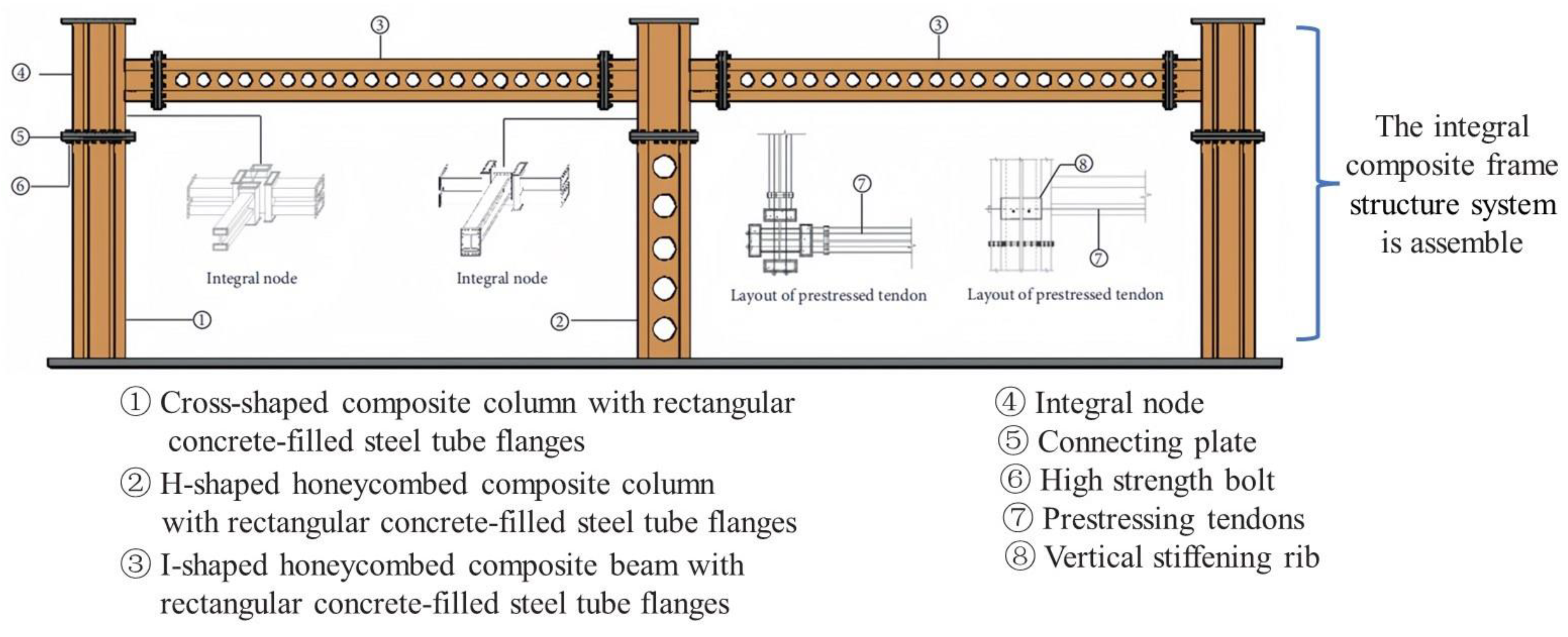
The main contents of this paper include specimen design, establishing finite element models, verifying the rationality of the model, parameter analysis, establishing the restoring force model, and proposing design recommendations. The detailed arrangement of the paper can be seen in Figure 2.

3. Specimen Design

To investigate the hysteresis performance of STHHCs, this paper refers to the experimental research on seismic behavior of ultrahigh-performance concrete-filled square steel tubular short columns by Wu et al. [28]. Their research suggests that the sectional steel ratio, the axial compression ratio, and the concrete strength have varying degrees of impact on the seismic performance of short columns.

A total of 36 full-scale STHHCs are designed, taking the shear span ratio (λ_s), the axial compression ratio (n₀), the number of freeze-thaw cycles (N_c), the concrete cubic compression strength (f_cu), and the steel ratio of the section (α_s) as the main parameters for this paper. The specific size and physical significance of the parameters can be seen in Figure 2 and

Table 1. The specific sizes and parameters of the specimens.

Specimens	b × h1 × hw × t1 /mm	L /mm	Nc	λs	n0	as /%	fcu /MPa
STHHC-1	500 × 320 × 400 × 4	2600	0	2.50	0.40	4.23	70
STHHC-2	500 × 320 × 400 × 4	2600	100	2.50	0.40	4.23	70
STHHC-3	500 × 320 × 400 × 4	2600	200	2.50	0.40	4.23	70
STHHC-4	500 × 320 × 400 × 4	2600	300	2.50	0.40	4.23	70
STHHC-5	500 × 320 × 400 × 6	2600	0	2.50	0.40	6.45	70
STHHC-6	500 × 320 × 400 × 6	2600	100	2.50	0.40	6.45	70
STHHC-7	500 × 320 × 400 × 6	2600	200	2.50	0.40	6.45	70
STHHC-8	500 × 320 × 400 × 6	2600	300	2.50	0.40	6.45	70
STHHC-9	500 × 320 × 400 × 8	2600	0	2.50	0.40	8.74	70
STHHC-10	500 × 320 × 400 × 8	2600	100	2.50	0.40	8.74	70
STHHC-11	500 × 320 × 400 × 8	2600	200	2.50	0.40	8.74	70
STHHC-12	500 × 320 × 400 × 8	2600	300	2.50	0.40	8.74	70
STHHC-13	500 × 320 × 400 × 4	2080	0	2.00	0.40	4.23	70
STHHC-14	500 × 320 × 400 × 4	2080	100	2.00	0.40	4.23	70
STHHC-15	500 × 320 × 400 × 4	2080	200	2.00	0.40	4.23	70
STHHC-16	500 × 320 × 400 × 4	2080	300	2.00	0.40	4.23	70
STHHC-17	500 × 320 × 400 × 4	3120	0	3.00	0.40	4.23	70
STHHC-18	500 × 320 × 400 × 4	3120	100	3.00	0.40	4.23	70
STHHC-19	500 × 320 × 400 × 4	3120	200	3.00	0.40	4.23	70
STHHC-20	500 × 320 × 400 × 4	3120	300	3.00	0.40	4.23	70
STHHC-21	500 × 320 × 400 × 4	2600	0	2.50	0.60	4.23	70
STHHC-22	500 × 320 × 400 × 4	2600	100	2.50	0.60	4.23	70
STHHC-23	500 × 320 × 400 × 4	2600	200	2.50	0.60	4.23	70
STHHC-24	500 × 320 × 400 × 4	2600	300	2.50	0.60	4.23	70
STHHC-25	500 × 320 × 400 × 4	2600	0	2.50	0.80	4.23	70
STHHC-26	500 × 320 × 400 × 4	2600	100	2.50	0.80	4.23	70
STHHC-27	500 × 320 × 400 × 4	2600	200	2.50	0.80	4.23	70
STHHC-28	500 × 320 × 400 × 4	2600	300	2.50	0.80	4.23	70
STHHC-29	500 × 320 × 400 × 4	2600	0	2.50	0.40	4.23	60
STHHC-30	500 × 320 × 400 × 4	2600	100	2.50	0.40	4.23	60
STHHC-31	500 × 320 × 400 × 4	2600	200	2.50	0.40	4.23	60
STHHC-32	500 × 320 × 400 × 4	2600	300	2.50	0.40	4.23	60
STHHC-33	500 × 320 × 400 × 4	2600	0	2.50	0.40	4.23	80
STHHC-34	500 × 320 × 400 × 4	2600	100	2.50	0.40	4.23	80
STHHC-35	500 × 320 × 400 × 4	2600	200	2.50	0.40	4.23	80
STHHC-36	500 × 320 × 400 × 4	2600	300	2.50	0.40	4.23	80

Note: b, h₁, h_w, and t₁ are the widths of web steel tube flanges, the sectional height of steel tube flanges, the widths of web and steel tube flanges, and the wall thicknesses of steel tube, respectively. L represents the length of STHHC, λ_s = L/(2h₁ + h_w).

. The yield strength of the steel (f_yk) for the flange steel pipe and honeycomb steel web plate is taken as 345 MPa, the thickness (t₂) of the honeycomb steel web is taken as 10 mm, and the aperture (d) and the hole spacing (s) of the honeycomb steel web are taken as 240 mm and 100 mm, respectively.

4. Finite Element Model (FEM)

4.1. Constitutive Models of Materials

To simulate the behavior of steel more accurately in the finite element analysis and to consider the influence of the plastic hardening effect of steel, a nonlinear constitutive model is selected for steel in this paper. An ideal elastic-plastic constitutive model is employed as the constitutive model (CM) of steel [29]. Q345 grade steel is used in the steel, with an elastic modulus of 2.06 × 10⁵ MPa and a density of 7850 kg/m³.

The constitutive model of concrete is the foundation of nonlinear analysis, considering the influence of plastic damage and constraint effects on the performance of concrete. Therefore, the nonlinear constitutive model of concrete—which is proposed by L.H. Han [30] and which considers the confinement effect—is employed as the confined constitutive model of concrete to simulate the stress process of concrete without freeze-thaw cycles, as shown in Figure 3. The density of concrete is taken as 2450 kg/m³.

The constrained concrete constitutive model as modified by K. Cao [31] is used to simulate the stress process of concrete in the process of finite element simulation, when the specimen undergoes freeze-thaw cycles. This model considers the influence of freeze-thaw cycles on the peak strain (ε₀) and peak stress (σ₀) of the core concrete, and the uniaxial σ-ε constitutive model of core concrete after freeze-thaw cycles is therefore proposed.

The expression is as follows:

(1)

The compression analysis stress-strain relationship expression is as follows:

$$y=\left\{\begin{array}{l}2x-x^2\cdots \cdots \cdots \cdots \cdots (x\le 1)\\ {\displaystyle \frac{x}{\beta {(x-1)}^{\eta }+x}}\cdots \cdots \cdots (x>1)\end{array}\right.$$

(1)

where, $x=\epsilon /{\epsilon }_0$, $y=\delta /{\delta }_0$.

$${\delta }_0=f_{\mathrm{c}}^{\prime }(1-0.065n)$$

(2)

$${\epsilon }_0=(1300+12.5f_{\mathrm{c}}^{\prime }+800{\xi }^{0.2})\times {10}^{-6}$$

(3)

$$\eta =1.6+{\displaystyle \frac{1.5}{x}}$$

(4)

$$\beta ={(f_{\mathrm{c}}^{\prime })}^{0.1}/[1.2\sqrt{1+\xi }]$$

(5)

where $f_{\mathrm{c}}^{\prime }$ is the compressive strength of concrete prism, n = N_c/100, and N_c is the number of freeze-thaw cycles.

(2)

The tensile stress-strain relationship formulation is as follows:

In ABAQUS, the stress fracture energy relationship (GFI) can be used to describe the tensile softening performance of concrete for tensile simulation. The cracking stress is taken as 1/10 of the ultimate compressive stress of concrete, and the fracture energy is calculated using Formula (6):

$$G_{\mathrm{f}}=a\cdot {\left({\displaystyle \frac{f_{\mathrm{c}}^{\prime }}{10}}\right)}^{0.7}\times {10}^{-3}({\mathrm{N}/\mathrm{mm}}^2)$$

(6)

where a = 1.25 d_max + 10, and d_max is coarse aggregate particle size.

When calculating, the elastic modulus of the concrete is determined according to Equation (7):

$$E_{\mathrm{c}}=4700\sqrt{f_{\mathrm{c}}^{\prime }}(\mathrm{MPa})$$

(7)

The elastic moduli of C60 concrete, C70 concrete, and C80 concrete in this article are taken as 3.11 × 10⁴ MPa, 3.34 × 10⁴ MPa, and 3.33 × 10⁴ MPa, respectively. The Poisson’s ratio of concrete in the elastic stage is taken as 0.2.

The constitutive model curves calculated according to the above formula are shown in Figure 3.

4.2. The Establishment of FEM

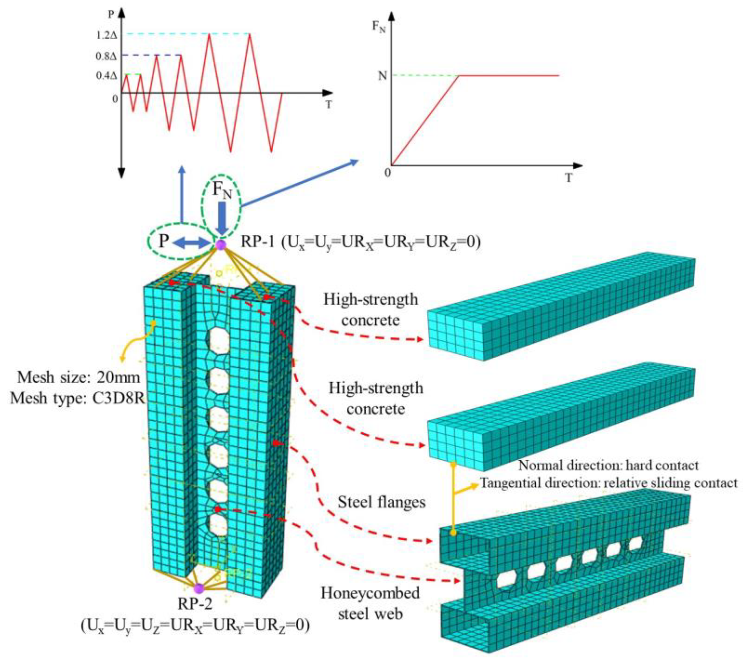
4.2.1. The Selection of Element and Contact

Finite element models of STHHC specimens are formed via the ABAQUS software. The concrete, steel webs, and steel tubes are all modeled using C3D8R elements. Universal contact is used to simulate the contact mode between concrete and the steel tubes. Hard contact is utilized in the normal direction, and relative sliding contact is utilized in the tangential direction, with a friction coefficient of 0.3 [32].

4.2.2. Boundary Conditions and Loading

Reference points RP-1 and RP-2 are set at the center points of the cross-section at both ends of the composite column, and the upper and lower surfaces are coupled with the reference points to ensure that the specimen’s surface can deform synergistically while applying axial load, avoiding bias pressure. Fixed boundary conditions are utilized on the upper surface of the composite column, and fully consolidated boundary conditions are utilized on the lower surface of the composite column, The loading process is separated into two parts. In the first analysis step, the axial load is applied. After the axial load remains unchanged, the second analysis step is carried out, which involves the horizontal reciprocating load in the form of displacement loading. The finite element model of STHHC is shown in Figure 4.

4.2.3. Grid Division

In order to guarantee calculation accuracy and enhance calculation speed, different grid sizes are set for the finite element models of STHCC-6 and STHCC-12 [33] as examples, and these models are then computed. By comparing the calculation results, it is found that a grid size of 20 mm is selected, and the results approximate the experimental values, as shown in Figure 5.

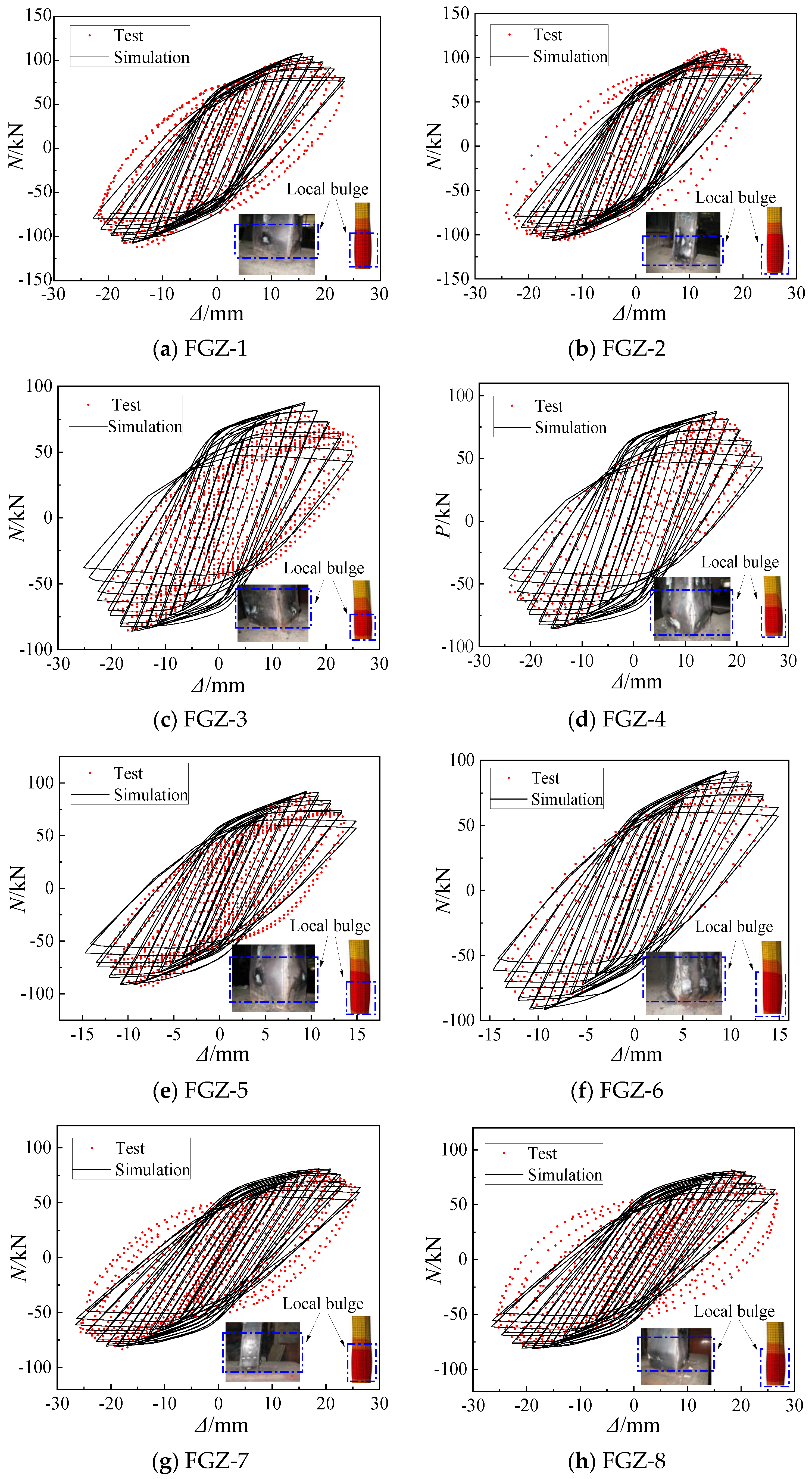
4.3. Experimental Verification of Finite Element Models

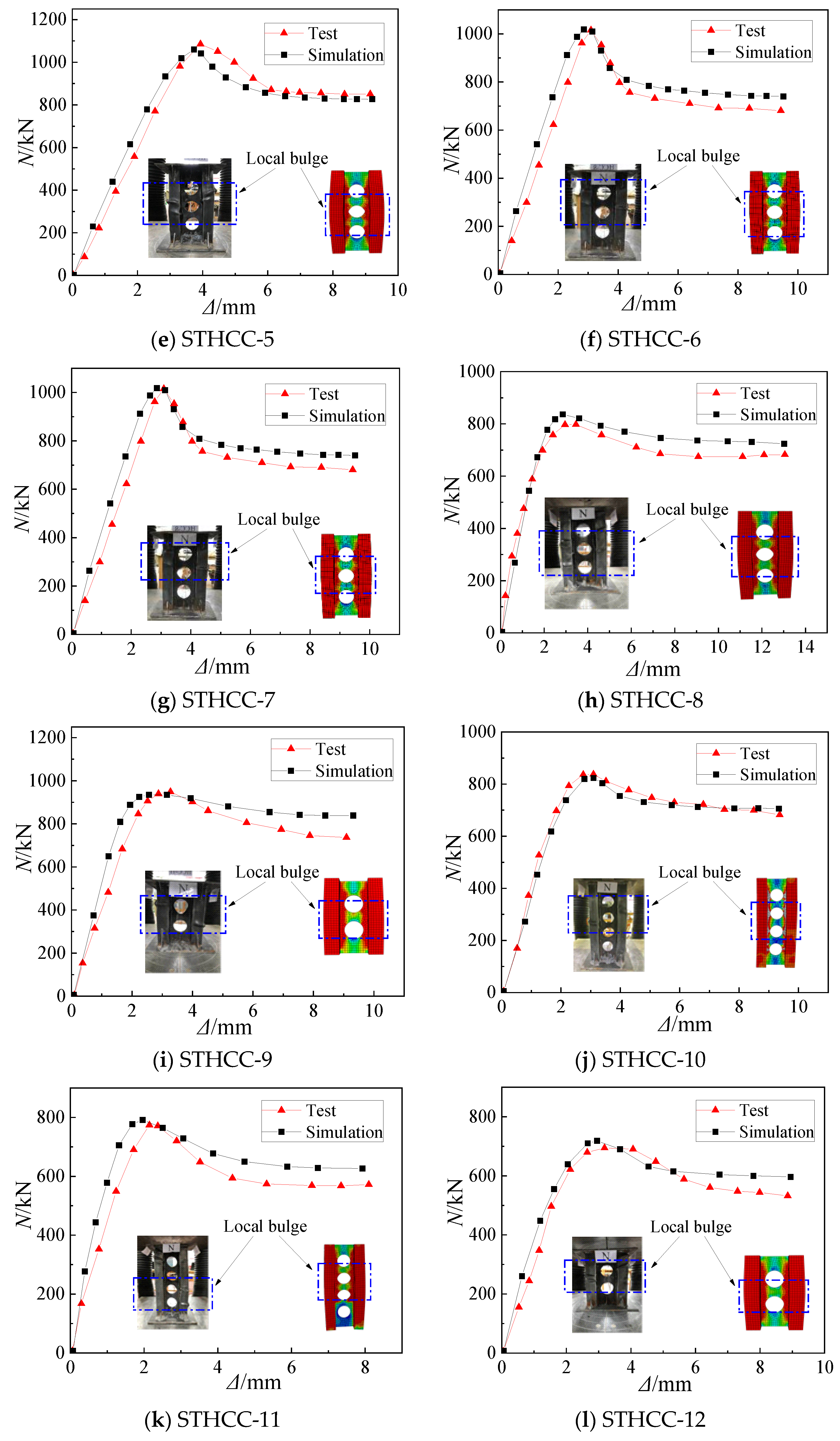
4.3.1. STHCC Model Validation

Numerical simulation for 14 existing rectangular steel tube concrete flanges honeycomb steel web composite short column (STHCC) specimens [33] is carried out via ABAQUS, and the specific parameters of all test specimens are shown in

Table 2. Parameters and test data of specimens.

Specimens	h1 × b × hw × t2 × t1 /mm	λ	l /mm	ξ	fyf /MPa	fcu /MPa	${\mathit{N}}_{\mathbf{U}}^{\mathbf{T}}$ /kN	${\mathit{N}}_{\mathbf{U}}^{\mathbf{S}}$ /kN	$\frac{\left|{\mathit{N}}_{\mathbf{U}}^{\mathbf{T}}-{\mathit{N}}_{\mathbf{U}}^{\mathbf{S}}\right|}{{\mathit{N}}_{\mathbf{U}}^{\mathbf{T}}}$/%
STHCC-1	50 × 100 × 100 × 6 × 1.7	12.82	370	0.60	269	49.50	740.0	763.4	3.17
STHCC-2	50 × 100 × 100 × 6 × 2.3	12.82	370	0.88	282	49.50	871.7	864.5	0.83
STHCC-3	50 × 100 × 100 × 6 × 3.8	12.82	370	1.60	286	49.50	1175.6	1150.8	2.11
STHCC-4	50 × 100 × 100 × 6 × 2.3	12.82	370	0.82	282	53.17	1070.4	1057.4	1.21
STHCC-5	50 × 100 × 100 × 6 × 2.3	12.82	370	0.66	282	55.69	1172.7	1152.3	1.73
STHCC-6	50 × 100 × 100 × 6 × 2.3	12.82	370	0.78	282	65.60	1015.9	1020.1	0.41
STHCC-7	50 × 100 × 100 × 8 × 1.7	12.82	370	0.60	269	49.50	752.6	789.6	4.91
STHCC-8	50 × 100 × 100 × 11 × 2.7	12.82	370	0.60	269	49.50	796.7	834.1	4.69
STHCC-9	50 × 100 × 100 × 6 × 2.3	9.35	270	0.88	282	49.50	947.0	936.9	1.06
STHCC-10	50 × 100 × 100 × 6 × 2.3	16.28	470	0.88	282	49.50	841.1	829.0	1.36
STHCC-11	50 × 100 × 100 × 6 × 1.7	9.35	270	0.60	269	49.50	772.9	787.8	1.93
STHCC-12	50 × 100 × 100 × 6 × 1.7	16.28	470	0.60	269	49.50	741.1	762.8	2.92
STHCC-13	50 × 100 × 100 × 6 × 3.8	9.35	270	1.60	286	49.50	1276.0	1299.1	1.81
STHCC-14	50 × 100 × 100 × 6 × 3.8	16.28	470	1.60	286	49.50	1069.0	1080.5	1.07

Note: b, t₁, t₂, h₁, and h_w are the width of the web steel tube flanges, the thicknesses of the steel tube wall, the thickness of the honeycomb steel web, the height of the steel tube flanges section, and the widths of the webs, respectively. The physical meanings of other variables can be found in reference [33].

. The load-displacement (N-Δ) curves of STHCC specimens are obtained, as shown in Figure 6. As is indicated in Figure 6, the curves obtained from finite element simulation are in good agreement with the experimental curves. A comparison between the simulation results ($N_{\mathrm{U}}^{\mathrm{S}}$) and the experimental data ($N_{\mathrm{U}}^{\mathrm{T}}$) is shown in Figure 7. It can be seen in Figure 7 that the two are in good agreement with a maximum error (Error_max) of 4.91%, indicating that the finite element model established in this paper can accurately simulate the stress process of this new kind of composite column.

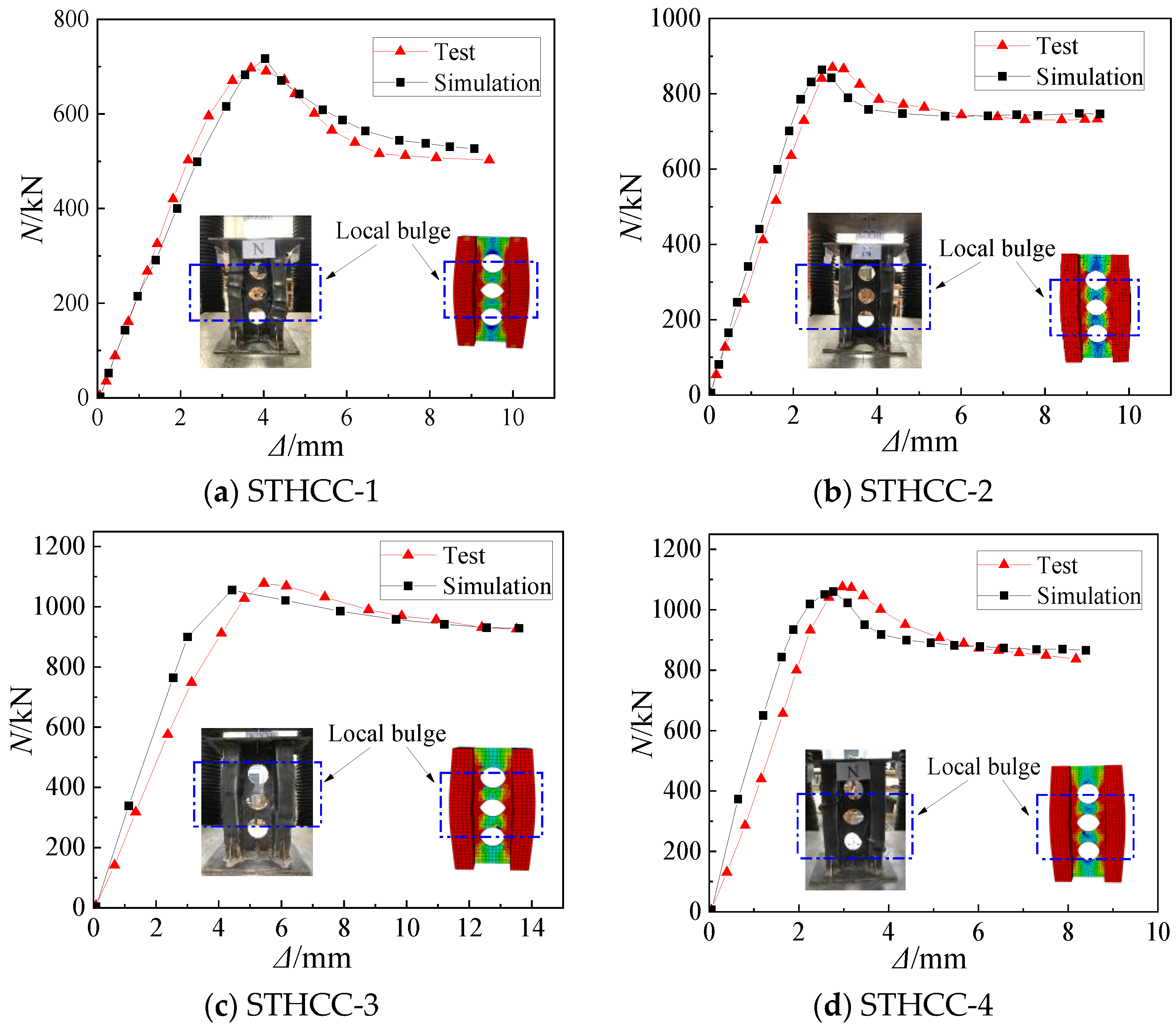
4.3.2. Model Validation of Short Columns with Concrete-Filled Square Steel Tubes

Numerical simulation for the 12 existing test specimens of short columns with concrete-filled steel tubes after freeze-thaw cycles [34] is conducted through ABAQUS software. The specific parameters of all test specimens are shown in

Table 3. Parameters and test data of specimens.

Specimens	D /mm	L /mm	t /mm	fcu /MPa	α	fy /MPa	${\mathit{N}}_{\mathbf{U}}^{\mathbf{T}}$ /kN	${\mathit{N}}_{\mathbf{U}}^{\mathbf{S}}$ /kN	$\frac{\left|{\mathit{N}}_{\mathbf{U}}^{\mathbf{T}}-{\mathit{N}}_{\mathbf{U}}^{\mathbf{S}}\right|}{{\mathit{N}}_{\mathbf{U}}^{\mathbf{T}}}$/%
SC2-0	100	300	2.06	63.7	0.113	338.4	808.38	834.96	3.34
SC2-100	100	300	2.06	63.7	0.113	338.4	783.77	802.04	2.32
SC2-200	100	300	2.06	63.7	0.113	338.4	808.99	832.09	2.83
SC2-300	100	300	2.06	63.7	0.113	338.4	749.10	775.16	3.41
S2-0	100	300	2.00	83.9	0.085	184.7	861.67	814.23	5.83
S2-100	100	300	2.00	83.9	0.085	184.7	783.92	778.60	0.68
S2-200	100	300	2.00	83.9	0.085	184.7	777.55	754.89	3.00
S2-300	100	300	2.00	83.9	0.085	184.7	663.06	715.48	7.91
S3-0	100	300	3.00	83.9	0.132	176.5	891.58	856.82	4.06
S3-100	100	300	3.00	83.9	0.132	176.5	775.53	800.38	3.20
S3-200	100	300	3.00	83.9	0.132	176.5	754.48	815.90	8.14
S3-300	100	300	3.00	83.9	0.132	176.5	722.31	772.20	6.91

Note: D, T, and L are the cross-sectional width of the steel tube, the thickness of the steel tube, and the length of the specimen, respectively. The physical meanings of other variables are found in reference [34].

. The load-displacement (N-Δ) curves of specimens are obtained, and several representative N-Δ curves are selected, as shown in Figure 8. As is indicated in Figure 8, the curves obtained from finite element simulation match well with the experimental curves. The comparison between the simulation data ($N_{ \mathrm{U}}^{ \mathrm{S}}$) and the experimental data ($N_{ \mathrm{U}}^{ \mathrm{T}}$) is shown in Figure 7. As shown in Figure 7, it can be observed that the two are in close accordance with an Error_max of 8.14%, indicating that the finite element model of short columns established in this paper can precisely simulate the stress process of this new kind of composite column.

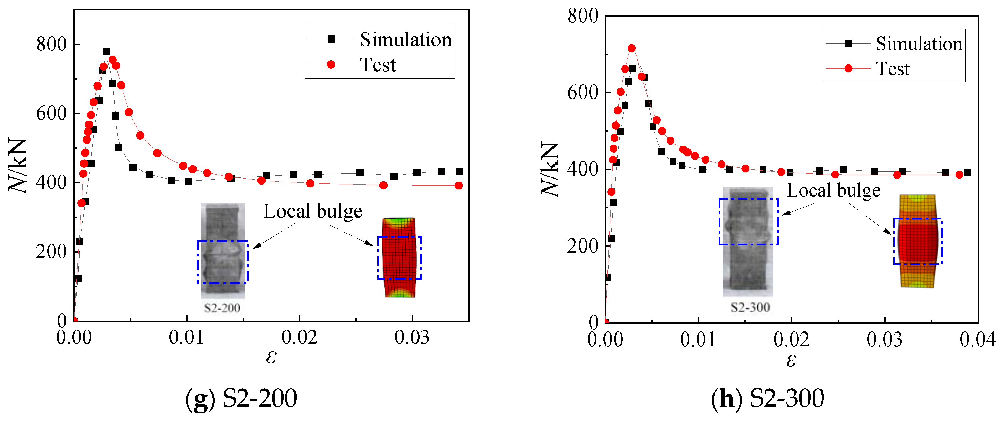
4.3.3. Model Validation of High-Strength Concrete Columns with Square Steel Tubes

Numerical simulation for 8 existing test specimens of square steel tube concrete columns [35] is conducted via the finite element software ABAQUS. The specific test parameters of the specimens are shown in

Table 4. Parameters and experimental data of specimens.

Specimens	B × t × L /mm	λ	α	nt	fy /MPa	fcu,k /MPa	${\mathit{N}}_{\mathbf{U}}^{\mathbf{T}}$ /kN	${\mathit{N}}_{\mathbf{U}}^{\mathbf{S}}$ /kN	$\frac{\left|{\mathit{N}}_{\mathbf{U}}^{\mathbf{T}}-{\mathit{N}}_{\mathbf{U}}^{\mathbf{S}}\right|}{{\mathit{N}}_{\mathbf{U}}^{\mathbf{T}}}$/%
FGZ-1	150 × 5.5 × 900	12.82	0.165	0.5	291.8	65.1	108.3	111.3	2.78
FGZ-2	150 × 5.5 × 900	12.82	0.165	0.5	291.8	65.1	112.1	111.3	0.72
FGZ-3	150 × 3.1 × 900	12.82	0.088	0.5	252.6	65.1	83.4	87.6	5.03
FGZ-4	150 × 3.1 × 900	12.82	0.088	0.5	252.6	65.1	82.1	87.6	6.70
FGZ-5	150 × 5.5 × 900	12.82	0.165	0.7	291.8	65.1	85.2	91.2	7.04
FGZ-6	150 × 5.5 × 900	12.82	0.165	0.7	291.8	65.1	84.1	91.2	8.44
FGZ-7	150 × 5.5 × 1250	12.82	0.165	0.5	291.8	65.1	87.9	89.7	2.04
FGZ-8	150 × 5.5 × 1250	12.82	0.165	0.5	291.8	65.1	83.3	89.7	7.68

Note: B, L, and t are the cross-sectional width of the steel tube, the length of the specimen, and the thickness of the steel tube wall, respectively. The physical meanings of other variables are found in reference [35].

. The hysteresis curves are obtained, as shown in Figure 9. As is indicated in Figure 9, the curves obtained from finite element simulation are in good agreement with those obtained from experiments, As can be seen in Figure 7, the two were in good agreement, with an Error_max of 8.44%, and therefore the finite element model established in this paper can accurately simulate the stress process of this new kind of composite column.

5. Parameter Investigation

5.1. Hysteresis Curves

The hysteresis curves of 36 specimens are obtained through finite element calculation, and several representative hysteresis curves are selected, as shown in Figure 10. As is seen in Figure 10, the hysteresis curves of all specimens before and after freeze-thaw show an ideal shuttle shape, demonstrating that the STHHC has both a good energy dissipation ability and freeze-thaw resistance. The specimens undergo elastic deformation at the beginning of loading, and the N-Δ curve gradually rises along a straight line. As the horizontal load gradually increases, the N-Δ curve exhibits nonlinear characteristics, and the deformation amplitude of the specimens gradually increases and enters the stage of elastic-plastic deformation. As the horizontal load gradually reaches the yield load, the specimens begin to experience stiffness degradation, and with the increase in loading times the stiffness degradation becomes more pronounced. At this point, the area of the hysteresis loop increases, and the shape of the hysteresis loop becomes fuller.

5.2. Skeleton Curves

To express it clearly, the abscissa of the skeleton curve of the specimens with 100, 200, and 300 freeze-thaw cycles is shifted to the right by 50 mm, 100 mm, and 150 mm, respectively. As depicted in Figure 11, the overall tendency of the skeleton curves is essentially the same. The change process of the skeleton curve can be separated into four stages: the elastic stage, elastic-plastic stage, descent stage, and failure stage. The first stage is the elastic stage, in which the skeleton curves present an oblique straight line state, with almost no change in the slope of the straight line. The second stage is the elastic-plastic stage, in which as the displacement load gradually increases, the bearing capacity of the composite column gradually reaches its peak. The third stage is the descending stage, where the bearing capacity of the composite column gradually decreases. However, under the constraint of the steel tube, the overall composite columns remain undamaged, and the deformation gradually intensifies at the column base. The fourth stage is the failure stage, where the bearing capacity of the specimen gradually decreases and where there is bulging deformation at the column base. When the skeleton curves drop to 85% of the peak value, it is considered a composite column failure. In addition, as the N_c increases, the horizontal peak load of the specimen gradually decreases. As is indicated in Figure 11a, the decrease in horizontal peak load is more significant with the increase of the α_s. As seen in Figure 11b, as the f_cu increases, the horizontal peak load of the specimen gradually increases. Figure 11c shows that as the λ_s increases, the horizontal peak load of the specimen gradually decreases. Figure 11d demonstrates that with the increase in the n₀, the horizontal peak load of the specimen gradually increases, while the augmentation in its peak load is relatively small.

5.3. Energy Dissipation Capacity

The equivalent viscous damping coefficient is used as an indicator to evaluate the energy dissipation capacity of composite columns [36], and its calculation expression and calculation diagram are illustrated in in Equation (8) and Figure 12, respectively.

$$h\mathrm{e}={\displaystyle \frac{1}{2\mathsf{\pi }}}\times {\displaystyle \frac{S_{\left(\mathrm{ABC}+\mathrm{CDA}\right)}}{S_{\left(\mathsf{\Delta }\mathrm{OBE}+\mathsf{\Delta }\mathrm{ODF}\right)}}}$$

(8)

To express it clearly, the abscissa of the h_e-Δ curve of the specimens with 100, 200, and 300 freeze-thaw cycles is shifted to the right by 50 mm, 100 mm, and 150 mm, respectively. Figure 13 shows that after freeze-thaw cycles, the curve trends of each composite column under low-cycle horizontal reciprocating loads are basically consistent. With the increase in the horizontal displacement, the equivalent viscous damping coefficient gradually increases, but the rate of increase gradually slows down. As the N_c increases, the equivalent viscous damping coefficient of specimens changes less, and the impact on the energy dissipation capacity of the specimens is relatively miniscule. All specimens show an excellent energy dissipation ability. Figure 13a shows that as the α_s increases, the equivalent viscous damping coefficient of the specimen also increases. Figure 13b illustrates that as the f_cu increases, the equivalent viscous damping coefficient of the specimen also gradually increases. Figure 13c shows that with an increasing λ_s, the equivalent viscous damping coefficient of the composite column decreases significantly. As seen in Figure 13d, with an increase in n₀, the equivalent viscous damping coefficient of the specimen gradually decreases. At the same time, as the axial compression ratio increases, the growth rate of the equivalent viscous damping coefficient in the later stage of loading slows and the decrease amplitude grows greater.

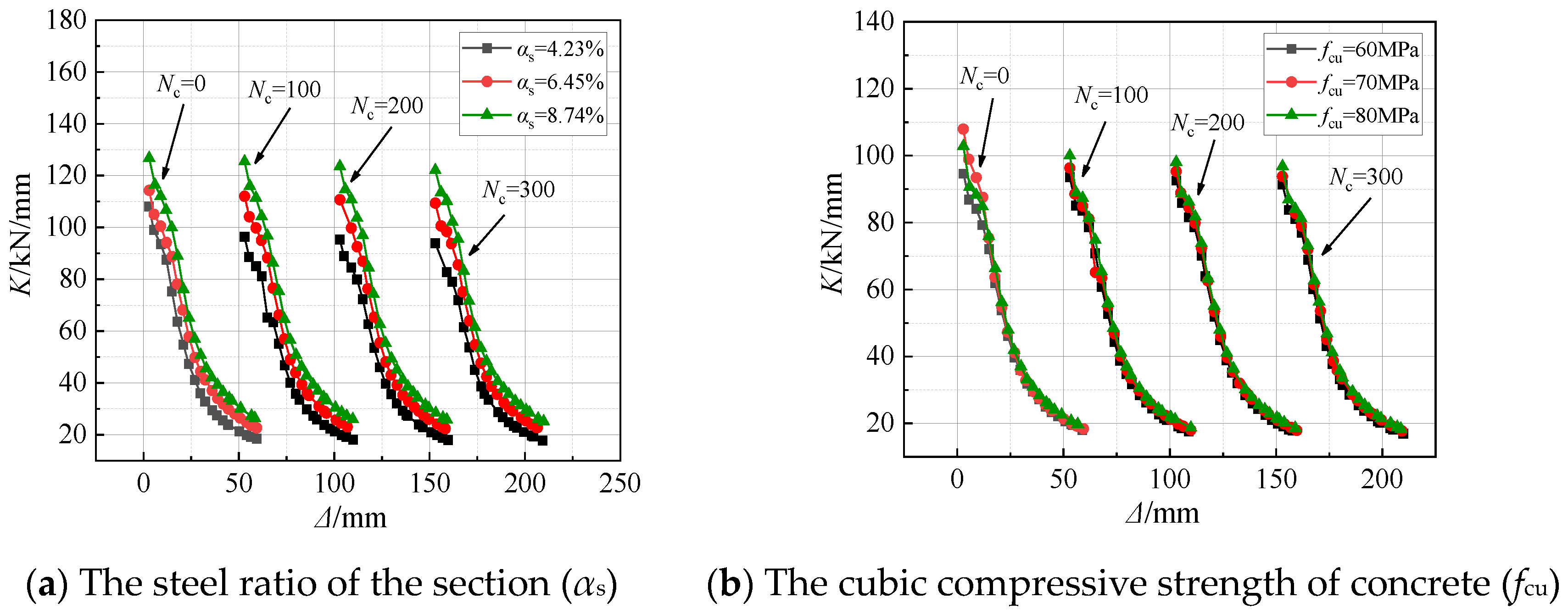
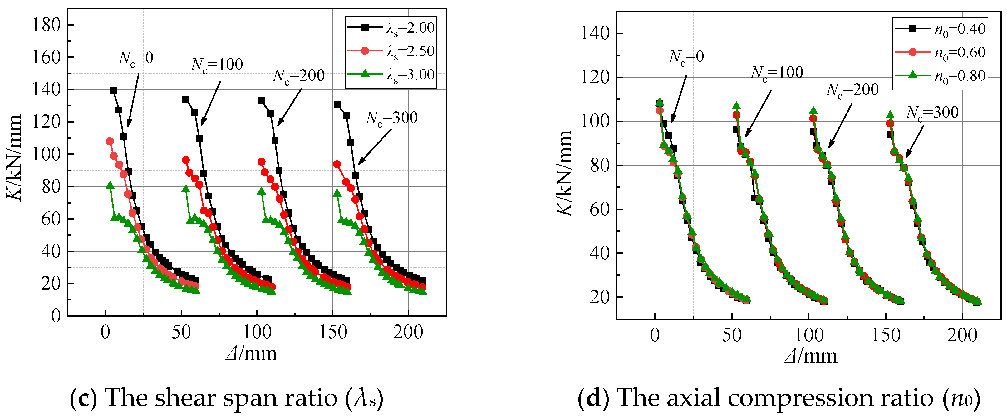
5.4. Stiffness Degradation

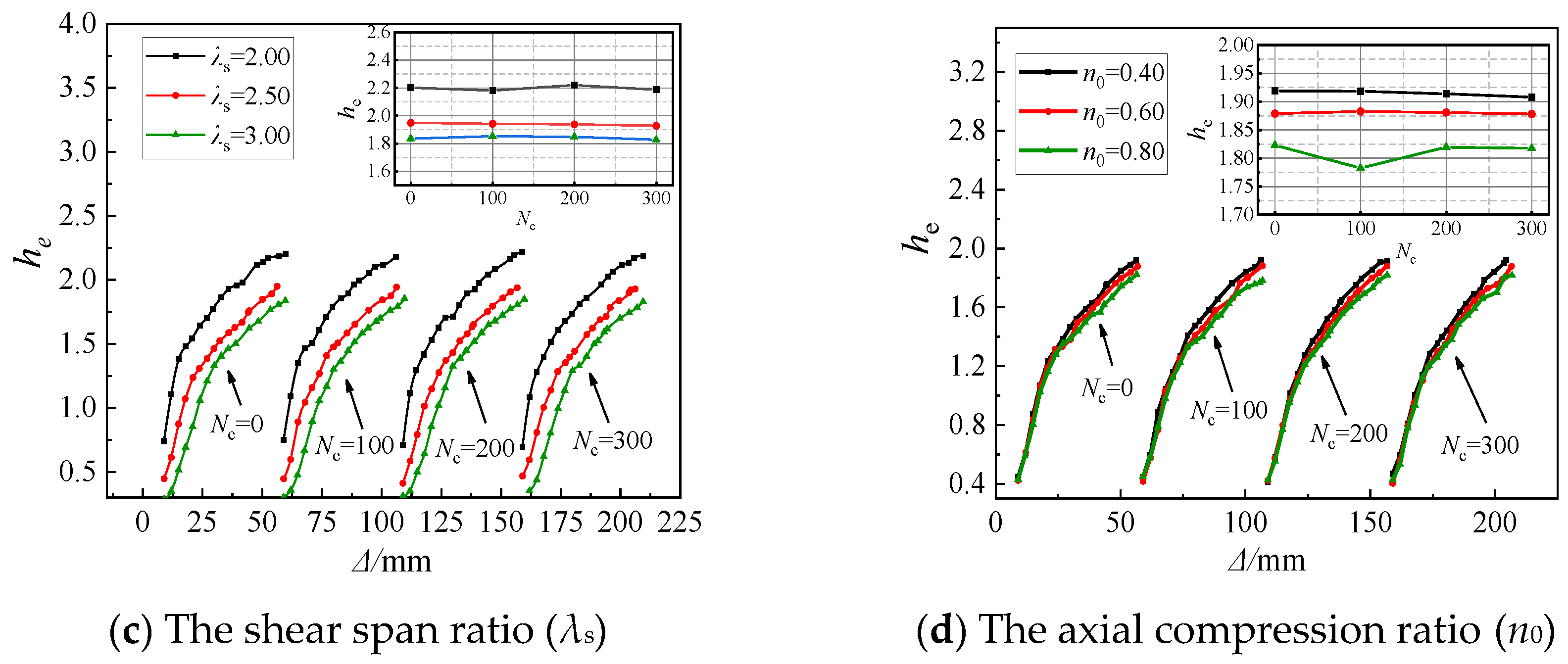
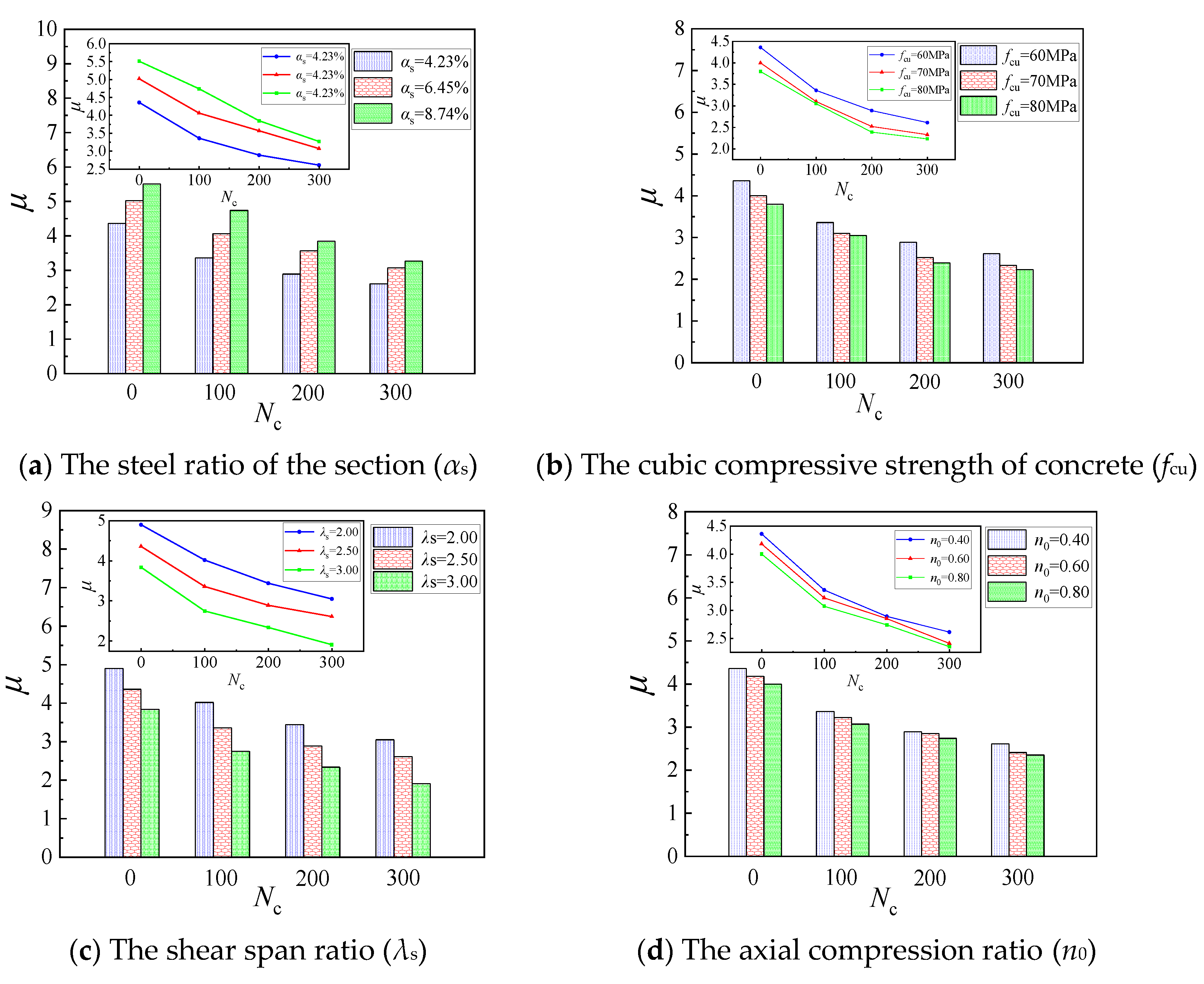
This paper aims to reveal the stiffness degradation phenomenon of specimens through the variation of secant stiffness during the loading process [37]. The calculation expression of secant stiffness K is shown in Equation (9).

$$K={\displaystyle \frac{\left|+P_{\mathrm{i}}\right|+\left|-P_{\mathrm{i}}\right|}{\left|+{\Delta }_{\mathrm{i}}\right|+\left|-{\Delta }_{\mathrm{i}}\right|}}$$

(9)

where, +Δ_i, −Δ_i, +P_i, and −P_i represent the displacement magnitude of the ith forward loading, the displacement magnitude of the i th reverse loading, the peak load magnitude corresponding to the i th forward cycles, and the peak load magnitude corresponding to the i th reverse cycles, respectively.

As depicted in Figure 14, all specimens exhibit stiffness degradation after freeze-thaw cycles, and with the increase of the freeze-thaw cycles, the initial stiffness of specimens gradually decreases. It is indicated in Figure 14a that the initial stiffness of the specimen gradually increases with the increase of the α_s. It is indicated in Figure 14b that as the f_cu gradually increases, the stiffness of the specimens gradually increases. It is indicated in Figure 14c that as the λ_s increases, the specimen’s stiffness decreases significantly, and specimens with larger shear span ratios experience more significant stiffness degradation during the initial loading stage. It is indicated in Figure 14d that as the n₀ increases, the initial stiffness of the specimen improves significantly. The stiffness degradation trend of specimens under different n₀ is not significantly different after freeze-thaw cycles.

5.5. Ductility

Ductility (μ) is a significant parameter for measuring the deformation capacity of specimens [38], and its expression is as follows:

$$\mu ={\displaystyle \frac{{\Delta }_{\mathrm{u}}}{{\Delta }_{\mathrm{y}}}}$$

(10)

where Δ_y is the yield displacement and Δ_u is the ultimate displacement.

The energy equivalent approach is employed to determine the yield displacement of the component, and the ultimate displacement is the displacement corresponding to the load dropping to 85% of the peak load in this paper, as shown in Figure 15.

After freeze-thaw cycles, all specimens exhibit good ductility. Figure 16 shows that as the N_c increases, the displacement ductility coefficient of specimens gradually decreases. Figure 16a indicates that as the α_s increases, the displacement ductility coefficient of the specimen significantly increases. As shown in Figure 16b, as the f_cu increases, the displacement ductility coefficient of specimens gradually decreases. Figure 16c shows that as the λ_s increases, the displacement ductility coefficient significantly decreases. Figure 16d shows that as the n₀ increases, the displacement ductility coefficient of specimens gradually decreases, and the change in the n₀ has little influence on the displacement ductility coefficient of specimens.

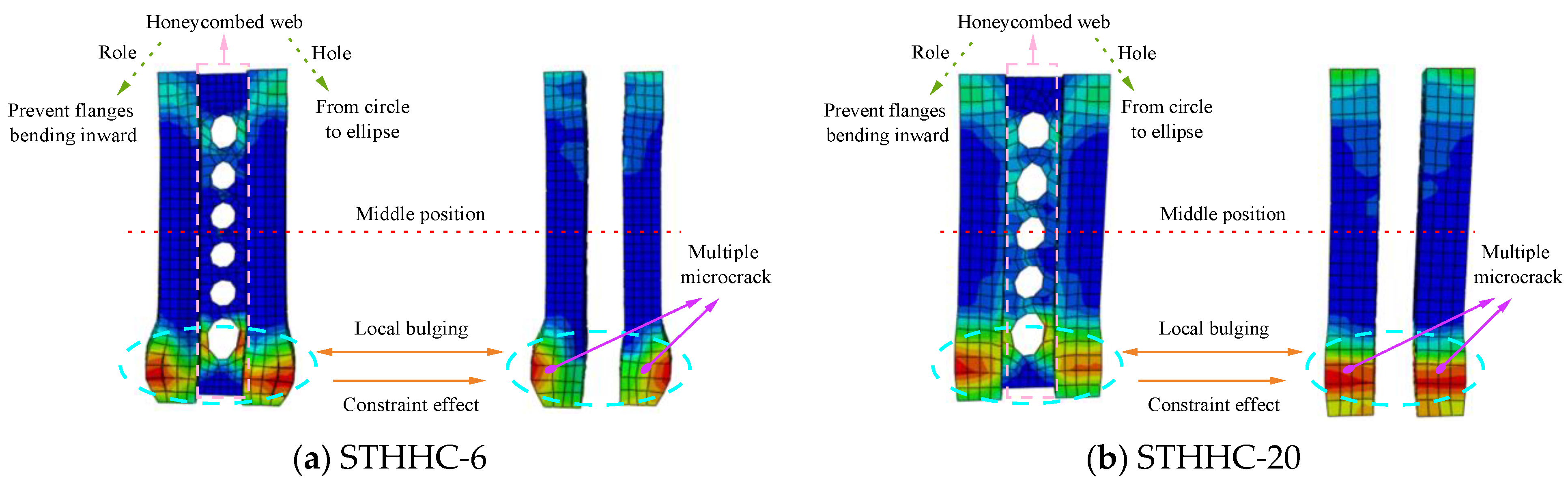
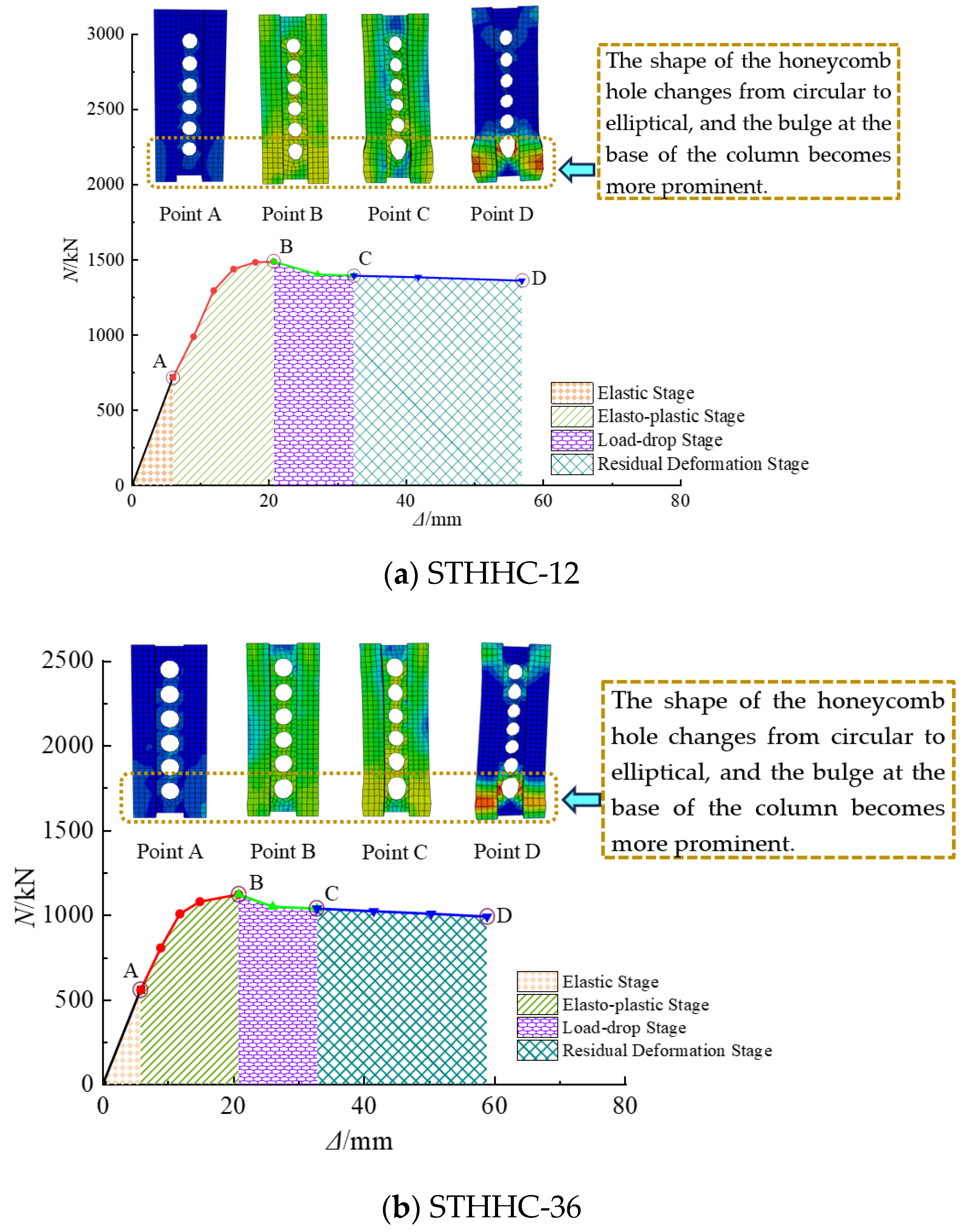
5.6. The Failure Mode of the Specimens

The failure mode of this new kind of composite column under low-cycle reciprocating loads is roughly similar after freeze-thaw cycles. This paper presents plastic deformation diagrams of several typical specimens, as depicted in Figure 17. Additionally, Figure 18 depicts the positive part of the skeleton curve of the STHHCs and the schematic diagram of the process failure in four stages. The specimen is found to easily undergo an overall bending deformation, with significant plastic deformation at the column base and relatively small plastic deformation in the remaining parts. After being subjected to axial and horizontal forces, the honeycomb steel web plate in the center of the composite column undergoes buckling deformation, causing the shape of the honeycomb hole to change from circular to elliptical. The deformation of the honeycomb hole at the column base is pronounced, indicating that the honeycomb steel web plate provides a certain amount of support to the inner side of the flange. The steel tube provides a restrictive influence on the core concrete, enhancing the deformation ability of the specimen. The concrete has a particularly supportive impact on the steel tubes, delaying the deformation. The maximum stress for the steel tubes and the concrete takes place at the column base. The core concrete at the column base undergoes vertical compression deformation and an obvious bulging deformation.

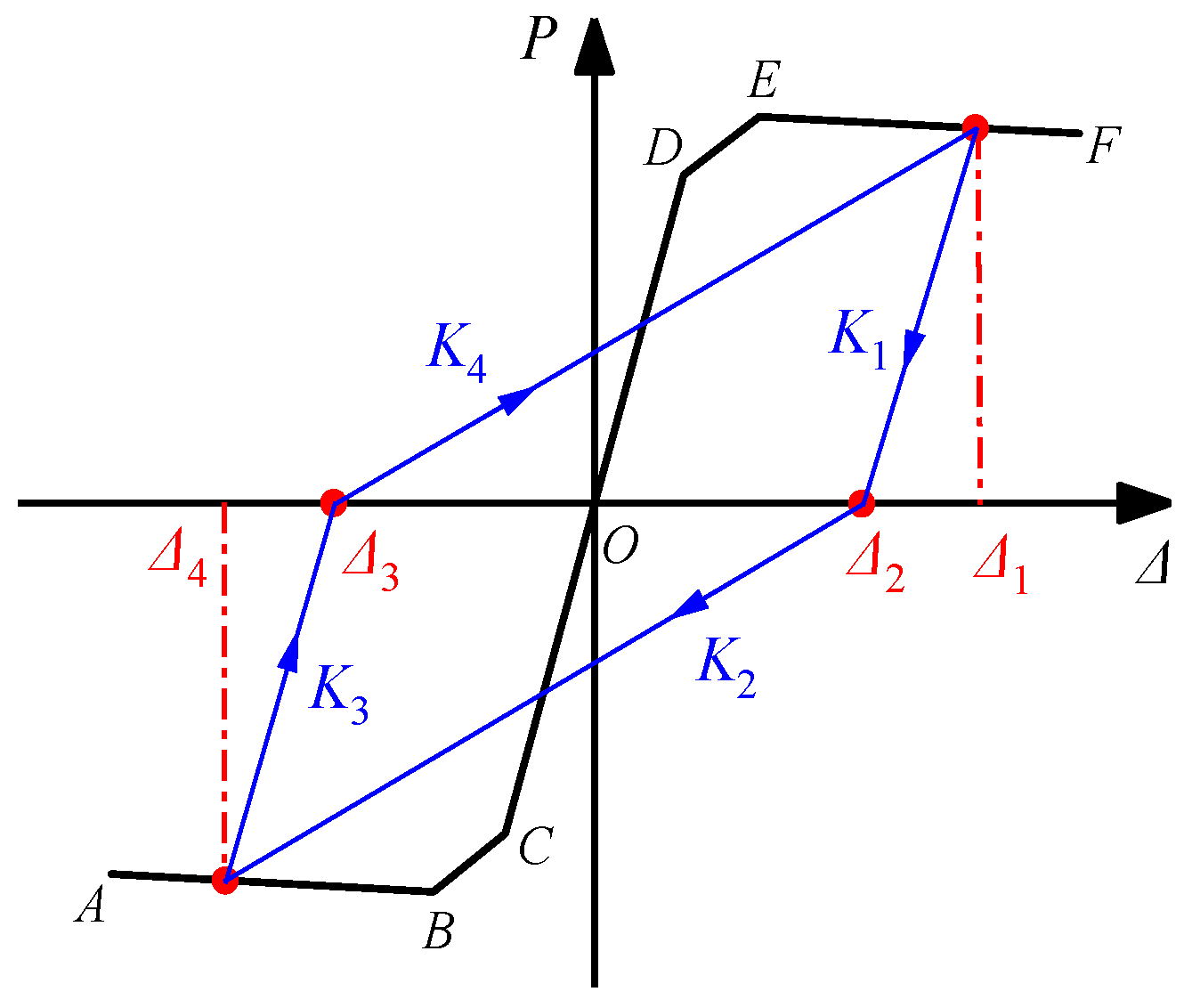
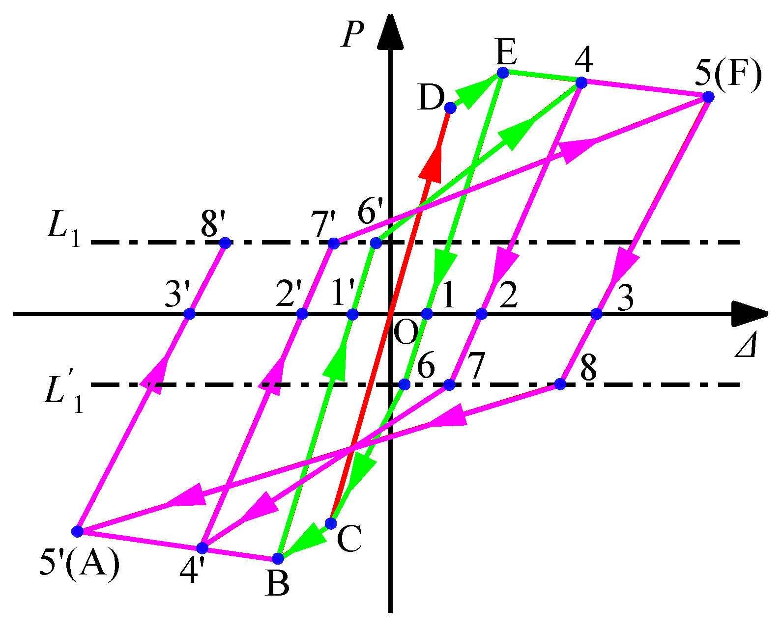
6. The Restoring Force Model

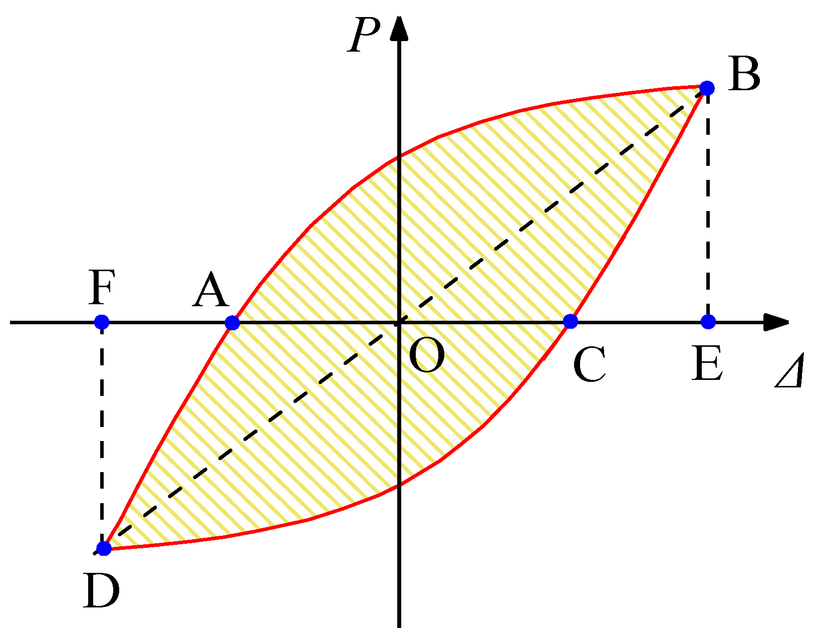
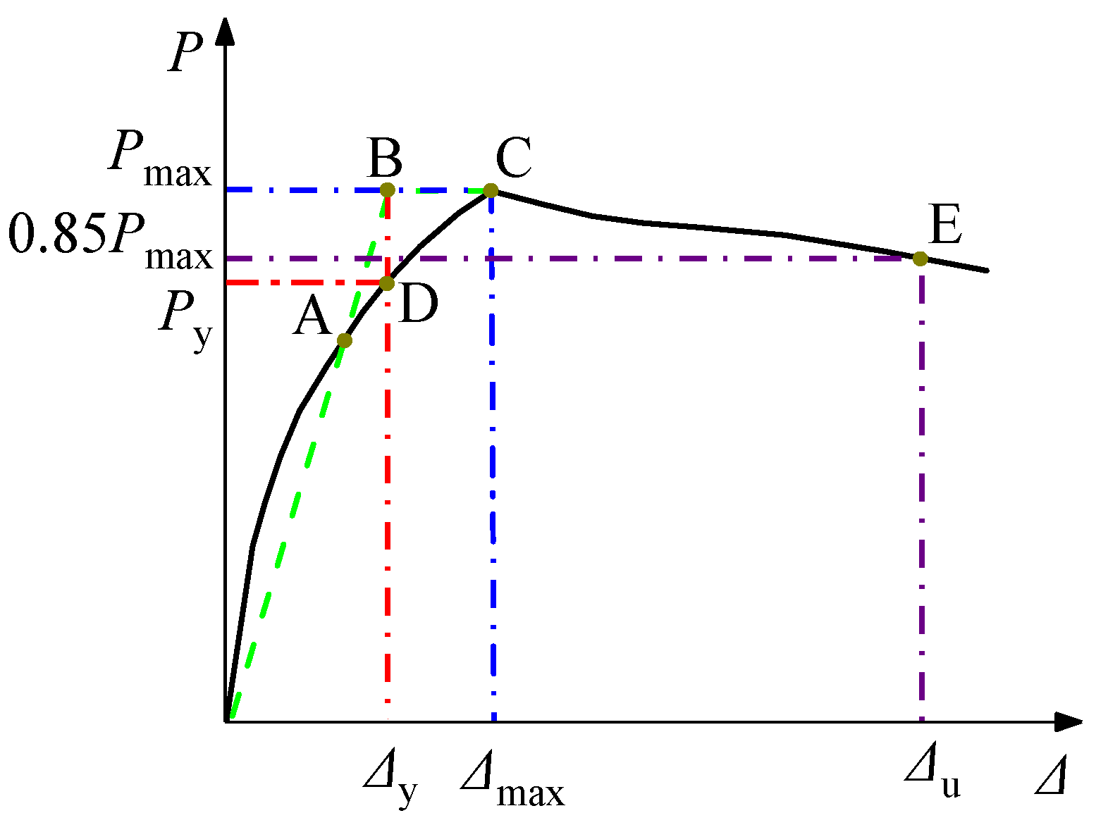
6.1. The Simplified Trilinear Skeleton Curve Model

The skeleton curves of all specimens are simplified for trilinear skeleton curves [39,40], shown in Figure 19, and the calculation equations are shown in

Table 5. The calculation equation of skeleton curves for the different stages.

Section	Regression Equation	Slope
OD	P/P+max = 4.604(Δ/Δ+max)	4.604
DE	P/P+max = 0.97(Δ/Δ+max) + 0.669	0.970
EF	P/P+max = −0.0657(Δ/Δ+max) + 1.022	−0.066
OC	P/|P−max| = 4.608(Δ/|Δ−max|)	4.608
CB	P/|P−max| = 1.007(Δ/|Δ−max|) − 0.664	1.007
BA	P/|P−max| = −0.0688(Δ/|Δ−max|) − 1.023	−0.069

Note: P⁺_max, P^–_max, Δ⁺_max, and Δ^–_max represent the positive peak, load the negative peak load, the displacement corresponding to the positive peak, and the displacement corresponding to the negative peak, respectively.

. In Figure 19, points C and D represent the yield points in the negative and positive directions, respectively, points B and E represent the peak points in the negative and positive directions, respectively, and points A and F represent the failure points in the negative and positive directions, respectively.

6.2. Degradation Law of Stiffness

From the hysteretic curves in Figure 10, it is observed that with the increase in loading displacement (Δ), the residual deformation increases by degrees and the stiffness degradation phenomenon becomes more apparent after the specimen yields. Figure 20 illustrates the degradation law of stiffness for STHHCs. K₁ and K₃ represent the positive unloading stiffness and the negative unloading stiffness, respectively, which are fitted using the logarithmic function. K₂ and K₄ represent the negative loading stiffness and positive loading stiffness respectively, which are fitted using the power function and the logarithmic function, respectively. The regression equations of stiffness for STHHCs are shown in

Table 6. The regression equations of stiffness for STHHCs.

Stage	Regression Equation	R2
Positive unloading	K1/K+0 = 0.8176(Δ1/Δ+max)−0.4496	0.8577
Negative loading	K2/K−0 = −1.982ln(Δ2/Δ+max + 0.0028) + 0.1774	0.9109
Negative unloading	K3/K−0 = 0.6339(Δ3/Δ−max)−0.1434	0.8200
Positive loading	K4/K+0 = 0.3344(Δ4/Δ−max)−1.0348	0.8506

Note: K⁺₀ and K⁻₀ represent the positive and negative initial loading stiffness, respectively. K⁺₀ and K⁻₀ are constants. Δ₁ and Δ₄ represent the displacement corresponding to positive and negative unloading points, respectively. Δ₂ and Δ₃ represent the residual displacement after positive and negative unloading, respectively.

. The degradation laws of stiffness for STHHCs at different stages are shown in Figure 21.

6.3. Restoring Force Model

Considering the characteristics of the skeleton curves, as well as the stiffness degradation law and hysteresis characteristics, the restoring force model of the composite columns is proposed, as depicted in Figure 22. In the model, D and C represent positive and negative yield points, while E and B represent positive and negative peak points and AB and EF represent positive and negative damage segments. In the model, the horizontal auxiliary lines L₁ and L′₁ are straight lines P = 0.30 P_m [41], and the auxiliary lines L₁ and L′₁ are symmetrical about the horizontal coordinate axis.

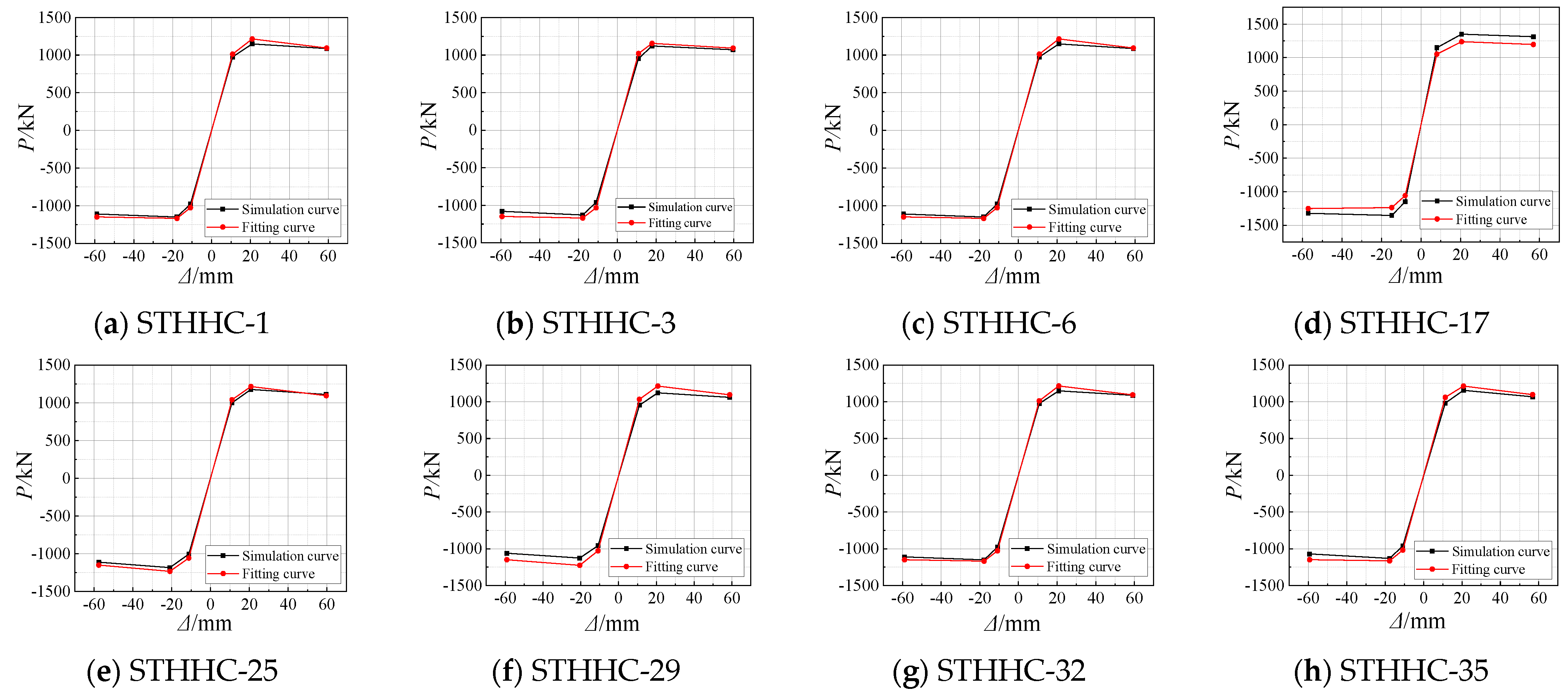
6.4. Comparison of Skeleton Curves

The skeleton curve model is used to calculate the skeleton curves of the specimens and compare them with the simulated value. The comparison outcomes of certain specimens selected are depicted in Figure 23. Figure 23 clearly shows that the regression value is in good accordance with the simulated value, showing good consistency and implying that the skeleton curve determined via the above method can better reflect the load–displacement relationship of the specimen.

6.5. Comparison of Hysteresis Curves

The above restoring force model is used to calculate the hysteresis curve of the STHHC specimens. By comparing the fitting curves with the simulation curves, it is found that the two are in good agreement, as shown in Figure 24.

6.6. Design Recommendations

In this paper, and taking as the main parameters the shear span ratio (λ_s), the axial compression ratio (n₀), the number of freeze-thaw cycles (N_c), the cubic compressive strength of concrete (f_cu), and the steel ratio of the section (α_s), the effects of different parameters on the hysteretic curve, skeleton curve, energy dissipation capacity, stiffness degradation and ductility of the composite column are studied. Based on the analysis of the seismic behavior of STHHCs after freeze-thaw cycles and the impact of varying parameters on the mechanical properties, the following conclusions are drawn and design recommendations are proposed:

(1)

As the steel ratio of the section increases, both the peak load and the ductility of the composite column’s horizontal bearing capacity significantly enhance. However, the increase in the steel ratio of the section has minimal influence on the column’s energy dissipation capacity. Therefore, a steel ratio of the section between 4.23% and 6.45% is recommended.

(2)

As the concrete strength increases, the composite column’s peak load and energy dissipation capacity improve. However, excessively high concrete strength leads to rapid load decay and reduced ductility after freeze-thaw cycles. The recommended cubic compressive strength of concrete is 70 MPa.

(3)

As the shear span ratio increases, the composite column’s secant stiffness at the beginning of loading significantly decreases, leading to a reduction in energy dissipation capacity and peak horizontal bearing capacity. From the perspectives of good ductility and safety, the shear span ratio should be maintained between 2.5 and 3.0.

(4)

With an increase in the axial compression ratio, the related reduction in the composite column’s energy dissipation capacity and ductility is minor, but the rate of strength decay under various loads accelerates. From the perspectives of economics, energy dissipation, and ductility, the axial compression ratio should be around 0.6.

7. Conclusions

To explore the seismic behavior of STHHCs after undergoing freeze-thaw cycles, a quasi-static analysis of 36 full-scale STHHCs after different numbers of freeze-thaw cycles was carried out. Taking the shear span ratio (λ_s), the axial compression ratio (n₀), the number of freeze-thaw cycles (N_c), the cubic compressive strength of concrete (f_cu), and the steel ratio of the section (α_s) as the main parameters, the effect of different parameters on the hysteretic curve, skeleton curve, energy dissipation capacity, stiffness degradation and ductility of the composite column is studied. The following conclusions are drawn:

• Within the parameter range studied in this paper, the hysteretic curves of STHHCs show an ideal spindle shape, which reflects the excellent energy dissipation capacity of this new kind of composite column. The specimen is dominated by buckling deformation. The deformation at the column base is obvious, and an outer drum deformation occurs. The round hole at the bottom of the honeycomb steel web is buckled;
• All composite columns show excellent energy dissipation capacity. The equivalent viscous damping coefficient of STHHCs under different parameters decreases with the increase in N_c. The composite column’s equivalent viscous damping coefficient increases with an increase in α_s and decreases along with λ_s and n₀;
• After experiencing the freeze-thaw cycle, all the STHHCs experience the phenomenon of stiffness degradation under the action of horizontal reciprocating load. With the increase in N_c, the initial stiffness of the specimen under diverse parameters gradually decreases. With the increase of α_s and n₀, the stiffness of composite columns increases gradually. With the increase of λ_s, the stiffness of the specimen obviously decreases;
• After freeze-thaw cycles, all specimens showed good ductility. With the increase in N_c, n₀, and λ_s, the displacement ductility coefficient of the specimen decreases gradually. With the increase in α_s, the displacement ductility coefficient of the specimen obviously increases;
• According to the hysteresis curves and skeleton curves, the trilinear skeleton curve model and the restoring force model are established, and the hysteresis rules are defined. The curves calculated by the skeleton curve model and the restoring force model are in good agreement with the finite element analysis results.

References

1. Cao, W.L.; Yang, Z.Y. Seismic behavior of prefabricated lightweight steel frame-light steel keel-lightweight concrete shear wall structure. J. Beijing Univ. Technol. 2024, 50, 165–179. [Google Scholar]
2. Ji, J.; Yang, M.M.; Xu, Z.C.; Jiang, L.Q.; Song, H.Y. Experimental Study of H-Shaped Honeycombed Stub Columns with Rectangular Concrete-Filled Steel Tube Flanges Subjected to Axial Load. Adv. Civ. Eng. 2021, 2021, 6678623. [Google Scholar] [CrossRef]
3. Wang, K.; Liu, W.H.; Chen, Y.; Wang, J.; Xie, Y.; Fang, Y.; Liu, C. Investigation on mechanical behavior of square CFST stub columns after being exposed to freezing and thawing. J. Guangxi Univ. (Nat. Sci. Ed.) 2017, 42, 1250–1255. [Google Scholar]
4. Zhang, T.; Lyu, X.; Yu, Y. Prediction and analysis of the residual capacity of concrete-filled steel tube stub columns under axial compression subjected to combined freeze-thaw cycles and acid rain corrosion. Materials 2019, 12, 3070. [Google Scholar] [CrossRef]
5. Ji, J.; Li, Y.H.; Jiang, L.Q.; Zhang, Y.F.; Liu, Y.C.; He, L.J.; Zhang, Z.B.; Wang, Y. Axial compression behavior of strength-gradient composite stub columns encased CFST with small diameter: Experimental and numerical investigation. Structures 2023, 47, 282–298. [Google Scholar] [CrossRef]
6. Shen, X.S.; Zhang, X.Y.; Fang, Y.; He, K.; Chen, Y. Experimental research on axial compression behavior of circular CFST short columns after freeze-thaw cycles. J. Build. Struct. 2019, 40, 105–114. [Google Scholar]
7. Ji, J.; Zhang, Z.B.; Lin, M.F.; Li, L.Z.; Jiang, L.Q.; Ding, Y.; Yu, K.Q. Structural application of engineered cementitious composites (ECC): A state-of-the-art review. Constr. Build. Mater. 2023, 406, 133289. [Google Scholar] [CrossRef]
8. Gao, S.; Peng, Z.; Guo, L.H.; Fu, F.; Wang, Y.G. Compressive behavior of circular concrete-filled steel tubular columns under freeze-thaw cycles. J. Constr. Steel Res. 2020, 166, 105934. [Google Scholar] [CrossRef]
9. Li, X.E.; Miao, J.J.; Zeng, Z.P.; Chen, C. Experimental study on interfacial bonding properties of circular steel tube concrete columns after freeze-thaw cycles. J. Civ. Environ. Eng. 2023, 45, 114–123. [Google Scholar]
10. Ji, J.; Yu, C.Y.; Jiang, L.Q.; Zhan, J.D.; Ren, H.G.; Hao, S.X.; Fan, S.J.; Jiang, L.; Lin, Y.B.; He, L.J. Bearing behavior of H-shaped honeycombed steel web composite columns with rectangular concrete-filled steel tube flanges under eccentrical compression load. Adv. Civ. Eng. 2022, 2022, 2965131. [Google Scholar] [CrossRef]
11. Zhou, L.Q.; Gao, S.; Zhang, K.Y.; Chang, C.; Peng, Z. Study on bearing capacity of circular CFST stub column after being exposed to freeze-thaw cycle. Concrete 2022, 2022, 15–19+24. [Google Scholar]
12. Zhou, D.W.; Liu, J.H.; Duan, P.J.; Cheng, L.N.; Lou, B.C. Damage evolution law and mechanism of concrete under cryogenic freeze-thaw cycles. J. Build. Mater. 2022, 25, 490–497. [Google Scholar]
13. Wang, J.T.; Sun, Q.; Li, J.X. Experimental study on seismic behavior of high-strength circular concrete-filled thin-walled steel tubular columns. Eng. Struct. 2019, 182, 403–415. [Google Scholar] [CrossRef]
14. Ji, J.; Lin, Y.B.; Jiang, L.Q.; Li, W.; Ren, H.G.; Wang, R.L.; Wang, Z.H.; Yang, M.M.; Yu, C.Y. Hysteretic behavior of H-shaped honeycombed steel web composite columns with rectangular concrete-filled steel tube flanges. Adv. Civ. Eng. 2022, 2022, 1546263. [Google Scholar] [CrossRef]
15. Chen, Z.P.; Jing, H.G.; Xu, J.J.; Zhang, X. Seismic performance of recycled concrete-filled square steel tube columns. Earthq. Eng. Eng. Vib. 2017, 16, 119–130. [Google Scholar] [CrossRef]
16. Tang, Y.C.; Li, L.J.; Feng, W.X.; Liu, F.; Liao, B. Seismic performance of recycled aggregate concrete-filled steel tube columns. J. Constr. Steel Res. 2017, 133, 112–124. [Google Scholar] [CrossRef]
17. Ji, J.; He, L.J.; Jiang, L.Q.; Zhang, Y.F.; Liu, Y.C.; Li, Y.H.; Zhang, Z.B. Numerical study on the axial compression behavior of composite columns with Steel tube SHCC flanges and honeycombed steel web. Eng. Struct. 2023, 283, 115883. [Google Scholar] [CrossRef]
18. Li, W. Seismic Behavior of Novel Concrete-Filled Rectangular Corrugated Steel Tubular Columns. Master’s Thesis, China University of Mining and Technology, Xuzhou, China, 2023. [Google Scholar]
19. Li, X.; Zhang, S.; Tao, Y.; Zhang, B. Numerical Study on the Axial Compressive Behavior of Steel-Tube-Confined Concrete-Filled Steel Tubes. Materials 2023, 17, 155. [Google Scholar] [CrossRef]
20. Huang, Y.; Zhao, P.; Lu, Y.; Liu, Z. Hysteresis performance of steel fiber-reinforced high-strength concrete-filled steel tube columns. J. Constr. Steel Res. 2024, 219, 108755. [Google Scholar] [CrossRef]
21. Chen, A.Y.; Wang, C.X.; Wang, H.Q. Compression-bending behavior of rectangular concrete-filled steel tubular columns with large aspect ratio. Prog. Steel Build. Struct. 2024, 26, 46–56. [Google Scholar]
22. Montuori, R.; Nastri, E.; Piluso, V.; Todisco, P. Finite element analysis of concrete filled steel tubes subjected to cyclic bending. Eng. Struct. 2024, 314, 118364. [Google Scholar] [CrossRef]
23. Sabih, M.S.; Hilo, J.S.; Hamood, J.M.; Salih, S.S.; Faris, M.M.; Yousif, M.A. Numerical Investigation into the Strengthening of Concrete-Filled Steel Tube Composite Columns Using Carbon Fiber-Reinforced Polymers. Buildings 2024, 14, 441. [Google Scholar] [CrossRef]
24. Abdelrahman, A.; Wael, A. Numerical parametric investigation on the moment redistribution of basalt FRC continuous beams with basalt FRP bars. Compos. Struct. 2021, 277, 114618. [Google Scholar]
25. Regita, J.J.; Helena, J.H. Concrete–filled steel tube truss girders—A state-of-the-art review. J. Eng. Appl. Sci. 2023, 70, 49. [Google Scholar]
26. Liu, G.D.; Deng, L.X.; Shao, Y.B.; Wang, J. Load carrying capacity of locally compressed I-girders with rectangular concrete-filled tubular flange and corrugated web. J. Chongqing Univ. 2023, 46, 81–97. [Google Scholar]
27. Wang, H.; Huai, H.Y.; Xu, Z.C.; Shang, S.C.; Zhou, H.; Jiang, C. Simulation experiment teaching platform for constrained concrete failure characteristics based on ABAQUS. Exp. Technol. Manag. 2023, 40, 125–131. [Google Scholar]
28. Wu, C.; Xu, S.H.; Zhao, Q.S.; Yang, Y.K. Experimental research on seismic behavior of ultrahigh-performance concrete-filled square steel tubular short columns. Ind. Const. 2019, 49, 188–194. [Google Scholar]
29. Zhang, W.; Li, R.R.; Xiong, Q.Q. Axial Compression Behavior of High-strength Concrete-filled Steel Tube Column after Corrosion. Sci. Technol. Eng. 2024, 24, 7288–7297. [Google Scholar]
30. Han, L.H.; Tao, Z. Theoretical analysis and experimental study on axial compressive mechanical properties of concrete-filled square steel tube. Chin. Civ. Eng. J. 2001, 2001, 17–25. [Google Scholar]
31. Cao, K. Study on Performance of Concrete Filled Steel Tubular Stub Columns after Being to Exposed Freezing and Thawing. Master’s Thesis, Dalian University of Technology, Dalian, China, 2013. [Google Scholar]
32. Ji, J.; Jiang, L.; Jiang, L.Q.; Zhang, Y.F.; Teng, Z.C.; Liu, Y.C. Eccentric compression performance of H-type honeycomb composite medium-long columns with rectangular concrete-filled steel tube flange. J. Northeast Pet. Univ. 2020, 44, 121–132+13–14. [Google Scholar]
33. Ji, J.; Xu, Z.C.; Jiang, L.Q.; Liu, Y.C.; Yu, D.Y.; Yang, M.M. Experimental study on compression behavior of H-shaped composite short column with rectangular CFST flanges and honeycombed steel web subjected to axial load. J. Build. Struct. 2019, 40, 63–73. [Google Scholar]
34. Yang, Y.F.; Cao, K.; Yang, Z.Q.; Lin, J. Mechanical properties of concrete filled steel tubular stubs after freezing and thawing cycles under axial loading. China J. Highw. Transp. 2014, 27, 51–58. [Google Scholar]
35. Li, B.; Ma, K.Z.; Liu, H.D. Seismic behavior of square high strength concrete-filled steel tubular columns. Eng. Mech. 2009, 26, 139–143. [Google Scholar]
36. Wei, J.G.; Ying, H.D.; Yang, Y.; Zhang, W.; Yuan, H.H.; Zhou, J. Seismic performance of concrete-filled steel tubular composite columns with ultra high performance concrete plates. Eng. Struct. 2023, 278, 115500. [Google Scholar] [CrossRef]
37. Yu, J.B.; Xia, Y.F.; Guo, Z.X.; Guo, X. Experimental study on the structural behavior of exterior precast concrete beam-column joints with high-strength steel bars in field-cast RPC. Eng. Struct. 2024, 299, 117128. [Google Scholar] [CrossRef]
38. Qiu, Z.M.; Li, Y.C.; Yang, Z.J. Experimental research on seismic behavior of high-strength concrete filled high-strength square steel tubular columns. J. Build. Struct. 2021, 42, 295–303. [Google Scholar]
39. Guo, Z.X.; Zhang, Z.W.; Huang, Q.X.; Liu, Y. Experimental study on hysteretic model of SRC columns. Earthq. Eng. Eng. Vib. 2009, 29, 79–85. [Google Scholar]
40. Zhang, G.J.; Lu, X.L.; Liu, B.Q. Study on resilience models of high-strength concrete frame columns. Eng. Mech. 2007, 2007, 83–91. [Google Scholar] [CrossRef]
41. Liu, Z.Q.; Xue, J.Y.; Yang, Q.F. Experimental study on restoring force of solid-web steel reinforced concrete T-shaped column. J. Eng. Mech. 2017, 32, 800–810. [Google Scholar]
Figure 1. Diagram of novel assembled composite frames.
Buildings 14 02640 g001
Figure 2. The flow chart of this paper.
Buildings 14 02640 g002
Figure 3. Comparison of stress-strain curves of concrete not considering freeze-thaw cycles [30], considering freeze-thaw cycles [31].
Buildings 14 02640 g003
Figure 4. Finite element model of STHHCs.
Buildings 14 02640 g004
Figure 5. Calculation results under different grid sizes.
Buildings 14 02640 g005
Figure 6. Comparison of N-Δ curves between test and simulation.
Buildings 14 02640 g006aBuildings 14 02640 g006bBuildings 14 02640 g006c
Figure 7. Comparison between N U T and N U S [33,34,35].
Buildings 14 02640 g007
Figure 8. Comparisons of N-Δ curves between test and simulation.
Buildings 14 02640 g008aBuildings 14 02640 g008b
Figure 9. Comparison of hysteresis curves between test and simulation.
Buildings 14 02640 g009
Figure 10. The hysteresis curves of STHHCs.
Buildings 14 02640 g010
Figure 11. The skeleton curves of STHHCs under different parameters.
Buildings 14 02640 g011
Figure 12. The calculation diagram of the equivalent viscous damping coefficient.
Buildings 14 02640 g012
Figure 13. The equivalent viscous damping coefficient of STHHCs under different parameters.
Buildings 14 02640 g013aBuildings 14 02640 g013b
Figure 14. The stiffness degradation curves of STHHCs under different parameters.
Buildings 14 02640 g014aBuildings 14 02640 g014b
Figure 15. The equivalent energy method.
Buildings 14 02640 g015
Figure 16. The ductility coefficient of STHHCs under different parameters.
Buildings 14 02640 g016
Figure 17. The plastic deformation diagram of typical specimens.
Buildings 14 02640 g017
Figure 18. The failure process diagram of the skeleton curves at each stage.
Buildings 14 02640 g018
Figure 19. The simplified trilinear skeleton curve model.
Buildings 14 02640 g019
Figure 20. The degradation law of stiffness.
Buildings 14 02640 g020
Figure 21. The degradation laws of stiffness for STHHCs at different stages.
Buildings 14 02640 g021
Figure 22. The hysteretic rules.
Buildings 14 02640 g022
Figure 23. Comparison between fitting curves and simulation curves.
Buildings 14 02640 g023
Figure 24. Comparison between fitting curves and simulation curves.
Buildings 14 02640 g024