Experimental and Numerical Simulation Study on Residual Stress of Single-Sided Full-Penetration Welded Rib-to-Deck Joint of Orthotropic Steel Bridge Deck

Abstract

Orthotropic steel bridge decks (OSDs) play a key role in long-span bridges, and full-penetration welding technology is crucial to improve their structural performance. This study proposes an innovative single-sided full-penetration welding rib-to-deck (RTD) joint technology. The accuracy of the numerical simulation in predicting the temperature field and stress field was verified by the combination of an experimental and numerical simulation, and the welding residual stress (WRS) of single-sided full-penetration welded RTD joints was analyzed. In addition, the effects of different welding parameters and RTD joint geometry on the WRS are discussed. The results show that the experimental results are consistent with the simulation results, indicating that the single-sided full-penetration welding technology without a groove is feasible. The WRS shows a peak tensile stress near the weld, which gradually decreases and transforms into compressive stress as the distance increases. In addition, the WRS of the roof surface and the U-rib surface increases slightly with the increase in the roof thickness and the welding speed. The research results are of great significance to optimize the welding process, improve the fatigue performance, and prolong the service life of steel bridge decks, providing a new technical method for bridge engineering.

1. Introduction

Orthotropic steel bridge decks have been widely used in steel bridges due to their unique characteristics of light weight, high strength, and rapid construction [1,2,3]. However, their complex welded joint structure composed of bridge decks, longitudinal ribs, and beams makes their fatigue behavior particularly complex. In recent years, the issue of fatigue cracks at welded joints has garnered significant attention. This problem is mainly attributed to the reduction of cross-section caused by incomplete penetration, residual stress from the welding process, and unfavorable geometric defects [4,5]. Traditional U-shaped stiffeners are usually formed by single-sided welding. The U-rib web is thin, and the penetration depth is required to reach 75% of the thickness of the U-rib plate internationally. However, due to space constraints, it is challenging for welding equipment to access the inner side of the weld, leading to stress concentration at the weld toe and at the weld root [6]. Under the action of complex alternating loads and weld residual stress (WRS), fatigue cracks are likely to occur at the welds between the panel and the U-rib, which makes these parts the hot spots of the safety hazards of steel bridges and the key to monitoring bridge health [7,8].

To date, many studies have proposed analytical numerical models to predict the welding deformation and residual stress of rib-to-deck (RTD) joints. Ueda Y et al. [9] first proposed the theory of welding thermal elastic–plastic analysis, considering the temperature-dependent mechanical properties of the materials based on the finite element method. Since then, thermal elastic–plastic finite element analysis has been applied in welding analysis. Cao B Y et al. [10] verified by finite element analysis that the transverse residual stress reached the maximum near the weld toe and weld root, and its value was about two-thirds of the yield strength of the material. The longitudinal residual stress reached the maximum at the center of the weld. Kainuma et al. [11] confirmed through simulation tests that the residual stress near the weld root was significant. Jibo Hai et al. [12] simulated the welding process of the roof-U rib using ANSYS finite element software. The results showed that the transverse residual stress of the roof was mainly tensile, and the longitudinal residual stress was tensile in the weld and the area near the weld. Based on the three-dimensional thermal elastic–plastic finite element method, Lee et al. [13] obtained the difference in the WRS distribution of different steels, and applied a tensile load to the welded structural parts to analyze the influence of an external load on the residual stress field. Perić et al. [14] simulated the process of the submerged arc welding of steel plates using birth and death elements in ABAQUS, and compared it with the WRS of steel plates measured by the blind hole method. The feasibility of the finite element method to predict the WRS was verified, and the advantages of submerged arc welding over traditional gas welding for saving materials and protecting the environment were clarified.

Several researchers have conducted extensive measurements of welding residual stress (WRS) in RTD welded joints to understand the distribution and magnitude of the WRS. Mather J [15] proposed the blind hole method for testing residual stress. Due to its relatively simple operation and minimal damage to the component, this method is used to measure welding components with large stress gradients. In recent years, it has been widely adopted, and the American ASTM Association has included it in their standards. Kang [16] used the blind hole method to assess the size and distribution of the WRS in OSD longitudinal-transverse ribs, concluding that the residual tensile stress at the weld root was the highest, and that setting a diaphragm improved the distribution of the U-rib WRS. Kung [17] proposed a finite element analysis model to simulate and analyze the residual stress field caused by welding and blind hole drilling (BHD) applications. By comparing the principal stress estimation with the finite element results and using the least-squares error method, a new dimensionless coefficient was established.

The current research mainly focuses on traditional single-sided welding and bilateral full-penetration welding. In single-sided full-penetration welding, controlling the welding current and voltage is difficult. If the current and voltage are too low, the penetration is inadequate; if too high, the thin U-rib may be breached, resulting in missed welds. There are few studies on single-sided full-penetration welding without open grooves and single-pass welding. Additionally, studies have shown that the WRS of RTD joints is closely related to the geometric configuration parameters and welding parameters [11,18,19,20]. Therefore, it is essential to understand the influence of these parameters on the WRS of RTD welded joints.

In this study, the ‘birth and death element’ method in ABAQUS was used to simulate the unilateral full-penetration welding process of U-shaped stiffeners, and the size characteristics and distribution of the welding temperature field and welding stress field of the unilateral full-penetration welding of the U-shaped stiffener bridge deck were analyzed. Through the temperature test experiment and the modified residual stress test experiment, the accuracy and reliability of the welding numerical simulation are verified, and the residual stress characteristics and distribution state of different test paths are discussed. The results of this study are helpful to understand the welding temperature field and welding stress field caused by unilateral full-penetration technology. This research combines the actual welding process of the production of the processing plant. By optimizing the welding process, a more efficient full-penetration welding technology is proposed. This study not only significantly improves the welding quality and efficiency, but also shows significant advantages in reducing production costs, reducing welding residual stress, and controlling welding deformation. These results provide solid technical support for the manufacture of OSDs and promote the development of single-sided full-penetration welding RTD joint technology.

2. Experiment

2.1. Material

In this study, Q345qE bridge steel was selected as the base material. Q345qE steel is widely used in bridge structures due to its superior mechanical properties and good weldability. During the welding process, BFH08Mn2E, a submerged arc welding wire with a diameter of 3.2 mm, was used as the filler material. The welding wire has a strength level similar to that of the base metal, ensuring the consistency and stability of the mechanical properties of the welded joint and the overall structure. According to the qualification certificate provided by the material manufacturer, the chemical compositions of the base material Q345qE and the filler material BFH08Mn2E are shown in

Table 1. Chemical compositions of base metal and filler material.

Chemical Composition	C	Si	Mn	P	S	Cr	Cu	Nb	Ti	NI	Als	N
Q345qE (%)	0.11	0.24	1.39	0.022	0.009	0.02	0.02	0.011	0.016	0.13	0.026	0.005
BFH08Mn2E (%)	0.08	0.032	1.81	0.012	0.008	0.025	7			0.015

. The mechanical properties of the base material and the filler material are also provided in the qualification certificate, as shown in

Table 2. Mechanical properties of base metal and filling material.

Mechanical Property	Yield Strength (MPa)	Tensile Strength (Mpa)
Q345qE	392	533
BFH08Mn2E	479	561

.

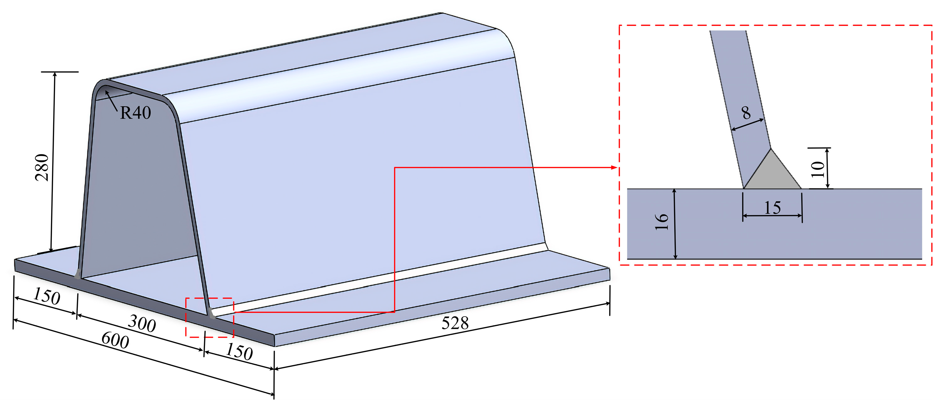
2.2. Sample and Welding Process

According to the typical structural details of an actual bridge, the RTD joints used in the welding experiment were consistent with those in real bridges. The dimensions of the bridge deck and the U-rib are shown in Figure 1. In order to reduce the influence of thermal cutting on the test indexes of the experiment, a steel plate and U-rib without any pretreatment and in the as-delivered state were selected as the base metals of the test piece. Firstly, a specimen larger than the actual required size was cut by plasma, and then the heat-affected zone of the specimen was removed by a horizontal band sawing machine. This method uses cold cutting to remove the heat-affected area and avoids the heat effect of plasma cutting on the specimen. The test area of the specimen was polished, and the position of the measuring point was marked before the welding of the specimen. The specimens were precisely welded by the OSD external welding intelligent welding system. This system consists of six advanced welding manipulators and a solid gantry, and has the ability to perform welding operations of multiple U-ribs at the same time. The system design realized the precise control and adjustment of the welding process parameters (including the welding speed, current, voltage, etc.). In addition, the welding system introduced a fully automated control technology, which not only ensured the quality and efficiency of the welding process, but also significantly reduced the labor intensity. In the welding process, the fillet weld ceramic liner is specially used to prevent the leakage welding in the welding, which further improves the integrity and reliability of the welded joint. The welding process is illustrated in Figure 2.

Submerged arc welding was used in the test, and the welding parameters shown in

Table 3. Welding condition.

Welding Technique	Current (A)	Voltage (V)	Welding Speed (mm/s)	Welding Torch Tilt Angle
Submerged arc welding	560~568	34~36	7	30°

were selected. The RTD joint was welded using unilateral full-penetration welding without a groove and with a single-pass weld formation. After the welding was completed, the flux scab on the weld surface and the ceramic liner at the weld root were removed.

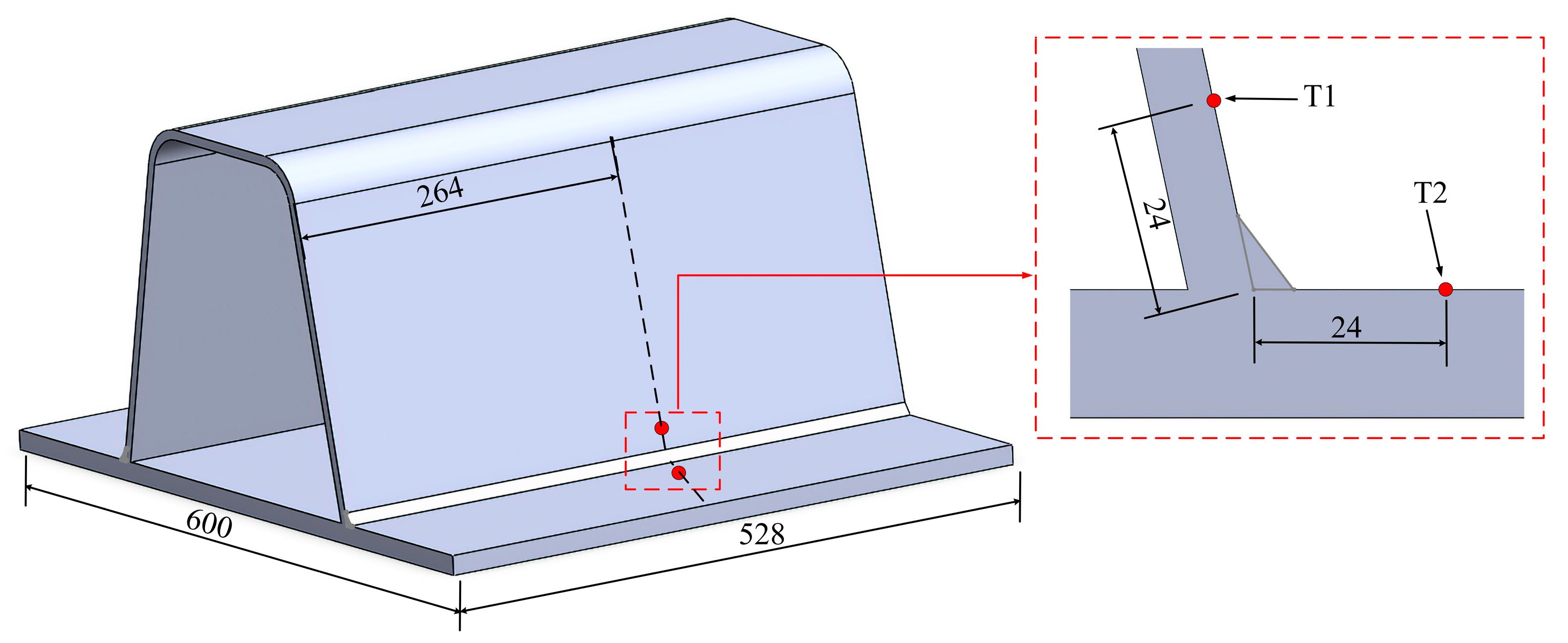
2.3. Temperature Measurement

The YET-640L thermometer and K-type high-temperature thermocouple were used to detect the temperature changes during the welding process, verifying the temperature field obtained from the corresponding finite element model. During welding, as the welding torch advances, the weld bead becomes covered by the melted wire and flux. Thus, the measuring points must not be too close to the weld bead to avoid being covered by the melt and flux, which would make the measuring points ineffective. Two temperature measuring points, T1 and T2, were positioned 24 mm away from the center of the weld, as shown in Figure 3.

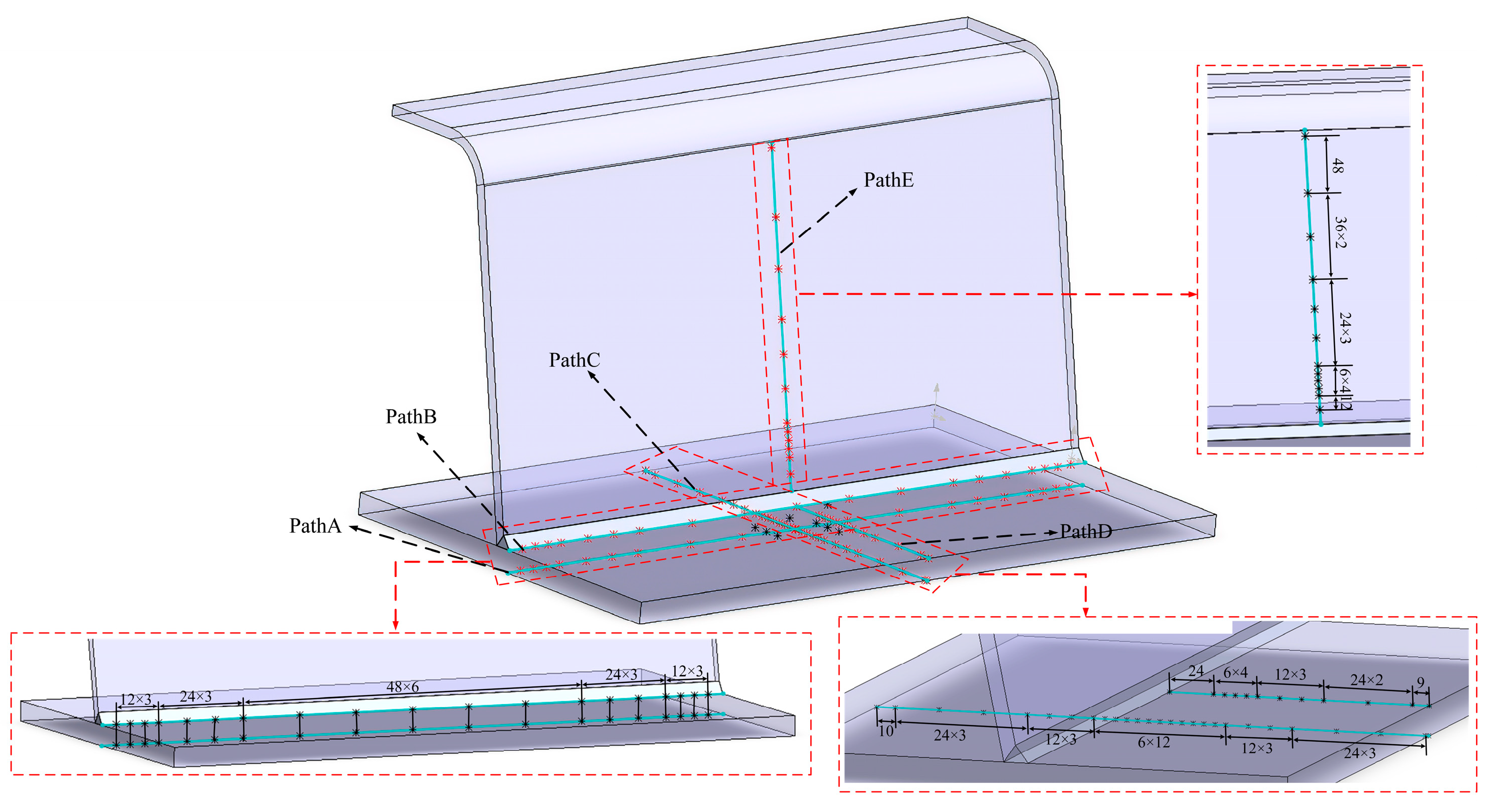
2.4. Stress Measurement

In this test, five test paths were established, including the upper and lower surfaces of the weld (Path A and Path B), the upper and lower surfaces of the roof (Path C and Path D), and the outer surface of the U-rib (Path E). The total number of measuring points was 85. Additionally, the residual stress gradient near the weld area and the arc starting and extinguishing area of the weld was very large. To accurately determine the distribution of the residual stress along the test paths of the specimen, the test points in these areas were properly arranged. The specific positions, arrangement patterns, and distances of the measuring points are shown in Figure 4.

The residual stress was measured by the blind hole method. The blind hole method is a semi-destructive testing method, in which the residual stress of the measured point is released by drilling holes on the surface of the specimen. In the measurement of the residual stress by the blind hole method, it is assumed that there is a general residual stress field in a certain area of an isotropic material. The maximum and minimum principal stresses are σ1 and σ2, respectively. A special strain gage is placed on the surface of the area, and a small hole is made in the center of the strain gage, which causes the stress to release at the edge of the hole, so that the released strain is generated in the area of strain gage removal. According to the released strain measured by the strain gage, the residual stress can be calculated [21]. After the specimen was welded and cooled to room temperature, the residual stress tests were conducted according to the designated measuring points. The YC-III type stress measurement instrument was used to release the residual stress at the measurement point by drilling, and then the magnitude of the released strain in different directions was measured by the strain gage located at the measurement point. Finally, the residual stress calculation formula was used to calculate the residual stress at the measurement point. As shown in Figure 5.

Figure 6 shows the layout of the strain gauge rosettes. After the rosettes were applied, a hole was drilled with the center point at 0. The measured residual stress at each measuring point was applied to the analysis model as the maximum and minimum principal stresses, with the maximum principal stress direction angle β set to 0 in the model before the principal stress was applied (equivalent to the #1 sensitive grating of the strain gauge rosettes being oriented along the direction of the maximum principal stress). Since the test piece was made of isotropic material, and the stress before and after drilling was in the linear elastic stage, the residual principal stress expression (1) could be derived using G. Kirsch’s [22] theory.

$${\sigma }_{\mathrm{1,2}}={\displaystyle \frac{\left({\epsilon }_1+{\epsilon }_3\right)}{4A}}\mp {\displaystyle \frac{1}{4B}}\sqrt{{\left({\epsilon }_1-{\epsilon }_3\right)}^2+{\left({\epsilon }_1+{\epsilon }_3-2{\epsilon }_2\right)}^2}$$

(1)

where ${\epsilon }_1$, ${\epsilon }_2$, and ${\epsilon }_3$ are the strain values of sensitive gates 1, 2, and 3. $A={\displaystyle \frac{\left({\epsilon }_1+{\epsilon }_3\right)}{2\left({\sigma }_1+{\sigma }_2\right)}}$, $B={\displaystyle \frac{\sqrt{{\left({\epsilon }_1-{\epsilon }_3\right)}^2+{\left({\epsilon }_1+{\epsilon }_3-2{\epsilon }_2\right)}^2}}{2\left({\sigma }_2-{\sigma }_1\right)}}$, where $A$ and $B$ are stress release coefficients.

3. Numerical Simulation

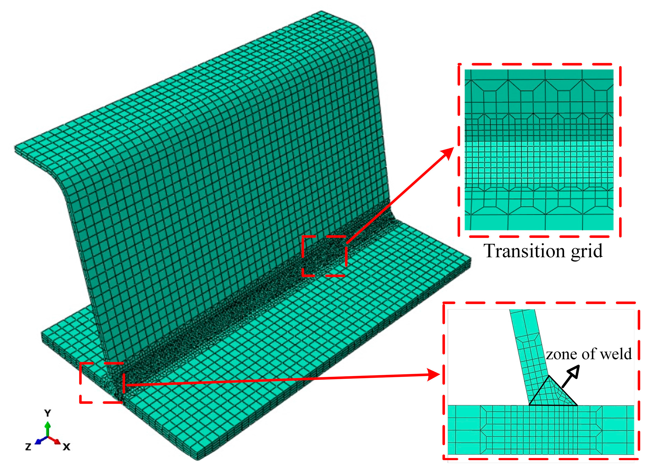
3.1. Finite Element Model

In this study, ABAQUS finite element software was used to establish a numerical model consistent with the size of the test specimen, as shown in Figure 7. To improve the computational efficiency of the finite element model and control the number of model elements, the model was designed based on the symmetry of the actual component. Since the filler material and the base metal had the same strength configuration in this study, the two metals were defined as the same material and given the same Q345qE properties. First, the transient temperature field was determined using thermal elastic–plastic analysis. Subsequently, in the mechanical analysis stage (nonlinear elastic–plastic analysis), the deflection and residual stress of the model were calculated, with the previously determined transient temperature field applied to the model as a thermal load. To further enhance the accuracy of the welding analysis, a fully coupled analysis method was adopted, considering the influence of the phase change latent heat of steel. The analysis model was established by SolidWorks software, and the analysis model was meshed by Hyper Mesh software. When meshing, transition grid technology was used to ensure that the grid in the area near the weld was refined (less than 2 mm), while the grid far from the weld was coarse (more than 12 mm). This method not only ensured the accuracy of the calculation results but also significantly reduced the number of elements, thereby improving the efficiency of the welding analysis. The element type used was an eight-node thermomechanically coupled hexahedral element (C3D8T). Finally, the established finite element analysis model contained 70,771 elements and 61,160 nodes. Through the above methods and model settings, the thermal–mechanical behavior during the welding process could be accurately simulated, effectively improving the computational efficiency and providing reliable data support for the subsequent structural analysis.

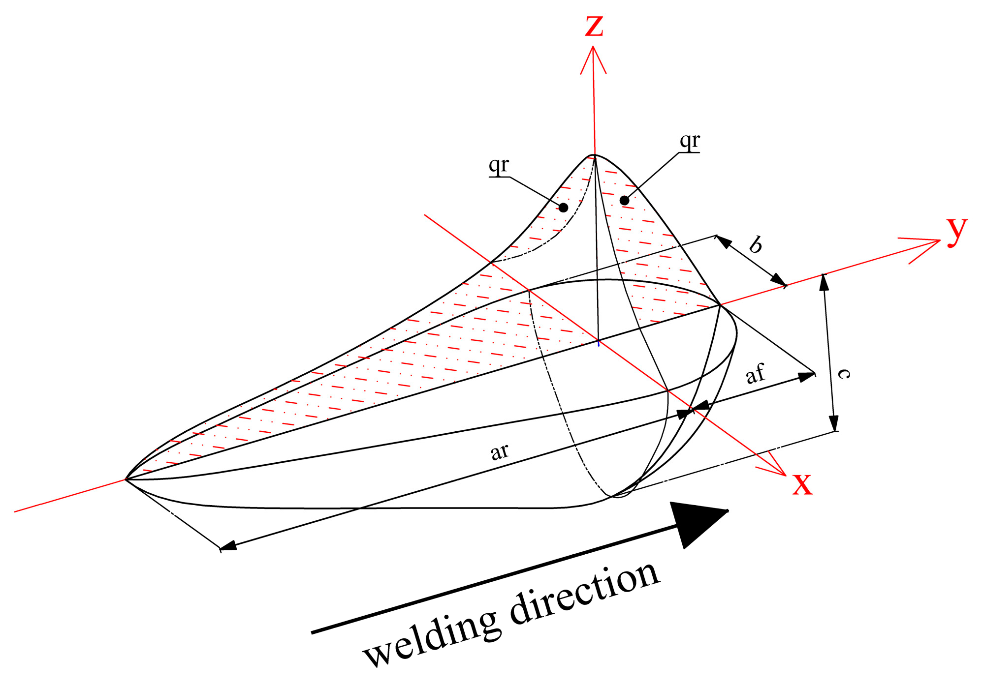
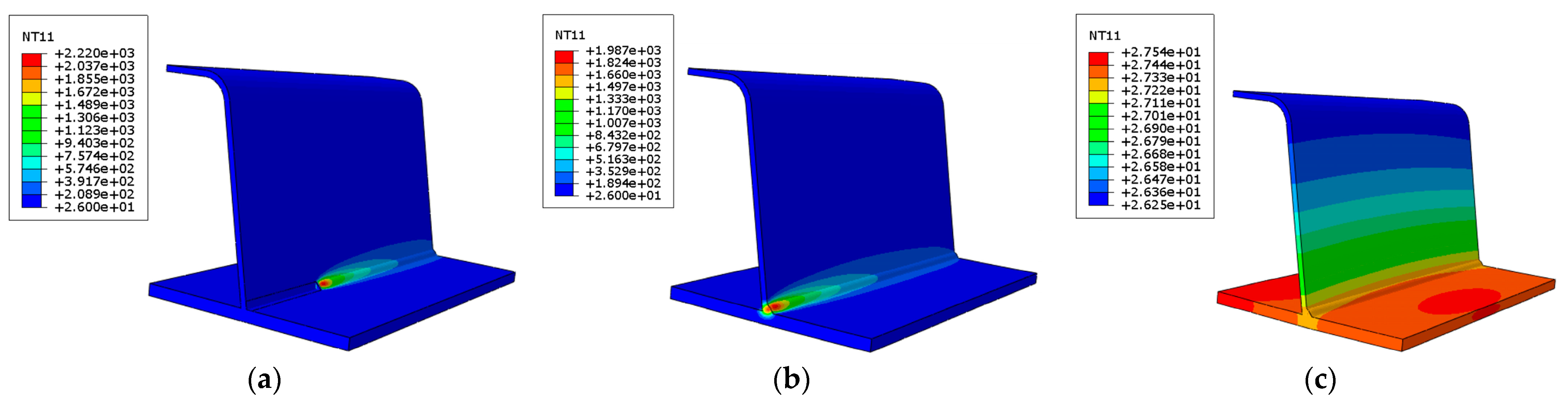
3.2. Heat Source and Thermal Analysis

In the welding analysis process, the load of the model is applied to the weld area in the form of a moving heat source. Common heat sources can be divided into point heat sources, line heat sources, surface heat sources, and body heat sources, depending on their geometric shapes. To simulate the actual welding process more accurately, John Goldak [23] proposed a double ellipsoid heat source model. The heat source distribution function of this model accounts for the large temperature gradient at the front end and the small temperature gradient at the back end during the welding process. Along the welding direction, the welding heat input is divided into two ellipsoids, as shown in Figure 8. In the process of full-penetration welding, the double ellipsoid heat source model more accurately reflects the characteristics of heat source heating along the depth direction. By combining the front and rear ellipsoids, this model can simulate the heat input of the welding heat source at different depths and positions, and more accurately capture the temperature field changes during the welding process. Specifically, the double ellipsoid heat source model describes the heat input distribution of the welding heat source in the front and rear regions of the weld using two ellipsoids. The front ellipsoid describes the heat input at the front end of the welding, where the temperature gradient is large. The rear ellipsoid describes the heat input at the back end of the welding, where the temperature gradient is relatively small. This distribution function design realistically simulates the characteristics of heat source movement during the actual welding process. By using this double ellipsoid heat source model in combination with detailed element meshing, the accuracy of the calculation results can be significantly improved. This method not only enhances the accuracy of welding simulation but also provides reliable theoretical support for optimizing the welding process parameters and improving the welding quality. It is of great significance for studying the thermomechanical coupling effect during welding and its influence on the performance of welded structures.

ABAQUS finite element software cannot directly apply a moving heat source to the analysis model, but ABAQUS analysis software provides a DFLUX subroutine running interface. By combining ABAQUS and Fortran, the heat flux density distribution function and the heat source movement speed are written in Fortran language, which can realize the movement and loading of the welding heat source on the analysis model. For the simulation of the filling process of the weld melt during the welding process, the killing and activation of the weld unit can be realized through the Model Change function provided by the software, that is, the ‘life and death unit method’.

$$q_f={\displaystyle \frac{6\sqrt{3}{f}_{1}Q}{\pi a_{f}bc\sqrt{\pi }}}\mathrm{e}\mathrm{x}\mathrm{p}\left[-3\left({\displaystyle \frac{x^2}{b^2}}+{\displaystyle \frac{y^2}{a_f^2}}+{\displaystyle \frac{z^2}{c^2}}\right)\right]$$

(2)

$$q_r={\displaystyle \frac{6\sqrt{3}{f}_{2}Q}{\pi a_{r}bc\sqrt{\pi }}}exp\left[-3\left({\displaystyle \frac{x^2}{b^2}}+{\displaystyle \frac{y^2}{a_r^2}}+{\displaystyle \frac{z^2}{c^2}}\right)\right]$$

(3)

where Q is the welding power, which can be calculated by Q = $\eta UI$. $\eta$ is the welding efficiency; $U$ [$V$] is the welding voltage; $I$ [$A$] is the welding current; $b$ is the half width of the heat source; $c$ is the depth of the heat source; $a_f$ is the length of the first half of the ellipsoid; $a_r$ is the length of the second half of the ellipsoid; $f_1$ and $f_2$ represent the energy share parameters of the front and rear ellipsoids, respectively.

The double ellipsoid heat source model not only considers the uneven distribution of energy density in the welding heat source but also compensates for the shortcomings of the plane Gaussian heat source model, which cannot account for penetration. It is suitable for welding methods with significant penetration, such as groove welding and fillet welding. It has been widely used in finite element numerical simulations for various welding methods, including electron beam welding, submerged arc welding, and gas-shielded welding [24]. During the welding process, the fluid dynamics and thermal processes in the weld pool, the interaction between the base metal and the heat source, and the development of phase change-induced welding stress and strain in the weld metal occur [25].

In order to predict welding residual stress and deformation, the temperature field must be accurately determined, necessitating the calibration of the heat source model. By adjusting the heat source parameters, the nodal temperatures captured by the thermocouples in experimental measurements should be closely matched with the corresponding nodal temperatures obtained from the simulation, thereby calibrating the heat source. Further calibration is completed by matching the boundaries of the weld pool in the finite element model with the weld pool macrograph of the tested weld section. The selection of appropriate parameters for the heat source model is crucial for the accuracy and efficiency of the calculation. The heat source parameters and their values adjusted for thermal analysis are shown in

Table 4. Adjusted heat source parameters.

Parameter	$\mathit{b}$	${\mathit{a}}_{\mathit{f}}$	${\mathit{a}}_{\mathit{r}}$	$\mathit{c}$	${\mathit{f}}_1$	${\mathit{f}}_2$
Value	13.8	13.3	43.26	10.64	0.5	1.5

.

The ambient temperature and initial temperature were set to 26 °C during the simulation. The thermal boundary conditions were defined on the outer surface of the geometric model to consider the transfer of convective and radiative heat to the surrounding environment. Fixed-end boundary conditions were applied at the edge to simulate the clamping of the workpiece during the welding process. Thermal boundary conditions are usually used for welding simulation to simulate the heat loss caused by convection and radiation on the free surface of the welded specimen. The distance between the fixture and the heat source was large enough, and the temperature in the clamping area did not rise, so the heat transfer through conduction between the substrate and the fixture was ignored. It was assumed that the sample underwent heat loss by convection and radiation. In this study, this problem was solved by defining a temperature-dependent heat transfer coefficient, which is expressed by the two mathematical expressions of other researchers [26,27], as shown in Equations (4) and (5):

$$h=0.0668\times T\left({\displaystyle \frac{W}{m^2℃}}\right)\hspace{1em}\hspace{1em}0\le T\le 500$$

(4)

$$h=0.231\times T-82.1\left({\displaystyle \frac{W}{m^2℃}}\right)\hspace{1em}\hspace{1em}T\ge 500$$

(5)

where T (°C) is the temperature and h denotes the temperature-dependent heat transfer coefficient.

3.3. Material and Mechanical Analysis

The accuracy of the mechanical and thermal physical parameters of the material directly affects the accuracy of the simulation results. The thermal strain was calculated by the temperature-dependent thermal expansion coefficient. The mechanical properties of the matrix metal and the filler metal required in the structural analysis, that is, the yield strength, Young’s modulus, Poisson’s ratio, and thermal expansion coefficient varying with temperature, were taken from the literature [28]. The more reliable thermal physical and thermodynamic material parameters of Q345qE steel are shown in Figure 9. The numerical simulation of this welding was analyzed and calculated by complete coupling, and the influence of the latent heat of steel phase change was considered. The solid phase temperature of Q345 steel is 1410 °C, the liquid phase temperature is 1515 °C, and the latent heat of solidification is −255.5 J/g [29].

The application of mechanical constraints affects the residual stress field and welding deformation. Considering the actual situation of the welding process, the mechanical boundary conditions were applied in the relevant finite element model to limit the rotation and translation of all nodes in the region. During welding, the fixed fixture pressed the two sides of the specimen panel. In addition to the symmetrical constraints on the symmetrical axis at both ends of the component, simple support constraints and longitudinal constraints along the weld direction were also set. The symmetrical constraint was applied on the symmetrical surface of the U-rib of the bridge deck, the displacement constraint in the Y-axis direction was applied on the two side lines of the roof, and the displacement constraint in the X-axis direction was applied on one side perpendicular to the weld. The X axis was perpendicular to the direction of the weld along the top plate, the Y axis was perpendicular to the direction of the top plate, and the Z axis was along the direction of the weld in order to simulate the effect of the jig and clamping device on the welded specimen in the actual welding process. The equivalent constraint method is shown in Figure 10.

4. Result and Discussion

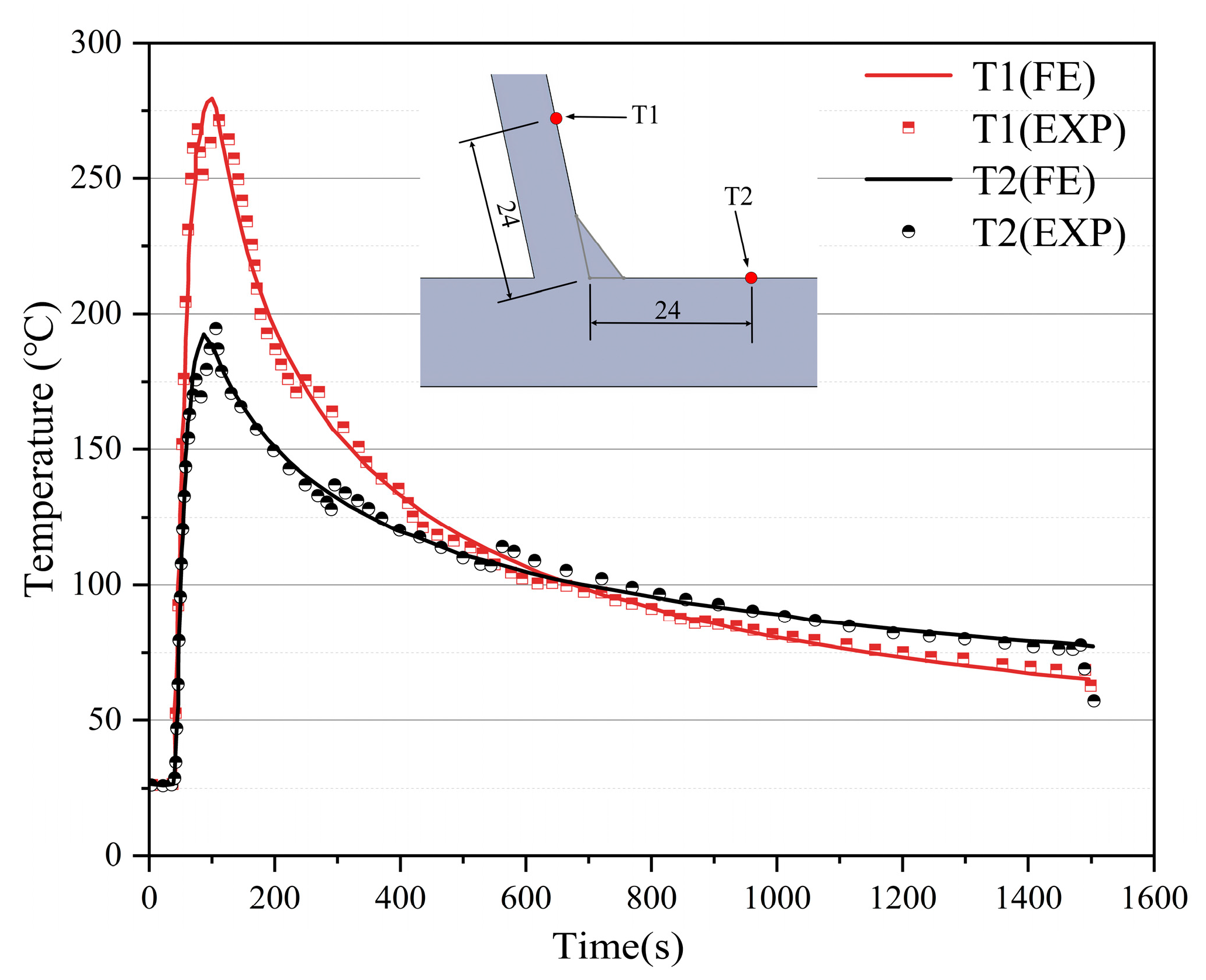
4.1. Temperature Field Results

Figure 11 shows the welding temperature field. The welding temperature field is a dynamic process, influenced by both time and space. As the welding heat source moves, the temperature field distribution on the specimen constantly changes. During welding, the temperature field is primarily concentrated in the weld, with the heat source at the center point, and the temperature field distribution decreases elliptically along the direction opposite to the heat source movement. When the heat source is between the arc starting point and the arc extinguishing point, the temperature at the center of the heat source stabilizes at a maximum value of 2220.30 °C. Once the heat source moves to the arc extinguishing point and the welding ends, the heat source load ceases. At this point, the maximum temperature of the weld decreases to 1987.23 °C and begins to cool, with no incomplete penetration in the arc extinguishing area.

The calibration of the welding temperature field required matching the shape and size of the weld pool of the actual specimen. The weld pool of the specimen was polished and corroded, and the cross-section of the fillet weld in the middle of the specimen (i.e., the penetration depth) was compared with the simulation results. Additionally, the width and length of the molten pool at the end of the welding path were compared with the simulation results. The melting point (1450 °C) of Q345 steel was used as the contour boundary line to extract the molten pool contour of the analysis model, as shown in Figure 12. The weld pool profile obtained from the finite element model closely matched the actual weld pool profile, with a maximum error of only 2.8%, indicating that the real temperature distribution and the heat source model were correctly calibrated.

The node temperatures recorded by the thermocouples are highly consistent with the corresponding node temperatures from the finite element simulation results, which is a primary indicator of accurate temperature distribution and welding thermal cycles. In this study, the temperature variation at specific points on the specimen during the actual welding process was measured using thermocouples. These measurements were then compared and analyzed against the temperature variations at corresponding points in the model. The temperature test results for measurement points 1 and 2 were compared with the node temperatures at the corresponding positions in the welding analysis model. The comparison results are shown in Figure 13.

The temperature results obtained through numerical welding analysis are largely consistent with the actual welding temperatures of the weldment. The temperature at the measurement point 1 rose quickly to its peak and cooled down to a final temperature that was lower than that of measurement point 2. This is because the thickness of the U-rib was approximately half that of the bridge deck. Consequently, the measurement point 1 on the U-rib absorbed and transferred heat faster than measurement point 2 on the bridge deck. However, the actual area of the U-rib that expanded was larger than that of the bridge deck, and the contact surface area available for thermal convection and radiation was also larger. Therefore, measurement point 1 released heat faster than measurement point 2. This analysis confirms that the variation in the temperature field was consistent with the actual situation, proving that the numerical simulation results of the temperature field are accurate and reliable.

4.2. Residual Stress Results

The primary focus of this study was the stress field after welding. Based on the validated finite element model, the transverse and longitudinal residual stresses of each component were numerically analyzed. To verify the structural analysis results, the residual stress after welding was measured, as shown in Figure 14.

The maximum equivalent residual stress after welding was 448.34 MPa. The longitudinal residual tensile stress of the roof was the highest in the weld zone, and the residual tensile stress decreased while the compressive stress increased as the distance from the weld increased. The area farthest from the weld in the vertical direction also experienced significant compressive stress due to constraints. The distribution of transverse residual stress on the roof surface differed from that of the longitudinal residual stress, with the maximum tensile stress occurring in the arcing section corresponding to the weld. During the cooling process, the initial welding part of the arc starting section in the weld center restricted the transverse shrinkage of the subsequent welding part, leading to transverse compressive stress. This created an equilibrium state along the plate thickness, resulting in substantial tensile stress at this position on the roof surface.

To calibrate the finite element model, the release strain of all measuring points along five test paths of a single-sided full-penetration welding RTD joint was tested. The size characteristics and variation rules of transverse residual stress and longitudinal residual stress in each path were obtained and compared with the numerical analysis results. The accuracy and reliability of the stress field in the finite element (FE) model of single-sided full-penetration welding were verified by the experiment (EXP). The measured results of the simulated transverse residual stress (TRS) and longitudinal residual stress (LRS) along the five test paths—Path A, Path B, Path C, Path D, and Path E—are shown in Figure 15.

The residual stress values obtained by numerical analysis were generally consistent with the experimental values. The residual stress on the upper surface of the weld (Path A) and the lower surface of the weld (Path B) along the welding direction was primarily transverse compressive stress in the arc starting and arc extinguishing areas, while longitudinal tensile stress was predominant in the central stable area. The maximum tensile stress was 407.46 MPa, and the maximum compressive stress was −378.62 MPa. Due to the high residual stress, the weld toe and the connection between the U-rib and the top plate were prone to cracking and structural fatigue. The heat-affected zone had a large thermal gradient, resulting in a significant stress gradient, particularly in the direction perpendicular to the weld. The stress in the vertical direction of the weld shows a large gradient with increasing distance from the weld. The residual stress on the upper surface of the top plate (Path C) and the lower surface of the top plate (Path D) perpendicular to the welding direction was mainly longitudinal residual stress. There was a small compressive stress on both sides of the weld, with an average value of about −95 MPa, and a large tensile stress in the area approximately 25 mm around the weld, with a maximum value of 380.87 MPa. The stress gradient in this area was significant. The residual stress on the outer surface of the U-rib (Path E) was primarily longitudinal residual stress, with tensile stress within 38 mm from the weld root, reaching a maximum value of 334.09 MPa. The area farther from the weld exhibited mainly small compressive stress, which decreased with increasing distance.

After the processing and production of OSDs, they need to be put into practical engineering to bear long-term wheel load, and the weld root and weld toe are prone to fatigue damage. Under the action of repeated stress amplitude, fatigue failure mainly occurs in the weld area. The fatigue life of this area is shorter than that of other areas. Among them, the weld toe is the easiest and the first to occur fatigue failure. Farther away from the weld, the degree of fatigue failure becomes smaller and smaller. Therefore, the size characteristics and distribution of residual stress are very important for the study of fatigue life.

4.3. Influence of Welding Parameters

4.3.1. Roof Panel Thickness

The influence of welding residual stress on fatigue performance varies with different plate thicknesses [30,31]. Figure 16 shows the WRS distribution and size on the outer surface of the U-rib (Path E) and the upper surface of the roof (Path C) under different plate thicknesses (12 mm, 14 mm, and 16 mm). For residual stress on the weld surface, the residual tensile stress gradually decreased with increasing plate thickness. In the arc starting section, the maximum difference was about 20 MPa, while in the stable area, the difference was small, around ±10 MPa. On the outer surface of the rib, residual stress gradually transitioned from tensile to compressive as the distance from the weld increased, and both tensile and compressive stresses decreased with increasing plate thickness. On the upper surface of the roof, the tensile stress at the weld decreased as roof thickness increased. A thicker roof results in a smaller tensile stress range, which is related to the reduction in the heat-affected zone with increasing roof thickness during the actual welding process.

4.3.2. Welding Speed

The welding speed mainly affects the magnitude of residual stress after welding by influencing the welding temperature field [32]. When the heat input per unit of time is constant, the welding line energy is closely related to the welding speed, which affects the energy absorbed by the weldment. Given the reasonable matching of other welding parameters, it was necessary to study how welding speed changes the stress field by affecting the temperature field. Figure 17 compares the WRS distribution and size on the outer surface of the U-rib (Path E) and the upper surface of the roof (Path C) under different welding speeds (7.5 mm/s, 9 mm/s, and 10.5 mm/s). On the upper surface of the roof, although the peak stress did not change significantly with increasing welding speed, the overall residual stress decreased, and the tensile stress boundary area also decreased, though the change was small. The compressive stress on the surface of the U-rib decreased with increasing welding speed. The maximum longitudinal residual tensile stress also decreased with increasing welding speed, but the effect was minimal, within ±10 MPa. This may have been due to a small welding speed gradient or the selection of a load step size in the finite element calculation.

5. Conclusions

The WRS distribution of single-sided full-penetration welded RTD joints was studied by means of an experiment and numerical simulation. According to the experimental measurement and analysis, the main conclusions and observation results are summarized as follows:

(1)

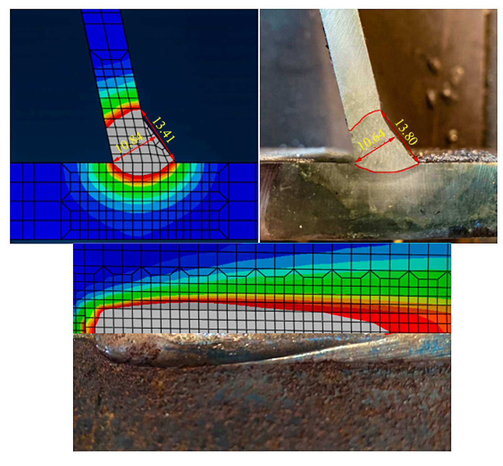
Through the combination of simulation and experimental methods, the single-sided full-penetration welding effect of OSDs under specific welding process conditions was systematically explored. Under the experimental conditions, the welding current was set to 564 A, the welding voltage was 35 V, and the welding speed was 7 mm/s. The single-pass weld forming without a groove was successfully realized, and the weld penetration rate was ensured to meet the technical requirements of more than 100%. This finding provides an efficient and economical solution for the welding process of orthotropic steel bridge decks.

(2)

The FE results are in good agreement with the EXP measurement results, indicating the accuracy of the FE model. In the vicinity of the weld, the longitudinal WRS was significantly higher than the transverse WRS, revealing the anisotropy of stress distribution during welding. The peak value of the residual tensile stress appeared near the weld. With the increase in distance, the stress gradually decreased along the vertical weld direction and transformed into compressive stress. In the stress distribution of the weld surface, the maximum tensile stress was 407.46 MPa, and the maximum compressive stress was −378.62 MPa. The average residual stress on the surface of the plate was about−95 MPa, indicating the dominant role of compressive stress. However, in the area of about 25 mm on both sides of the weld, the tensile stress increased significantly, and the maximum value reached 380.87 MPa. This phenomenon is of great significance for evaluating the fatigue performance of the welded structure. For the outer surface of the U-rib, the residual stress was mainly longitudinal. In the range of 38 mm from the root of the weld, the stress was mainly tensile stress, and the maximum recorded value was 334.09 MPa. This finding further emphasizes the influence of the welding details on the overall structural performance.

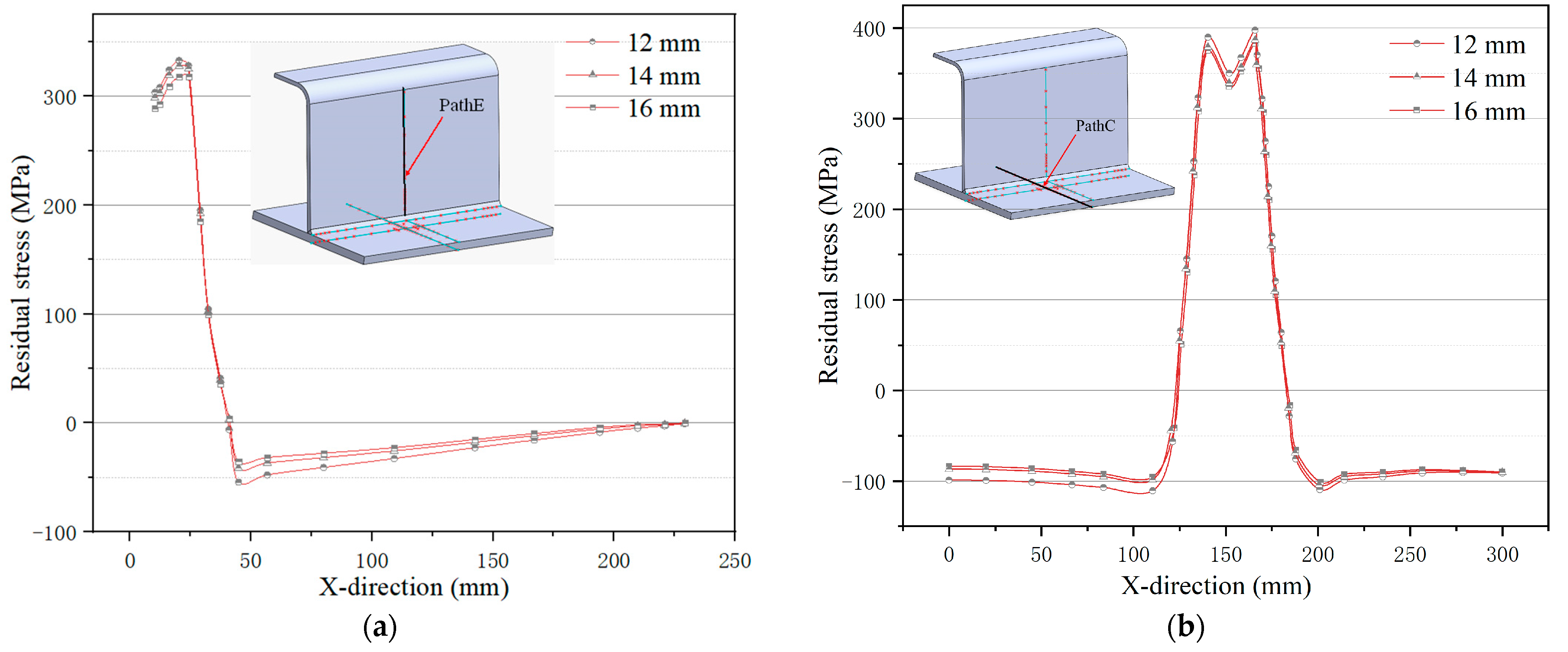
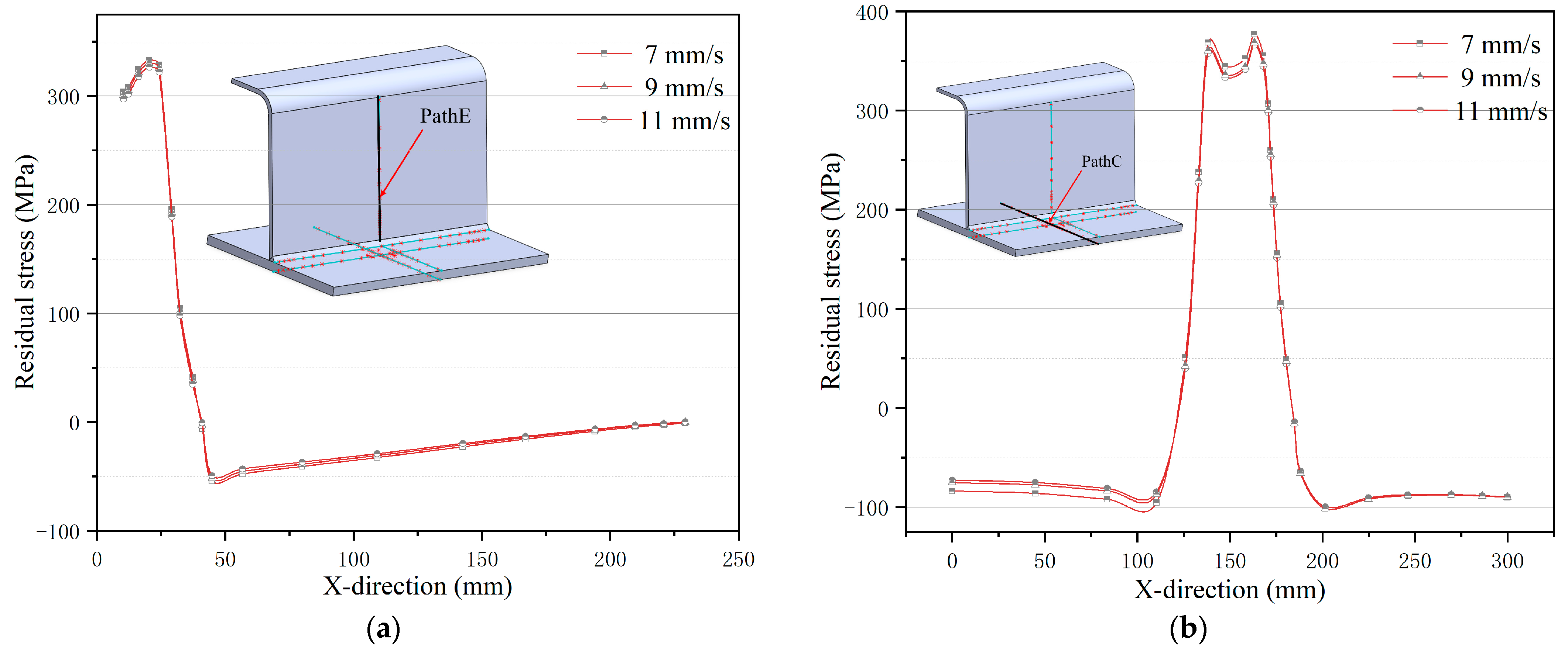
(3)

Based on the results of FE analysis, the effects of roof thickness and welding speed on WRS were discussed. The longitudinal stress of the RTD joint decreased with the increase in the welding speed, which indicates that the welding speed is an important factor affecting the residual stress. At the same time, the increase in the roof thickness also led to a decrease in the longitudinal residual stress, although the effect was relatively small. For the WRS of the top plate and the outer surface of the U-shaped rib, it was found that the influence of the thickness of the top plate and the welding speed was not significant, indicating that these parameters have limited influence on the residual stress distribution characteristics in a specific area.

In this paper, only single-sided full-penetration welding under a specific welding process was studied, and the influence of different welding processes was not studied. In the analysis, only half of the RTD joint was used as the analysis model for welding simulation. At the same time, the effects of secondary factors, such as stirring, convection, chemical reaction, and creep and phase transformation of the materials in the molten pool were ignored. In the future, the above problems can be studied in more depth.

References

1. Zhang, Q.; Ma, Y.; Cui, C.; Chai, X.Y.; Han, S.H. Experimental investigation and numerical simulation on welding residual stress of innovative double-side welded rib-to-deck joints of orthotropic steel decks. J. Constr. Steel Res. 2021, 179, 106544. [Google Scholar] [CrossRef]
2. Abdelbaset, H.; Cheng, B.; Tian, L.; Li, H.T.; Zhang, Q.H. Reduce hot spot stresses in welded connections of orthotropic steel bridge decks by using UHPC layer: Experimental and numerical investigation. Eng. Struct. 2020, 220, 110988. [Google Scholar] [CrossRef]
3. Cheng, Z.; Zhang, Q.; Bao, Y.; Deng, P.; Wei, C.; Li, M. Flexural behavior of corrugated steel-UHPC composite bridge decks. Eng. Struct. 2021, 246, 113066. [Google Scholar] [CrossRef]
4. Wang, S.; Pei, J.; Ren, F.; Qin, S.; Li, Z.; Xu, G.; Wang, X. Numerical study of full penetration single-and double-sided U-rib welding in orthotropic bridge decks. Case Stud. Constr. Mater. 2024, 20, e03120. [Google Scholar] [CrossRef]
5. Maddox, S.J. Fatigue Strength of Welded Structures; Woodhead Publishing: Sawston, UK, 2014. [Google Scholar]
6. Maljaars, J.; Pijpers, R.; Wu, W.; Kolstein, H. Fatigue resistance of rib to deck, crossbeam to deck and deck to deck welds in orthotropic decks using structural stress. Int. J. Fatigue 2023, 175, 107742. [Google Scholar] [CrossRef]
7. Martucci, D.; Civera, M.; Surace, C. Bridge monitoring: Application of the extreme function theory for damage detection on the I-40 case study. Eng. Struct. 2023, 279, 115573. [Google Scholar] [CrossRef]
8. Civera, M.; Sibille, L.; Fragonara, L.Z.; Ceravolo, R. A DBSCAN-based automated operational modal analysis algorithm for bridge monitoring. Measurement 2023, 208, 112451. [Google Scholar] [CrossRef]
9. Ueda, Y.; Yamakawa, T. Analysis of thermal elastic-plastic stress and strain during welding by finite element method. Jpn. Weld. Soc. Trans. 1971, 2, 116–123. [Google Scholar] [CrossRef]
10. Cao, B.Y.; Ding, Y.L. Effect of plate thickness on welding residual stress of longitudinal ribs of steel bridge deck. J. Southeast Univ. (Nat. Sci. Ed.) 2016, 46, 565–571. [Google Scholar]
11. Kainuma, S.; Jeong, Y.S.; Yang, M.; Inokuchi, S. Welding residual stress in roots between deck plate and U-rib in orthotropic steel decks. Measurement 2016, 92, 475–482. [Google Scholar] [CrossRef]
12. Ji, B.H.; Li, K.K.; Fu, Z. Welding residual stress analysis of steel bridge deck roof and U rib joint. J. Jiangnan Univ. (Nat. Sci. Ed.) 2015, 14, 197–201. [Google Scholar]
13. Lee, C.H.; Chang, K.H. Numerical analysis of residual stresses in welds of similar or dissimilar steel weldments under superimposed tensile loads. Comput. Mater. Sci. 2007, 40, 548–556. [Google Scholar] [CrossRef]
14. Perić, M.; Garašić, I.; Tonković, Z.; Vuherer, T.; Nižetić, S.; Dedić-Jandrek, H. Numerical prediction and experimental validation of temperature and residual stress distributions in buried-arc welded thick plates. Int. J. Energy Res. 2019, 43, 3590–3600. [Google Scholar] [CrossRef]
15. Mathar, J. Determination of initial stresses by measuring the deformations around drilled holes. Trans. Am. Soc. Mech. Eng. 1934, 56, 249–254. [Google Scholar] [CrossRef]
16. Kang, L. Numerical Simulation of Welding Residual Stress of Longitudinal and Transverse Ribs of Orthotropic Steel Bridge Deck; Southwest Jiaotong University: Chengdu, China, 2015. [Google Scholar]
17. Kung, C.L.; Lin, A.D.; Huang, P.W.; Hsu, C.M. Estimation formula for residual stress from the blind-hole drilling method. Adv. Mech. Eng. 2018, 10, 1687814018787409. [Google Scholar] [CrossRef]
18. Van Puymbroeck, E.; Nagy, W.; De Backer, H. Influence of the welding process on the residual welding stresses in an orthotropic steel bridge deck. Procedia Struct. Integr. 2018, 13, 920–925. [Google Scholar] [CrossRef]
19. Lee, C.K.; Chiew, S.P.; Jiang, J. Residual stress study of welded high strength steel thin-walled plate-to-plate joints part 2: Numerical modeling. Thin Walled Struct. 2012, 59, 120–131. [Google Scholar] [CrossRef]
20. Sterling, D.; Sterling, T.; Zhang, Y.; Chen, H. Welding parameter optimization based on Gaussian process regression Bayesian optimization algorithm. In Proceedings of the 2015 IEEE International Conference on Automation Science and Engineering (CASE), Gothenburg, Sweden, 24–28 August 2015; pp. 1490–1496. [Google Scholar] [CrossRef]
21. Chen, X.R.; Zhao, Z.Y.; Jiang, Y.Y. Experimental study on welding residual stress of box section with over-limit width-thickness ratio. J. Civ. Eng. 2010, 43, 281–285. [Google Scholar]
22. Lurie, A.I. Theory of Elasticity; Springer Science & Business Media: Berlin/Heidelberg, Germany, 2010. [Google Scholar]
23. Goldak, J.; Chakravarti, A.; Bibby, M. A new finite element model for welding heat sources. Metall. Mater. Trans. B 1984, 15, 299–305. [Google Scholar] [CrossRef]
24. Kalita, K.; Burande, D.; Ghadai, R.K.; Chakraborty, S. Finite element modelling, predictive modelling and optimization of metal inert gas, tungsten inert gas and friction stir welding processes: A comprehensive review. Arch. Comput. Methods Eng. 2023, 30, 271–299. [Google Scholar] [CrossRef]
25. Yang, W.; Shi, Y.; Wang, Y.; Shi, G. Three-dimensional finite element analysis of welding residual stress of structural steel. J. Jilin Univ. 2007, 3, 347–352. [Google Scholar]
26. Yaghi, A.; Hyde, T.H.; Becker, A.A.; Sun, W.; Williams, J.A. Residual stress simulation in thin and thick-walled stainless steel pipe welds including pipe diameter effects. Int. J. Press. Vessels Pip. 2006, 83, 864–874. [Google Scholar] [CrossRef]
27. Shankar Goud, B.; Dharmaiah, G. Role of Joule heating and activation energy on MHD heat and mass transfer flow in the presence of thermal radiation. Numer. Heat Transf. Part B Fundam. 2023, 84, 620–641. [Google Scholar] [CrossRef]
28. Zhou, S.T. Study on Residual Stresses in Full Penetration U-Ribs Stiffened Orthotropic Anisotropic Steel Bridge Panels; Southwest Jiaotong University: Chengdu, China, 2018. [Google Scholar]
29. Huang, L. Study on High Temperature Performance and Stress Analysis of Slab Continuous Casting; Chongqing University: Chongqing, China, 2007. [Google Scholar]
30. Lu, W.L.; Sun, J.L.; Su, H.; Chen, L.J.; Zhou, Y.Z. Experimental research and numerical analysis of welding residual stress of butt welded joint of thick steel plate. Case Stud. Constr. Mater. 2023, 18, e01991. [Google Scholar] [CrossRef]
31. Raftar, H.R.; Ahola, A.; Lipiäinen, K.; Björk, T. Simulation and experiment on residual stress and deflection of cruciform welded joints. J. Constr. Steel Res. 2023, 208, 108023. [Google Scholar] [CrossRef]
32. Wang, M.; Ning, F.; Pei, Y.; Wang, Y.; Cao, J.; Zhao, L.; Xu, Q.; Zhu, Z. A novel Aluminium-stabilized Stacked REBCO Tape Cable. IEEE Trans. Appl. Supercond. 2024, 34, 4802509. [Google Scholar] [CrossRef]
Figure 1. The shape and size of the specimen (unit: mm).
Buildings 14 02641 g001
Figure 2. Welding process of specimen.
Buildings 14 02641 g002
Figure 3. Arrangement of temperature measuring points (unit: mm).
Buildings 14 02641 g003
Figure 4. Layout of residual stress measuring points (unit: mm).
Buildings 14 02641 g004
Figure 5. Blind hole perforation measurement.
Buildings 14 02641 g005
Figure 6. Distribution states of equivalent stresses.
Buildings 14 02641 g006
Figure 7. Finite element model and meshing.
Buildings 14 02641 g007
Figure 8. Welding heat source model.
Buildings 14 02641 g008
Figure 9. Mechanical and thermophysical parameters of materials. (a) Thermophysical properties of Q345qE steel; (b) plastic stress–strain curve of Q345qE steel.
Buildings 14 02641 g009
Figure 10. Application of model displacement beam.
Buildings 14 02641 g010
Figure 11. Welding temperature field (unit: °C). (a) Welding at 37.71 s (intermediate point). (b) Welding at 75.43 s (arc extinguishing point). (c) Cooling 3600 s after welding.
Buildings 14 02641 g011
Figure 12. Comparison of shape and contour of molten pool (unit: mm).
Buildings 14 02641 g012
Figure 13. Comparison of numerical simulation results and experimental test results of temperature measurement points.
Buildings 14 02641 g013
Figure 14. The plastic stress distribution of the specimen after complete cooling (unit: MPa).
Buildings 14 02641 g014
Figure 15. Equivalent residual stresses on different paths. (a) Path A and Path B transverse residual stress. (b) Path A and Path B longitudinal residual stress. (c) Path C and Path D transverse residual stress. (d) Path C and Path D longitudinal residual stress. (e) Path E longitudinal residual stress and transverse residual stress.
Buildings 14 02641 g015
Figure 16. Longitudinal residual stress under different plate thicknesses. (a) Path E longitudinal residual stress distribution. (b) Path C longitudinal residual stress distribution.
Buildings 14 02641 g016
Figure 17. Longitudinal residual stress at different welding speeds. (a) Path E longitudinal residual stress distribution. (b) Path C longitudinal residual stress distribution.
Buildings 14 02641 g017