Wind-Induced Aerodynamic Responses of Triangular High-Rise Buildings with Varying Cross-Section Areas

Abstract

This study investigated the aerodynamic behavior and structural responses of prismatic and tapered high-rise buildings under extreme wind conditions, focusing on peak wind-induced forces and moments. Using Computational Fluid Dynamics (CFD) simulations with a hybrid RANS/LES approach, the analysis explored the effects of turbulent inflow on the mean pressure coefficients, vortex dynamics, and force coefficients at different wind incidence angles (0°, 30°, and 60°). The results revealed significant differences in peak aerodynamic loads between prismatic and tapered building shapes. The tapered models experienced larger vortex formations and greater suction effects, particularly at two-thirds of the building height, with peak across-wind forces occurring at a 30° wind incidence angle. In contrast, the prismatic model showed the highest peak in along-wind forces and base overturning moments at a 60° wind incidence angle, with Karman vortex shedding and horseshoe vortices prominently captured. The study also highlighted the importance of unsteady inflow conditions in accurately predicting peak dynamic responses, particularly in the wake flow, where vortices significantly influence aerodynamic loads.

1. Introduction

In urban areas characterized by densely packed high-rise buildings strategically designed to optimize land use, the shape of the structures becomes a critical factor when considering the impact of wind forces on the buildings. Beyond this functional requirement, over time, the construction of taller and more imposing buildings has enhanced cities’ cultural and economic profile, showcasing technological prowess. The effect of wind load action is relatively insignificant on low and heavy buildings, where vertical loading prevails. However, as buildings evolve into high-rise structures characterized by lightweight and slender designs, wind loading becomes crucial in the structural design process. The significance of wind loading has increased due to advancements in high-strength materials and rigid, lightweight structural elements. These developments allow for the design and construction of progressively more slender high-rise buildings. In the dynamic response of high-rise buildings, Mattias et al. (2023) conducted a study investigating the response of an H-shaped building to wind loading compared to simplified section buildings. Computational Fluid Dynamics (CFD) and a novel methodology were employed to analyze wind load, which was validated against wind tunnel data. The study delved into the along-wind responses to different wind speeds and dynamic reactions to various wind directions. The findings indicated that, despite experiencing smaller responses in two directions, the H-shaped building displayed larger displacements under specific wind loads when compared to an equivalent rectangular building [1].

Honerkamp et al. (2022) investigated the impact of turbulence in tornadic wind flows, emphasizing the crucial role of accurate turbulence modeling in numerical simulations. The study compared two turbulence modeling approaches (LES with a Smagorinsky–Lilly subgrid and the k-ω model) in simulating real-world tornadoes and their interaction with structures. The focus was on understanding how turbulence model selection influences the simulated tornadic wind flow and induced pressure on surfaces, particularly in the presence of buildings. The analysis compared velocity, pressure fields, and pressure distributions on building surfaces across different turbulence modeling cases [2]. Germi et al. (2021) conducted Computational Fluid Dynamics (CFD) simulations using a large eddy simulation (LES) turbulence model to evaluate the interference effects of two CAARC standard tall buildings. They were concerned with turbulent wind flow of changing Reynolds numbers [3]. Mahdi et al. (2021) explored the accuracy of the Rayleigh damping model, incorporating an explicit operator, in evaluating the dynamic response of high-rise buildings subjected to seismic loads [4]. Chauhan et al. (2022) studied the impact of interfering buildings on the wind pressure distribution around a primary tall rectangular building. To determine how wind loads and pressures are affected by height changes, the interfering building placement was allowed to move horizontally. In contrast, its relative height above the primary one varied [5].

It is widely recognized that various factors impact the behavior of high-rise buildings under wind loads. Some key factors include the height, plan aspect ratio, slenderness ratio, damping, and structure geometry. Generally, building design codes provide provisions and recommendations for calculating wind load on structures with regular and symmetrical cross-section shapes [6]. This study presents an economically efficient numerical approach to introduce wind-induced dynamic forces and vibrations to a triangular full-scale high-rise building model (depicted in Figure 1) under unsteady flows. Subsequently, the resulting aerodynamic forces were repeatedly employed to conduct structural dynamics analyses using Fluid–Structure Computational simulations that involved Fluid–Structure Interactions (FSIs), which require the flow equations to be solved multiple times in conjunction with structural dynamics computations. Due to this, a significant amount of computational time is dedicated to solving flow equations [7].

The calculation of aerodynamic forces was accomplished through a sophisticated combination of different techniques, including an advanced inflow turbulence generator, the computationally efficient Spalart–Allmaras DES turbulence modeling approach, and a conventional FSI load transfer system. The dynamic displacement of the model was analyzed using structure analysis, which assumed linear elastic material behavior and independent mode shapes. The study also considered the effects of aeroelasticity by incorporating aerodynamic damping functions. The importance of turbulent inflow conditions and aerodynamic damping is discussed in detail [8].

Table 1. Summary of recent literature.

Ref.	Short Description
[12]	This experimental study was carried out to determine the “optimal” aerodynamic force coefficients by applying the probabilistic method on tall buildings.
[13]	The purpose of this study was to investigate the effect of interference between two C-shaped high-rise buildings using computational fluid dynamics.
[1]	This study was carried out to determine the dynamic behavior of H-shape tall buildings subjected to wind loading using stochastic and CFD methodologies.
[14]	In this study, rigid modeling and aeroelastic model tests of a proposed steel super-high-rise building with a height of 838 m and a facade that changes along the height were carried out in two typical wind fields.
[15]	This paper proposed a computational approach for aerodynamic shape optimization of a high-rise rectangular building with wings.
[16]	This study aimed to assess the aerodynamic behavior of supertall buildings with three-fold rotational symmetric plan shapes.
[17]	This study computed the wind-induced response of corner modified ‘U’-shaped tall buildings.
[18]	This study examined the wind-induced vibration and dynamic response of a pentagonal high-rise building model.
[19]	This paper evaluated CFD turbulence models that simulated the external airflow around different building roofs using wind tunnel experiments.
[20]	This study was carried out to determine the wind-induced vibrations of high-rise buildings using unsteady CFD and modal analyses.
[21]	This study determined the aerodynamic forces and wind pressures acting on square-plan tall building models with various configurations: corner cut, setbacks, helical, and so on.

presents a summary of prior studies conducted on aerodynamic wind design [9,10,11].

Table 1 provides an overview of the previous research on high-rise buildings, highlighting a range of geometric configurations, including prismatic, C-shaped, H-shaped, and other complex forms. These studies have significantly contributed to our understanding of the aerodynamic behavior and wind-induced responses associated with various building shapes. However, most of the existing research primarily addressed non-tapered or slightly modified structures, leaving a gap in the comprehensive analysis of how tapered geometries influence aerodynamic performance, especially under varying wind angles such as 0°, 30°, and 60°. The aerodynamic response of buildings with tapered shapes, particularly in relation to the wind direction and angle of incidence, remains underexplored. This study sought to address this gap by systematically investigating the effects of different tapering geometries on aerodynamic performance by analyzing the impact of tapering on wind loads and structural stability, especially under critical wind angles.

Several researchers emphasized the significance of geometry in assessing wind loads and investigating their dynamic impacts. Tanaka et al. (2012) conducted wind tunnel experiments to determine the aerodynamic forces and wind pressures exerted on models of tall buildings with square plans and different configurations [21]. Zhou et al. (2021) delved into the aerodynamic features of towering buildings, particularly those with corner alterations. In a separate study [22], Assainar et al. (2021) evaluated the effectiveness of aerodynamic modifications implemented on a model with a pentagonal plan. In addition to exploring how alterations in building shapes impact wind load assessment, there has been an emphasis on understanding the behavior of tall buildings subjected to wind loading [18]. Various configurations have been investigated, including L-shaped [23], Y-shaped [24], Z-shaped [25], and E-shaped configurations [26].

Given that regulatory standards typically provide recommendations for regularly shaped buildings and acknowledge the scarcity of information regarding triangular cross-section buildings, the primary aim of this study using this building model becomes essential for a more comprehensive understanding of the aerodynamic behavior and dynamic response of three different models with varying areas with height for wind speeds of 50 m/s at 0°, 30°, and 60° wind incidence angles. The aerodynamic features of the building were analyzed, followed by a dynamic structural analysis using the finite element method. Computational Fluid Dynamics (CFD) was used to calculate the transient wind loads on the model surface and ANSYS Mechanical 2024 R1 was used to determine the model vibrations [27,28,29].

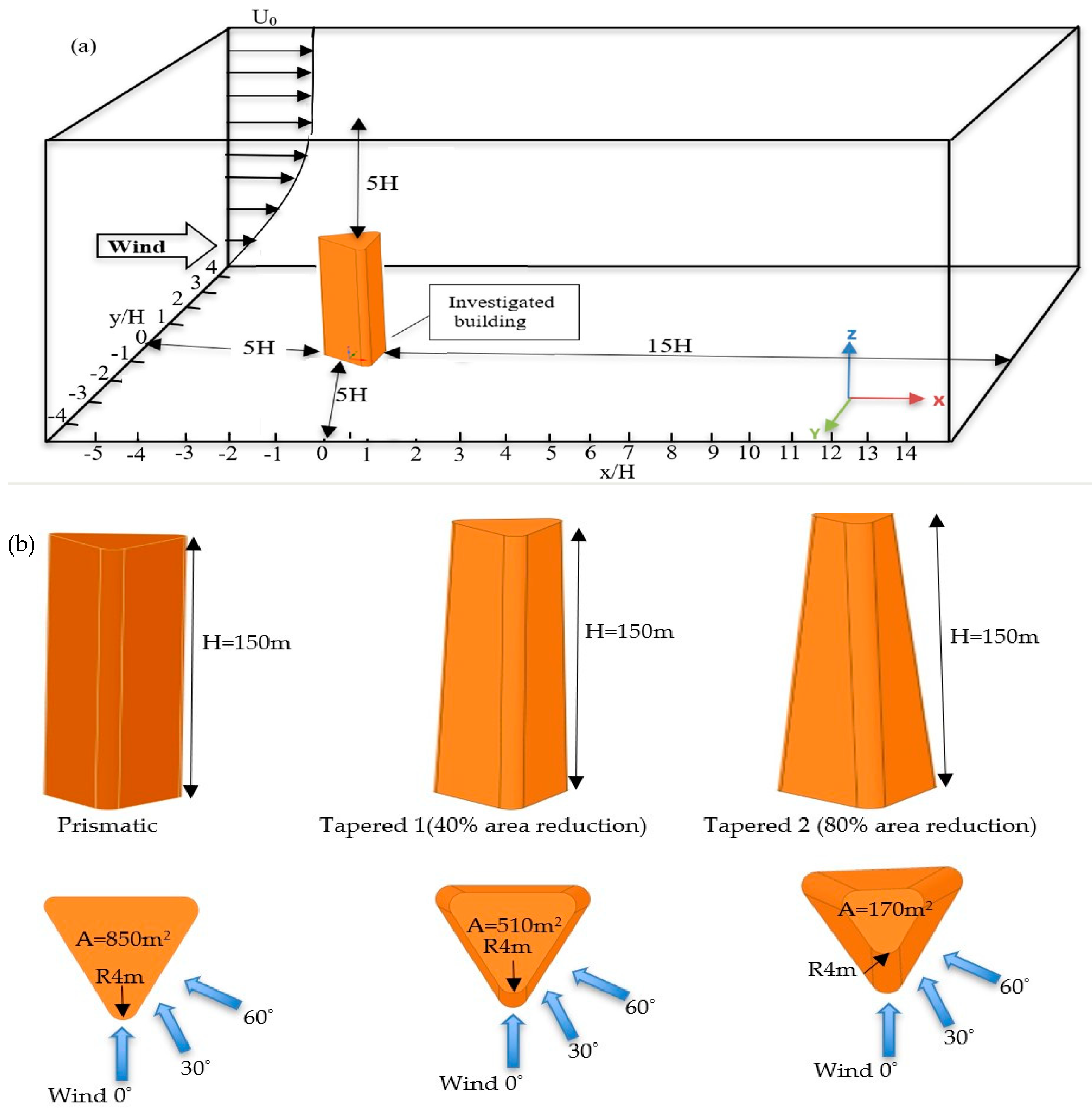
2. Numerical Methodologies

It is crucial to accurately predict the separation and reattachment of air flow when dealing with wind engineering concerning blunt body structures. The turbulence in this study was modeled using a method called the computationally efficient Spalart–Allmaras DES turbulence modeling approach. This combines the use of the Reynolds-averaged NavierStokes (RANS) model and large eddy simulations (LESs) for the near-wall and separated regions, respectively. The Spalart-Allmaras one-equation turbulence model was modified by adjusting the wall distance. The representation of the Spalart-Allmaras unsteady turbulence model is expressed as follows:

$${\displaystyle \frac{\partial \tilde{\nu }}{\partial t}}+u_j{\displaystyle \frac{\partial \tilde{\nu }}{\partial x_j}}={\displaystyle \frac{1}{\sigma \mathrm{R}{e}_{\infty }}}\left\{{\displaystyle \frac{\partial }{\partial x_k}}\left[\left(\nu +\tilde{\nu } \right){\displaystyle \frac{\partial \tilde{\nu }}{\partial x_k}}\right]+{\complement }_{b2}{\displaystyle \frac{\partial \tilde{\nu }}{\partial x_k}}{\displaystyle \frac{\partial \tilde{\nu }}{\partial x_k}}\right\}+{\complement }_{b1}\left(1-f_{t2}\right)\tilde{S}\tilde{\nu }-{\displaystyle \frac{1}{\mathrm{R}{e}_{\infty }}}\left({\complement }_{w1}{f}_w-{\displaystyle \frac{{\complement }_{b1}}{{\kappa }^2}}{f}_{t2}\right){\left({\displaystyle \frac{\tilde{\nu }}{d}}\right)}^2+\mathrm{R}{e}_{\infty }\left(f_{t1}\mathsf{\Delta }{U}^2\right)$$

(1)

The time derivative, convective, diffusion, production, destruction, and source terms are included in the components of the transport equation (Equation (1)). The variable $\tilde{\nu }$ represents a working variable, and the turbulent eddy viscosity, denoted as v_t, is the product of $\tilde{\nu }$ and a near-wall function f_v1, expressed as v_t = f_v1$\tilde{\nu }$. The specifics of the function definitions and closure coefficients are outlined in the original paper [30].

Generally, difficulties associated with standard LES models, especially in near-wall regions, have led to the development of hybrid models aiming to integrate both RANS and LES methodologies within a unified solution strategy. One such example is the Detached-Eddy Simulation (DES) approach introduced in [31]. This model seeks to handle near-wall regions akin to the RANS model while treating the remaining flow in an LES-like fashion. The original formulation involved replacing the distance function ‘d’ in the Spalart–Allmaras (S–A) model with a transformed distance function $\widetilde{d }=\min (d,{\complement }_{DES}{∆}_{max}$), where ‘C’ is a constant and ‘${∆}_{max}$’ signifies the largest dimension of the grid cell under consideration. Although this adjustment to the S–A model is relatively simple, it significantly alters the model’s interpretation. The revised distance function produces a model that behaves as a RANS model in proximity to walls and in a Smagorinsky-like manner away from walls. This is typically justified by influences asserting that the scale dependence of the model becomes local rather than global, a claim supported by dimensional analyses. When the LES component is engaged in the boundary layer, the Detached-Eddy Simulation (DES) model may show inaccurate behavior in thick boundary layers and shallow separation regions. The DES model was implemented using the Spalart–Allmaras turbulence model. The grid was refined near the walls to ensure adequate resolution of the boundary layer, with y-plus values maintained below 1.0. The DES approach effectively transitioned from the RANS model near the walls to LESs in the separated flow regions, allowing for the accurate capturing of large-scale eddies. A second-order upwind scheme was used for convective terms, while a second-order central differencing scheme was applied for diffusive terms to minimize numerical dissipation. When faced with such scenarios, it becomes necessary to increase the precision of the grid at the boundary layer to effectively handle Reynolds stresses [20,32,33]. In turn, it becomes difficult to replace the modeled Reynolds stresses with inadequately resolved Reynolds stresses. This occurrence is known as a modeled stress depletion MSD. In conclusion, reducing stresses helps to decrease skin friction and may result in fragmentation caused by grid restrictions [34,35].

The introduction of unsteady simulated turbulence at the inlet was based on the assumption of homogeneity and isotropy in the turbulent flow. These assumptions, while standard, may introduce certain limitations, particularly in capturing localized flow phenomena. The Spalart–Allmaras DES turbulence model was selected for its ability to accurately simulate separated flows, but it may underpredict the energy in certain turbulent structures. This limitation is acknowledged, and future studies may consider alternative models or refined meshing strategies to address these potential inaccuracies.

2.1. Fluid–Solid Load Transfer

The real-time calculation of a high-rise building’s vibration requires access to the time history of forces that are transmitted to its node elements. Specifically, in this context, wind loads are the external forces that apply flow pressure and shear stresses to the building surfaces. It is essential to accurately transfer these loads from the fluid to the structure [36]. The discretization of the wind flow domain and solid body is distinct due to their unique resolution requirements. The load transfer schemes must demonstrate both numerical accuracy and physical conservatism. The FSI approach in ANSYS 2024 R1 system coupling should transmit the total loads seamlessly from the fluid to the solid, as shown in the flow chart in Figure 2 [37,38].

However, when creating a joint refinement surface, particularly in three-dimensional scenarios, a significant challenge with this scheme was identified. The present study utilized a cautious quadrature-project approach to tackle this problem. This method is simple to incorporate into 3-D simulations and has a relatively minor computational error. Let t_s(x) and t_f(x) represent the traction fields, encompassing pressure and tangential stresses, on the interface boundary Γ between the solid and fluid surfaces. These fields can be estimated by summing up the values multiplied by the corresponding functions [39].

$$t_s(x)\approx {\sum }_{j=1}^{n_s}{N}_s^j(x)t_s^{~j}$$

(2)

$$t_f(x)\approx {\sum }_{j=1}^{n_f}{N}_f^j(x)t_f^{~j}$$

(3)

To minimize the residual of $t_s(x){-t}_f(x)$, the Galerkin weighted residual method was used. This involves multiplying a set of structural shape functions (denoted as W_i = $N_s^i$) and integrating over the surface interface Γ, as expressed below:

$$\iint {}_{\mathsf{\Gamma }}N_s^i\left(x\right) t_s\left(x\right)d\mathsf{\Gamma }=\iint {}_{\mathsf{\Gamma }}N_f^i\left(x\right) t_f(x)d\mathsf{\Gamma }$$

(4)

In the given context, solid surface elements have a shape function, which is represented by $N_s^i\left(x\right)$, and is evaluated at the quadrature points. The traction vector evaluated at these same quadrature points is represented by $t_f\left(x\right)$. A technique to enhance precision is to implement higher order Gaussian integration by adding more points on the surface of the fluid. The current study employed twenty Gaussian points that were evenly distributed over each element of the fluid surface.

In order to obtain high-quality results, the LES model must also have its mesh developed carefully. The grid must be well polished, particularly around the building and in the wake area. As seen in Figure 3, finer meshing has several uses, such as enabling the tracking of flow separation in the building’s steep corners and offering a thorough analysis of vortex-shedding events. When simulating the interaction between the two buildings, the grid quality in the space between them becomes critically important. Using numerical simulations can truly reflect how the complex flow dynamics of interactions between high-rise structures play out. Therefore, the resulting sensitivity to grid resolution is achieved in an all-encompassing way [40].

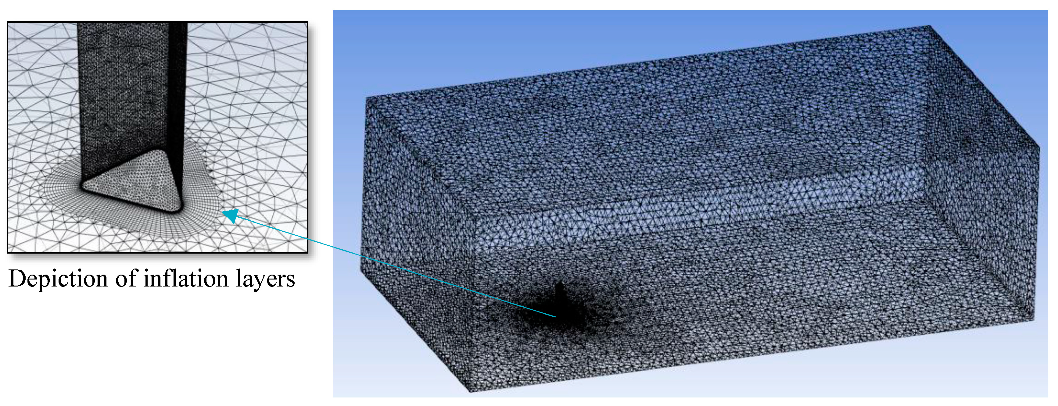
2.2. Mesh Sensitivity Analysis and Estimation of Discretization Error

Mesh sensitivity analysis is an essential step in computational simulations that involves systematically refining the mesh to study how changes in mesh size impact the simulation results. Discretization error estimation, a crucial aspect of this analysis, focuses on the numerical errors introduced when the continuous physical domain is approximated by a discrete mesh.

Step 1 

For three-dimensional calculations, define the representative cell size h as

$$h={⌈{\displaystyle \frac{1}{N}}{\sum }_{i=1}^N(∆V_i)⌉}^{{\displaystyle \frac{1}{3}}}$$

(5)

where $(∆V_i)$ is the volume of the i-th cell and N is the total number of cells used for the computations. Equation (5) should be used when considering integral quantities, such as the drag coefficient. For field variables, the local cell size can be utilized. When an observed global variable is considered, it is appropriate to use an average “global” cell size.

Step 2 

Choose three significantly different sets of grids. For this analysis, use coarse, medium, and fine meshes. Ensure the grid refinement factor

$$\mathrm{r}={\displaystyle \frac{{\mathrm{h}}_{\mathrm{c}\mathrm{o}\mathrm{a}\mathrm{r}\mathrm{s}\mathrm{e}}}{{\mathrm{h}}_{\mathrm{f}\mathrm{i}\mathrm{n}\mathrm{e}}}},$$

(6)

$$r_{21}={\displaystyle \frac{33.28}{16.76}}\approx 1.98$$

$$r_{32}={\displaystyle \frac{16.76}{8.94}}=1.87$$

r = h_coarse/h_fine is greater than 1.3. Run simulations to determine the values of key variables ϕ that are critical to the study.

Let h₁ < h₂ < h₃ and $r_{21}$ = h₂/h₁, $r_{32}$ = h₃/h₂, and calculate the apparent order, p, of the method using the expression

$$p={\displaystyle \frac{1}{\ln \left(r_{21}\right)}}\left|\ln \left|{\epsilon }_{32}/{\epsilon }_{21}\right|+q\left(p\right)\right|$$

(7)

$$q\left(p\right)=\ln \left({\displaystyle \frac{r_{21}^p-s}{r_{32}^p-s}}\right)$$

(8)

$$s=1\cdot sign{\displaystyle \frac{{\epsilon }_{32}}{{\epsilon }_{21}}}$$

(9)

$${\epsilon }_{32}={\varphi }_3-{\varphi }_2$$

(10)

$${\mathsf{\epsilon }}_{32}=-1.40-\left(-1.41\right)=0.01$$

$${\epsilon }_{21}={\varphi }_2-{\varphi }_1$$

(11)

$${\mathsf{\epsilon }}_{21}=-1.41-\left(-1.43\right)=0.02\mathrm{kPa}$$

$$p=0.90$$

Step 3 

Calculate the extrapolated values:

$${\mathsf{\varphi }}_{ext}={\displaystyle \frac{{\mathrm{r}}_{21}^{\mathrm{p}}{\mathsf{\varphi }}_1-{\mathsf{\varphi }}_2}{{\mathrm{r}}_{21}^{\mathrm{p}}-1}}$$

(12)

$${\mathsf{\varphi }}_{ext}=-1.47$$

Step 4 

Calculate and report the error estimates:

Approximate relative error:

$$e_a={\displaystyle \frac{{\varphi }_2-{\varphi }_1}{{\varphi }_1}}$$

(13)

$$e_a=0.00699=1.45\%$$

Extrapolated relative error:

$$e_{ext}={\displaystyle \frac{{\mathsf{\varphi }}_{ext}-{\mathsf{\varphi }}_1}{{\mathsf{\varphi }}_1}}$$

(14)

$$e_{ext}=0.0279=1.38\%$$

Fine grid convergence index (GCI):

$${\mathrm{G}\mathrm{C}\mathrm{I}}_{21,\mathrm{f}\mathrm{i}\mathrm{n}\mathrm{e}}={\displaystyle \frac{1.25{\mathrm{e}}_{\mathrm{a}}}{{\mathrm{r}}_{21}^{\mathrm{p}}-1}}$$

(15)

$${\mathrm{G}\mathrm{C}\mathrm{I}}_{21,\mathrm{f}\mathrm{i}\mathrm{n}\mathrm{e}}=0.0173=1.73\mathrm{\%}$$

Additionally, the error estimates indicate low relative errors and a fine grid convergence index ${\mathrm{G}\mathrm{C}\mathrm{I}}_{21,\mathrm{f}\mathrm{i}\mathrm{n}\mathrm{e}}$ of approximately 1.7261%, suggesting good convergence, as shown in

Table 2. Calculations of discretization error.

Symbol	$\mathbf{\varnothing }$ = Dimensionless Reattachment Length
N1, N2, N3	158,010, 286,730, 564,778
${\mathrm{r}}_{21}$	1.98
${\mathrm{r}}_{32}$	1.87
${\varphi }_1$	−1.43
${\varphi }_2$	−1.41
${\varphi }_3$	−1.40
$p$	0.90
${\varphi }_{ext}$	−1.47
${\mathrm{e}}_{\mathrm{a}}$	1.45%
${\mathrm{e}}_{\mathrm{e}\mathrm{x}\mathrm{t}}$	1.38%
${\mathrm{G}\mathrm{C}\mathrm{I}}_{21,\mathrm{f}\mathrm{i}\mathrm{n}\mathrm{e}}$	1.73%

.

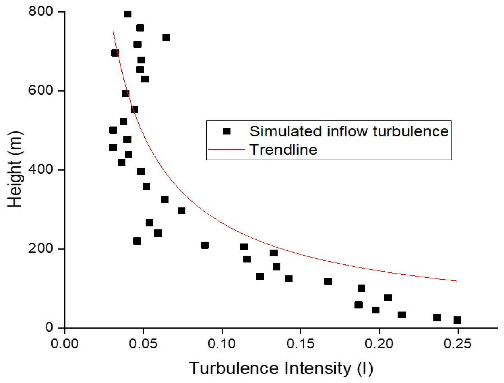
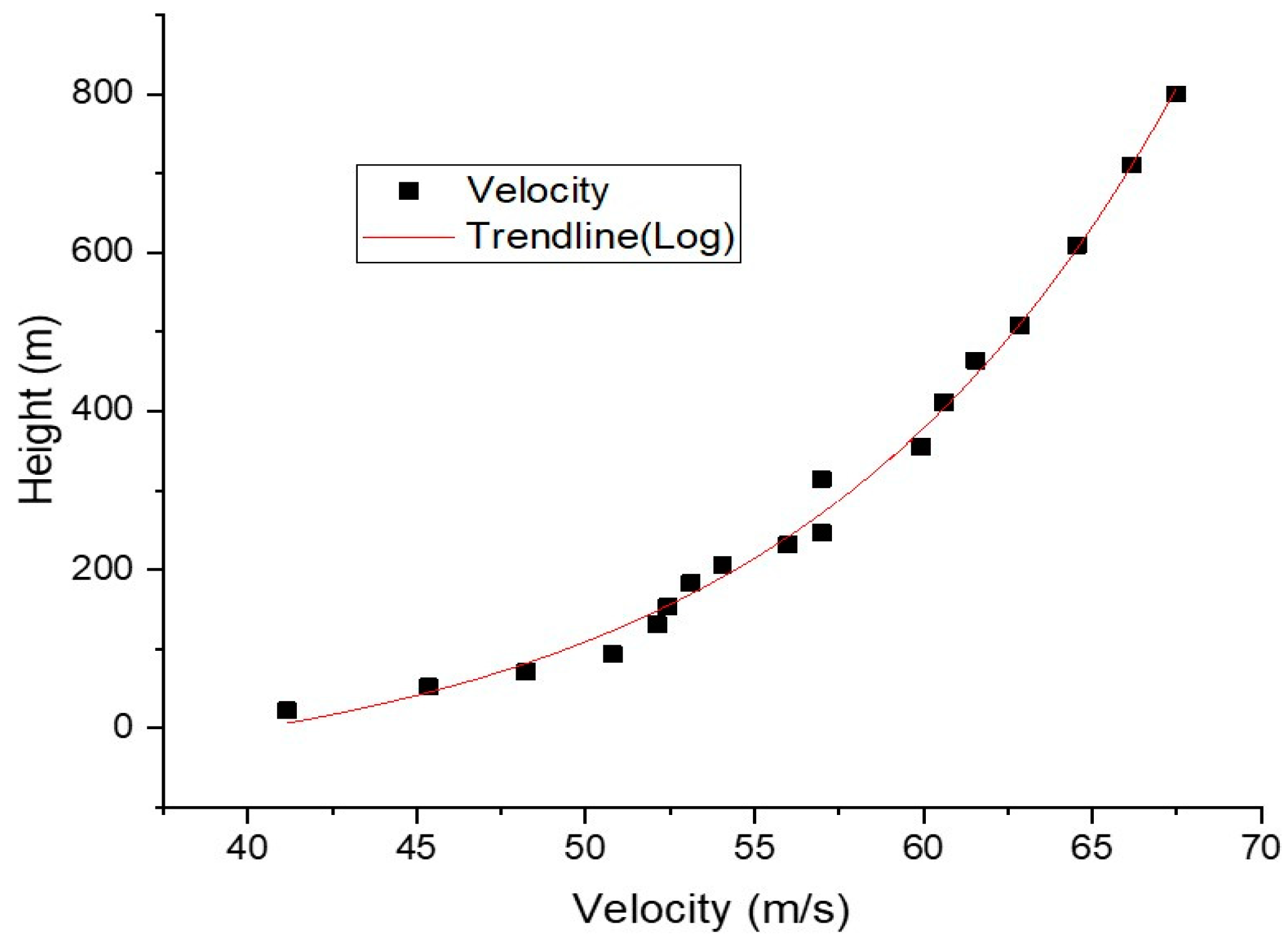
2.3. Turbulence Modeling and Analysis

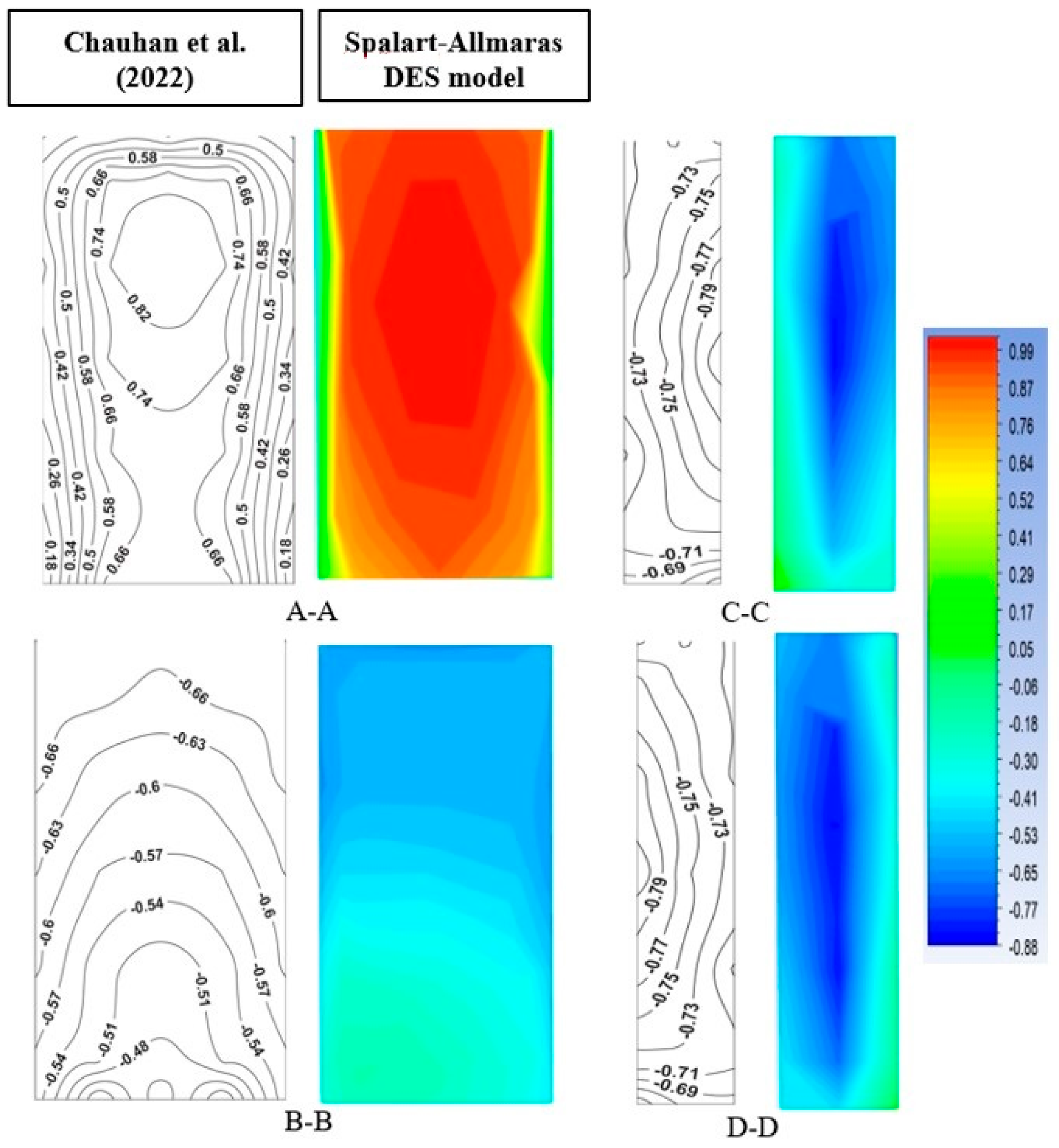
The triangular high−rise building was segmented into smaller parts and presented as two-node frame elements in a three-dimensional format. Each node of these elements has six degrees of freedom, and was created with the assumption of linear elastic behavior of the building material. However, this model does not account for non-linear effects that may result from significant rotations or displacements.

$$\left[M\right]\left\{\ddot{y}(t)\right\}+\left[C\right]\left\{y(t)\right\}=\left\{F(t)\right\}$$

(16)

The given equation involves several key components: the mass matrix denoted as [M], the damping matrix as [C], and the stiffness matrix as [K]. Additionally, it includes the unsteady wind load vector {f(t)}, which was derived from the computational solution, and the displacement vector {y(t)}, which includes translational displacement and rotational angles at each node. It is worth mentioning that the matrices [M], [C], and [K] all have the form (n × n), where n represents the total number of degrees of freedom. It is important to note that, for this particular computation, gravity forces were taken into account [41]. The first stage of the modal analysis requires the representation of the displacement vector {y(t)} in terms of the mode shape matrix [Φ] and the displacement vector {q(t)} in terms of a linear order. This relationship is expressed as follows:

$$\left\{y(t)\right\}=\left[\mathsf{\Phi }\right]\left\{\mathrm{q}\left(\mathrm{t}\right)\right\}$$

(17)

The mode shape matrix [Φ] = [Φ₁, Φ₂, Φ₃,…, Φ_m] is utilized in this computation, where m denotes the total number of mode shapes considered. Matrix [Φ]^T is a transposed matrix multiplied on both sides of the equation; the simplified equation is as follows:

$$\left[\overline{M}\right]\left\{\ddot{q}(t)\right\}+\left[\overline{\complement }\right]\left\{\dot{q}(t)\right\}+\left[\overline{K}\right]\left\{q(t)\right\}=\left\{Q(t)\right\}$$

(18)

with generalized matrices ${\left[\overline{M}\right]=\left[\mathsf{\Phi }\right]}^T\left[M\right]\left[\mathsf{\Phi }\right]$, ${\left[\overline{C}\right]=\left[\mathsf{\Phi }\right]}^T\left[C\right]\left[\mathsf{\Phi }\right]$, and ${\left[\overline{K}\right]=\left[\mathsf{\Phi }\right]}^T\left[K\right]\left[\mathsf{\Phi }\right]$, and a load vector ${\left[Q(t)\right]=\left[\mathsf{\Phi }\right]}^T\{F(t)\}$. A significant characteristic of mode shapes is their linear independence, leading to diagonal matrices. This feature proves highly beneficial, as it streamlines calculations and provides valuable insights into the system’s behavior. As a result, the system under analysis can be separated in the set of ordinary differential equations.

$$\ddot{q_j}+2{\xi }_j{\omega }_j\dot{q_j}+{\omega }_j^2{q}_j=f_j(t),\mathrm{j}=1,2,\dots ,\mathrm{m},$$

(19)

The given expression includes ξ_j, which represents the combined damping due to both structure and aerodynamics, and ω_j = 2πn_j, which indicates the natural angular frequencies of the structure. In mathematical terms, angular frequencies ${\omega }_j^2$ and the mode shape vector $\left\{{\mathsf{\Phi }}_j\right\}$ serve as the eigenvalues and eigenvectors of the system. To determine these values, one can solve the generalized eigenvalue problem involving the matrix $\left[M\right]\left\{{\mathsf{\Phi }}_j\right\}={\omega }_j^2\left[K\right]\left\{{\mathsf{\Phi }}_j\right\}$, with the mass matrix $\left[M\right]$ and stiffness matrix $\left[K\right]$. Ultimately, using Equation (6), one can calculate the time-dependent solution of displacement.

3. Validation

In this study, the absence of access to a wind tunnel laboratory precluded the authors from conducting essential tests. Consequently, we considered a similar model from existing experimental studies performed in [5]. The analysis was conducted using ANSYS CFD 2024 R1 with a methodology similar to that adopted in the current study to authenticate the CFD results. Although a comprehensive comparison of global force coefficients, as undertaken by [5],would be preferable, the limited availability of such data necessitates validation through a comparison of pressure distributions between the experimental and numerical models. The wind tunnel results are juxtaposed with computer simulations to ensure the credibility of the Computational Fluid Dynamics (CFD) modeling methodology and facilitate its applicability to other studies. A model is deemed suitable if the outcomes exhibit similarity [20,42].

It is essential to note that the validation step undertaken in this instance did not utilize the specific building examined in this paper, as the experimental results for that particular structure are unavailable. Instead, the wind tunnel study conducted in [5] was replicated using Computational Fluid Dynamics (CFD) for a building characterized by 60 m × 20 m sides, a height of 160 m, and a rectangular cross-section. The methodology was validated if the results of the wind tunnel experiments and the CFD simulations demonstrate similarity. The authors consistently applied this approach to the simulations and problem-solving, employing turbulence modeling based on the Spalart–Allmaras DES turbulence model, as was used by previous works [20,43,44,45]. Figure 4 displays the results of a wind tunnel experiment [5] and a Computational Fluid Dynamics (CFD) simulation, showcasing the pressure coefficients (Cp). While both studies showed similar pressure patterns across most of the structure, the CFD study revealed an upper-pressure peak that was not present in the wind tunnel investigation. However, as both sets of results exhibited a close correspondence of values and resembled each other in pressure distribution zones, the CFD model was considered suitable for aerodynamic characterization studies of buildings [46].

To validate the simulation results, comparisons were made between available experimental data and the results from other turbulence models. The Spalart–Allmaras DES model was chosen for its balance between computational efficiency and accuracy. The comparison showed that the DES model results showed a good agreement with the experimental data, particularly in capturing peak wind loads and structural responses. The discussion was expanded to highlight the strengths and limitations of the chosen model, offering a more robust validation of the simulation outcomes.

The windward face experienced the highest positive pressure with a peak Cp value of 0.99, while the side walls showed lower values due to flow separation and vortex for-mation. The leeward face experienced negative pressure coefficients, reaching a minimum of approximately −0.88 due to wake formation. A comparative analysis with IS 875 (Part 3)—2015 indicated reasonable agreement show in

Table 3. Comparative analysis of RMS pressure coefficients (Cp).

Face	CFD RMS Cp	IS 875(Part-3)-2015 Cp
A	0.99	0.80
B	−0.40	−0.50
C	−0.88	−0.70
D	−0.40	−0.50

, with the CFD results showing a slightly higher Cp on the windward face (0.99 vs. 0.80) and a more negative Cp on the leeward face (−0.88 vs. −0.70). The side wall values were closely aligned (−0.40 vs. −0.50). The minor deviations observed highlight the enhanced capability of CFD in capturing intricate flow phenomena. This validation demonstrates that CFD simulations provide a credible prediction of pressure coefficients, consistent with IS 875 (Part 3) −2015, thereby reinforcing the use of CFD as a reliable tool for assessing wind loads and informing the design of high-rise buildings.

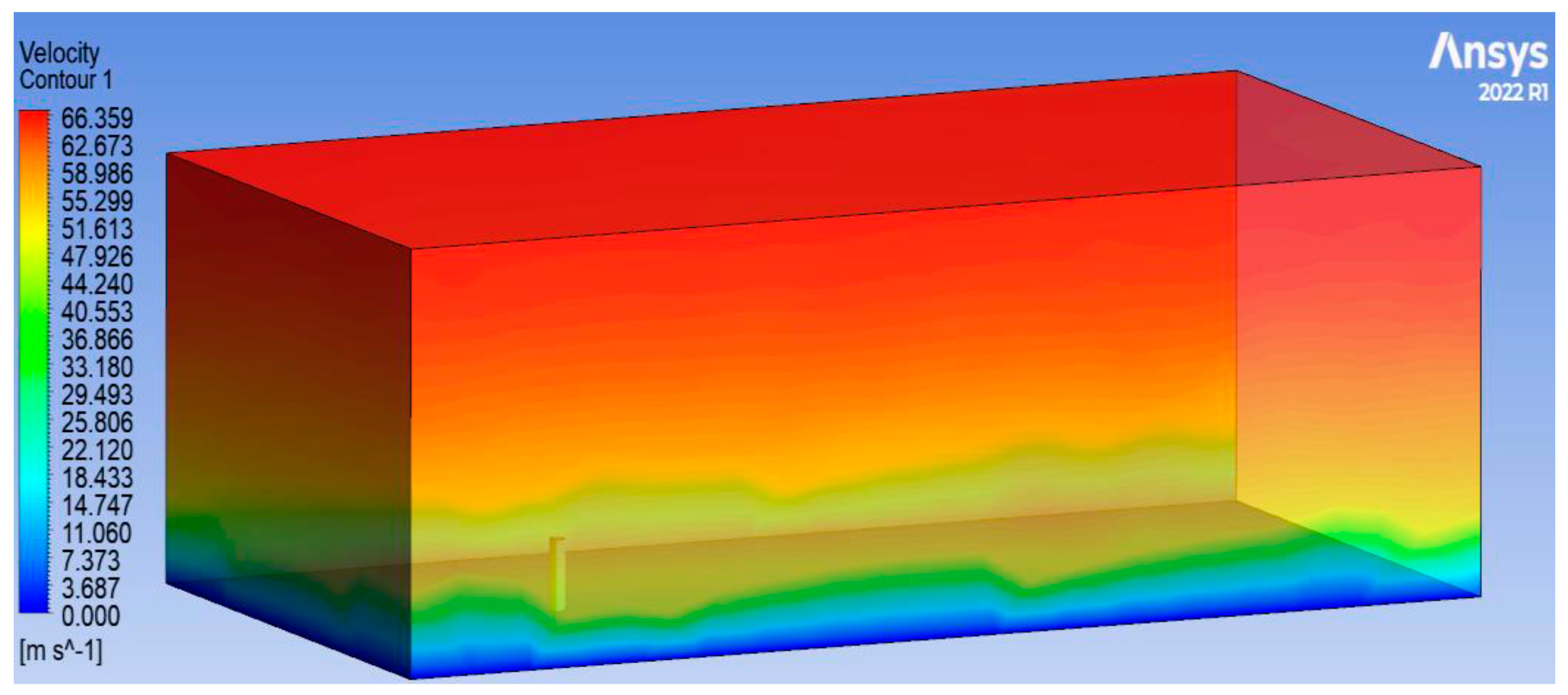
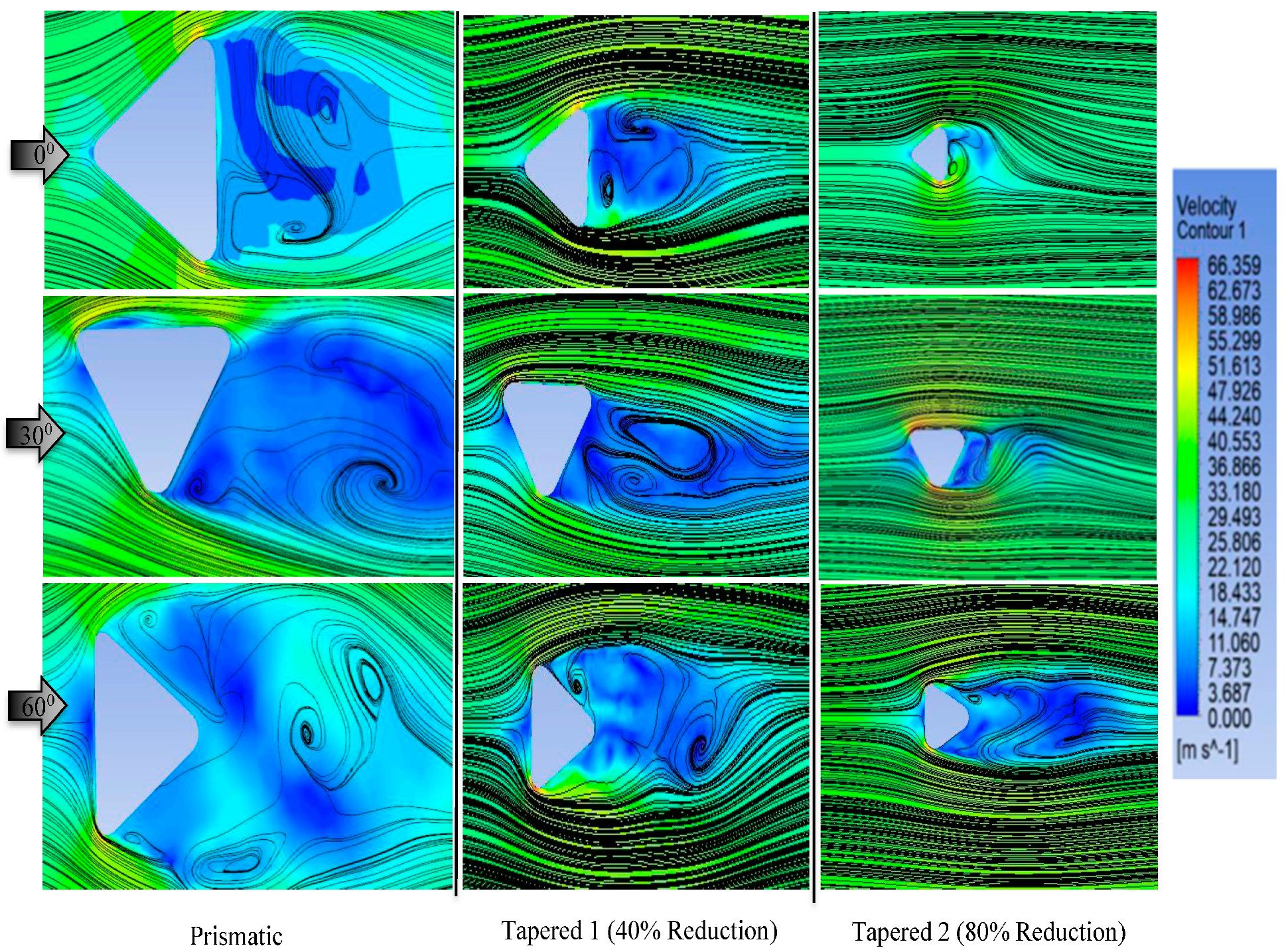
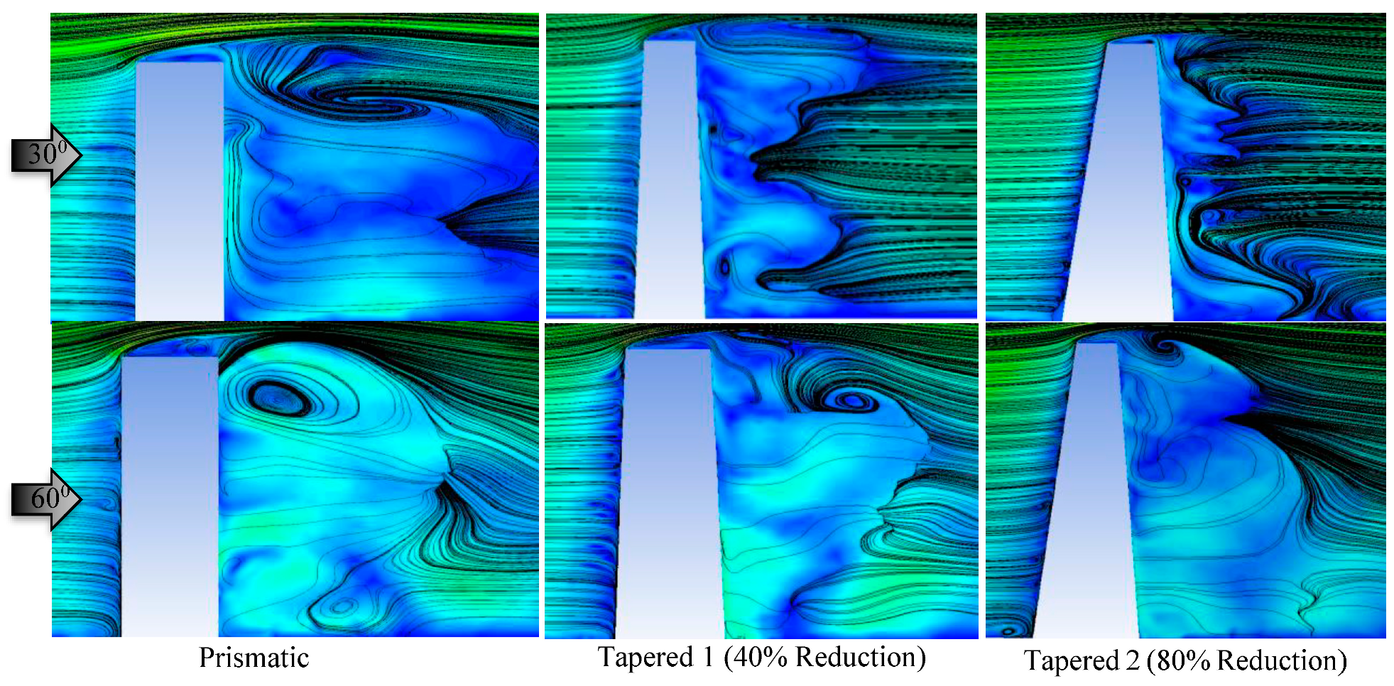
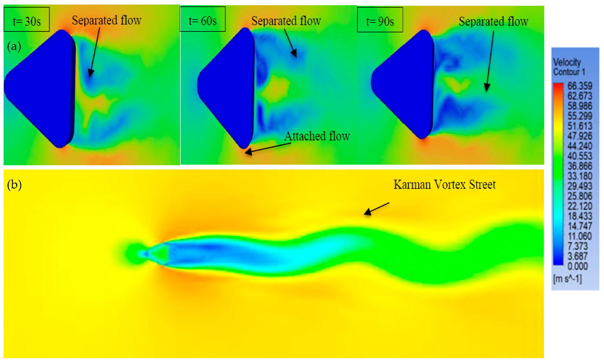
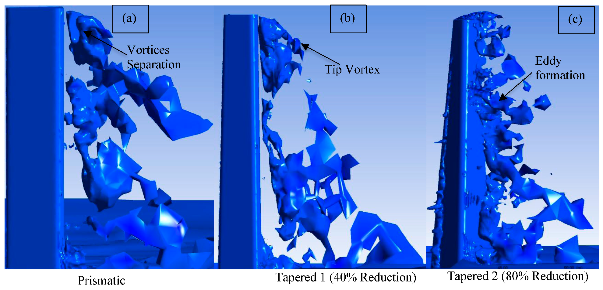
4. Aerodynamic Flow Analysis

Unsteady simulated turbulence was introduced at the inlet of the computational domain. This turbulence is illustrated in Figure 5. The simulated wind displayed temporal variations and replicated key characteristics of natural wind conditions. The velocity profile was defined as U_(z) = U_H(z/H)^α, with U_H = 50 m/s representing the wind speed at the model height, and α is the power-law exponent, which was set to 0.28. The Reynolds number, R = 1.9 × 10⁸, was determined using the model width (B) and velocity (U_H). The turbulence intensity was represented by I_u(Z) = 0.066(z/400)^−0.4 (Figure 6).

$${\mathrm{S}}_{\mathrm{u}}\left(\mathrm{f}\right)={\displaystyle \frac{4{\left({\mathrm{I}}_{\mathrm{u}}{\mathrm{U}}_{\mathrm{a}\mathrm{v}\mathrm{g}}\right)}^2\left(\frac{{\mathrm{L}}_{\mathrm{u}}}{{\mathrm{U}}_{\mathrm{a}\mathrm{v}\mathrm{g}}}\right)}{{\left[1+70.8{\left(\frac{{2\mathrm{f}\mathrm{L}}_{\mathrm{w}}}{{\mathrm{U}}_{\mathrm{a}\mathrm{v}\mathrm{g}}}\right)}^2\right]}^{\frac{5}{6}}}}$$

(20)

$${\mathrm{S}}_{\mathrm{v}}\left(\mathrm{f}\right)={\displaystyle \frac{4{\left({\mathrm{I}}_{\mathrm{v}}{\mathrm{U}}_{\mathrm{a}\mathrm{v}\mathrm{g}}\right)}^2\left(\frac{{\mathrm{L}}_{\mathrm{v}}}{{\mathrm{U}}_{\mathrm{a}\mathrm{v}\mathrm{g}}}\right)\left\{1+188.4\left[2\mathrm{f}{\left(\frac{{\mathrm{L}}_{\mathrm{v}}}{{\mathrm{U}}_{\mathrm{a}\mathrm{v}\mathrm{g}}}\right)}^2\right]\right\}}{{\left[1+70.8{\left(\frac{{2\mathrm{f}\mathrm{L}}_{\mathrm{v}}}{{\mathrm{U}}_{\mathrm{a}\mathrm{v}\mathrm{g}}}\right)}^2\right]}^{\frac{11}{6}}}}$$

(21)

$${\mathrm{S}}_{\mathrm{w}}\left(\mathrm{f}\right)={\displaystyle \frac{4{\left({\mathrm{I}}_{\mathrm{w}}{\mathrm{U}}_{\mathrm{a}\mathrm{v}\mathrm{g}}\right)}^2\left(\frac{{\mathrm{L}}_{\mathrm{w}}}{{\mathrm{U}}_{\mathrm{a}\mathrm{v}\mathrm{g}}}\right)\left\{1+188.4\left[2\mathrm{f}{\left(\frac{{\mathrm{L}}_{\mathrm{w}}}{{\mathrm{U}}_{\mathrm{a}\mathrm{v}\mathrm{g}}}\right)}^2\right]\right\}}{{\left[1+70.8{\left(\frac{{2\mathrm{f}\mathrm{L}}_{\mathrm{w}}}{{\mathrm{U}}_{\mathrm{a}\mathrm{v}\mathrm{g}}}\right)}^2\right]}^{\frac{11}{6}}}}$$

(22)

The integral length scale of turbulence was determined in accordance with the guide-lines provided by the Architectural Institute of Japan [47], which is expressed below:

$${\mathrm{L}}_{\mathrm{u}}={\mathrm{L}}_{\mathrm{v}}={\mathrm{L}}_{\mathrm{w}}=\left\{\begin{array}{c}100, \mathrm{Z}\le 30 \mathrm{m} \\ 100{\left({\displaystyle \frac{\mathrm{z}}{30}}\right)}^{0.5}, 30 \mathrm{m}<\mathrm{z}<600 \end{array}\right.$$

(23)

Accurately modeling inflow turbulence is essential for predicting aerodynamic forces and structural responses with precision. Therefore, it is crucial to carefully examine the characteristics of artificial inflow turbulence. Figure 6 and Figure 7 depict a comparison of the mean velocity and turbulence intensity between numerically generated turbulence and trend profiles. The emphasis was on scrutinizing these two factors. The mean velocity profile had a significant impact on the mean pressure coefficient on the building. The current artificial turbulence demonstrated a mean velocity profile that was almost identical to the target. A gradual increase in observable overshoot towards higher heights was observed, but it had minimal impact on the building model.

5. Results and Discussion

The conducted eigenvalue analysis in this study provided the first ten natural frequencies of the building. Figure 8 presents the corresponding vibration mode shapes and their associated frequency values. The structural assessment involved finite element analysis to ascertain the initial twelve natural vibration frequencies, a crucial requirement for the synthetic wind method employed in this study [19,48]. The first ten natural frequencies of the building in Hertz (Hz) were as follows: 0.28, 0.32, 0.36, 0.79, 1.19, 1.36, 1.79, 2.23, 2.90, and 3.60. The vibration mode shapes illustrated in Figure 8 encompass bending, torsional, and bending–torsional mixed modes [49,50].

Zhang et al. measured and compared the damping ratio and fundamental vibration periods for existing concrete buildings in Korea. They compared these values with those obtained using formulas specified in various codes and research studies.

Table 4. Damping ratios and fundamental vibration periods.

Structural Type	Fundamental Natural Period	Structural Damping Ratio	Ref.
RC Buildings	T = 0.05 H + 0.015 H	2.00%	[51]
RC Buildings	0.0672 H0.75	2%	[52]
RC Buildings	T = 0.022 H = H/46	1.57%	[53]
RC moment frame	Ta = 0.0488 h0.75	2.00%	[54]
RC Buildings	T = 0.0196 H = H/51	0.2467/H + 0.0067	[55]

provides a detailed comparison of the natural vibration periods and damping ratios from different references. It is worth noting that, based on the references in Table 2, the fundamental natural frequency varies with the structural damping ratio [20]. The chosen fundamental natural frequency for the present study was 0.28 Hz, and the adopted damping ratio was 2.00%. The first four frequencies being below 1 Hz imply high flexibility in responding to wind loads, emphasizing the importance of considering the dynamic action of the wind when analyzing the structure’s responses. This underscores the importance of analyzing the structure’s responses while considering the dynamic action of the wind.

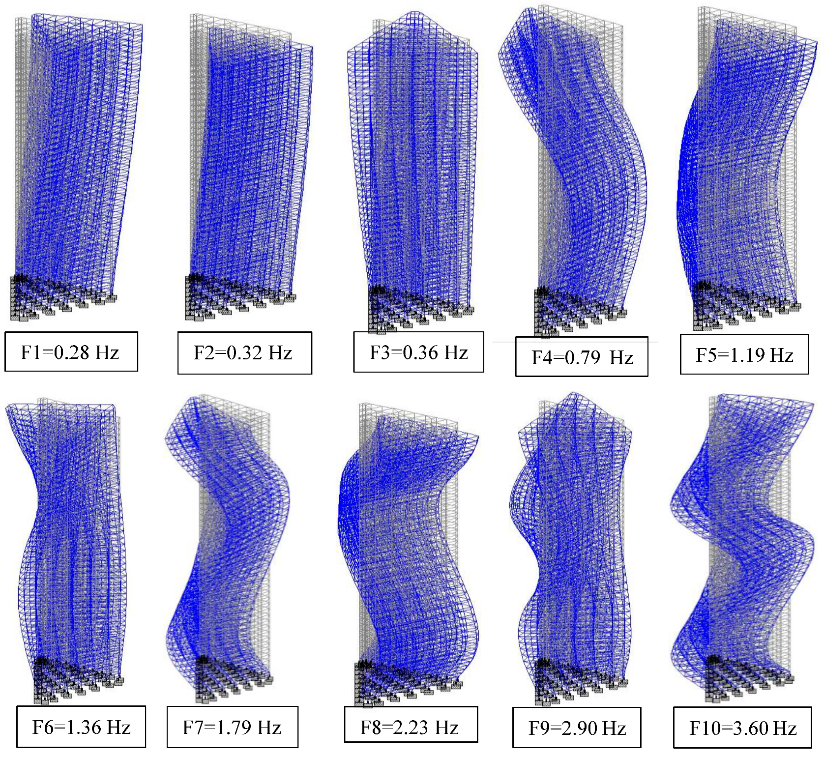
5.1. Dynamic Analyses

The mean pressure coefficient at the building surface is depicted in Figure 9. The increase in unsteadiness with turbulent inflow is apparent. It is worth noting that the pressure coefficient’s is highly dependent on the degree of inflow unsteadiness. Pressure fluctuation variation on the side and back walls was present, but it remained at a low level. When the discretizing and synthesizing random flow generation method is combined with a flow solver, there was a noticeable increase in dynamic pressure fluctuations on the model surface. This increase can lead to general over-prediction. However, since this effect was uniformly applied to all building surfaces, its overall impact on the dynamic responses was minor due to the rigidity of the building. This fact is demonstrated in the following sections.

Figure 10 and Figure 11 illustrate the velocity streamline at horizontal and vertical cross-sections at a height of z = 125 m and with the middle at y = 0, respectively. Notably, large vortices were created at 2/3 the height of the building with a prismatic shape compared to that with a tapered shape, leading to the extensive stretching of mean vortices in the wake flow. The center of the almost symmetric vortices was positioned at 15 m from the building model on the leeward side for the tapered building model. However, this value increased to 20 m from the building for the prismatic building model. In Figure 11, a vortex can be observed near the top and behind the building when moving towards the middle section at y = 0. The vortex at the top decelerated when the simulation used an unsteady inflow, and a much larger vortex was formed with a tapered shape, as shown in Figure 11. The significance of an unsteady flow as the inlet boundary condition was emphasized by observations that accurately predicted the flow field in the vicinity of buildings. In particular, it dramatically affected the wake flow, which generated suction in the across-wind direction and on the leeward side of the building.

Figure 12 illustrates the Karman vortex shedding on the leeward side of the building structure under turbulent inflow conditions. This flow separation around the structure ensured that the flow field behaved similar to real-world conditions. The hybrid RANS/LES modeling captured several crucial features, including the tip vortex over the top of the building, the instantaneous vortices around the model, and the horseshoe vortex at the bottom, as shown in Figure 11. In the wake, these vortices broke up, developed into smaller ones, and ultimately dissipated with flow time due to viscosity [56].

Figure 13 presents the iso-surface of the instantaneous vortical structures for all three models under a 0° wind incidence angle. The Zonal Detached-Eddy Simulation (ZDES) modeling successfully captured critical features like the tip vortex, Karman vortex, and horseshoe vortex. These vortices moved downstream and eventually dissipated due to viscosity effects in the wake. It is worth noting that the tapered building showed larger eddy formation than the prismatic building due to the separation of different velocity streamlines near the wall surface of the building model.

Figure 14a depicts the history of the average across-wind velocity vertex over time. The plot demonstrates that the velocity was constantly fluctuating, indicating that the flow was unsteady. Figure 14b displays the Power Spectral Density (PSD) of the across-wind velocity. This figure highlights an important indicator, which is the frequency corresponding to the peak spectrum. This frequency was found to be about f_uy = 0.0017 Hz.

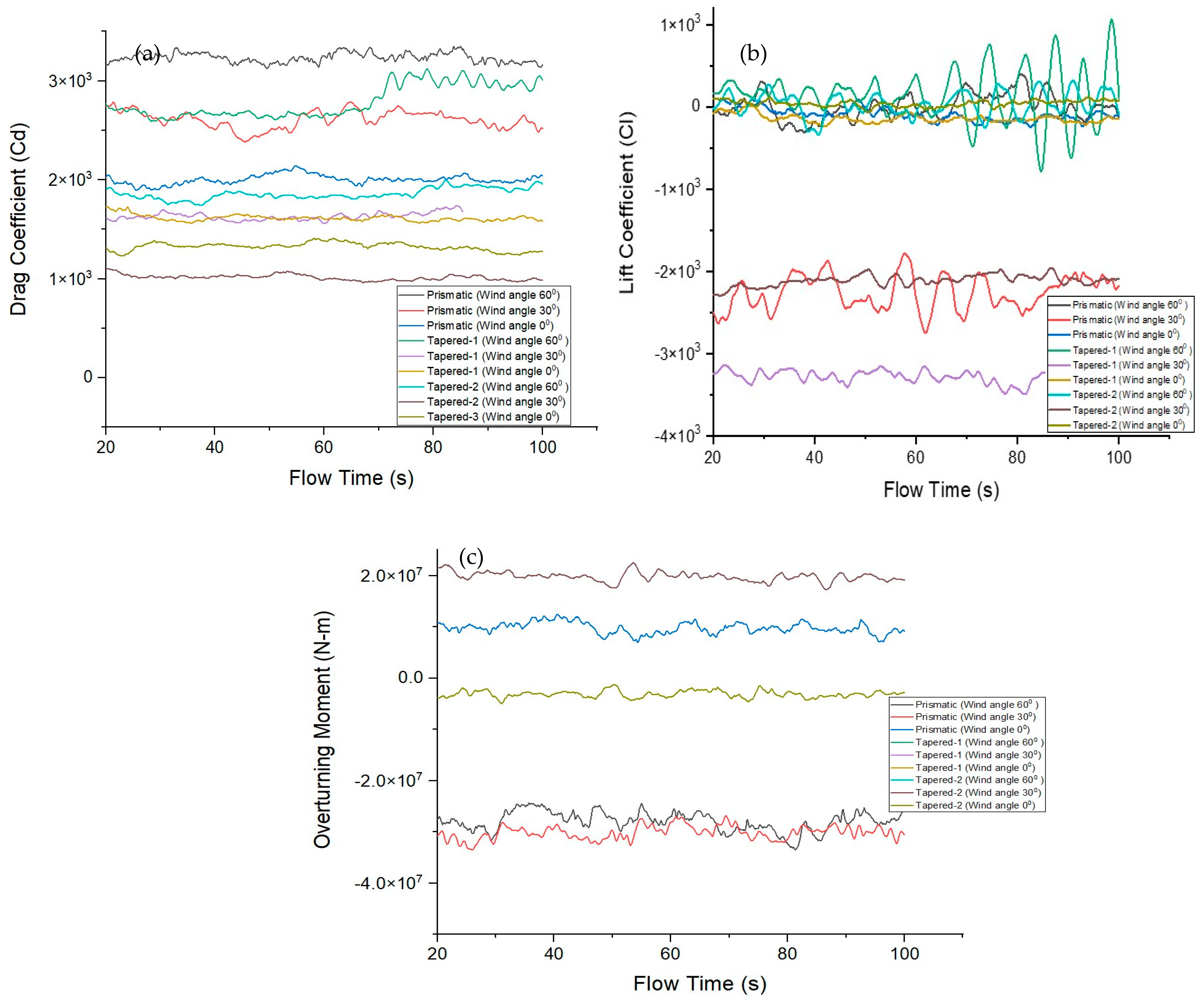
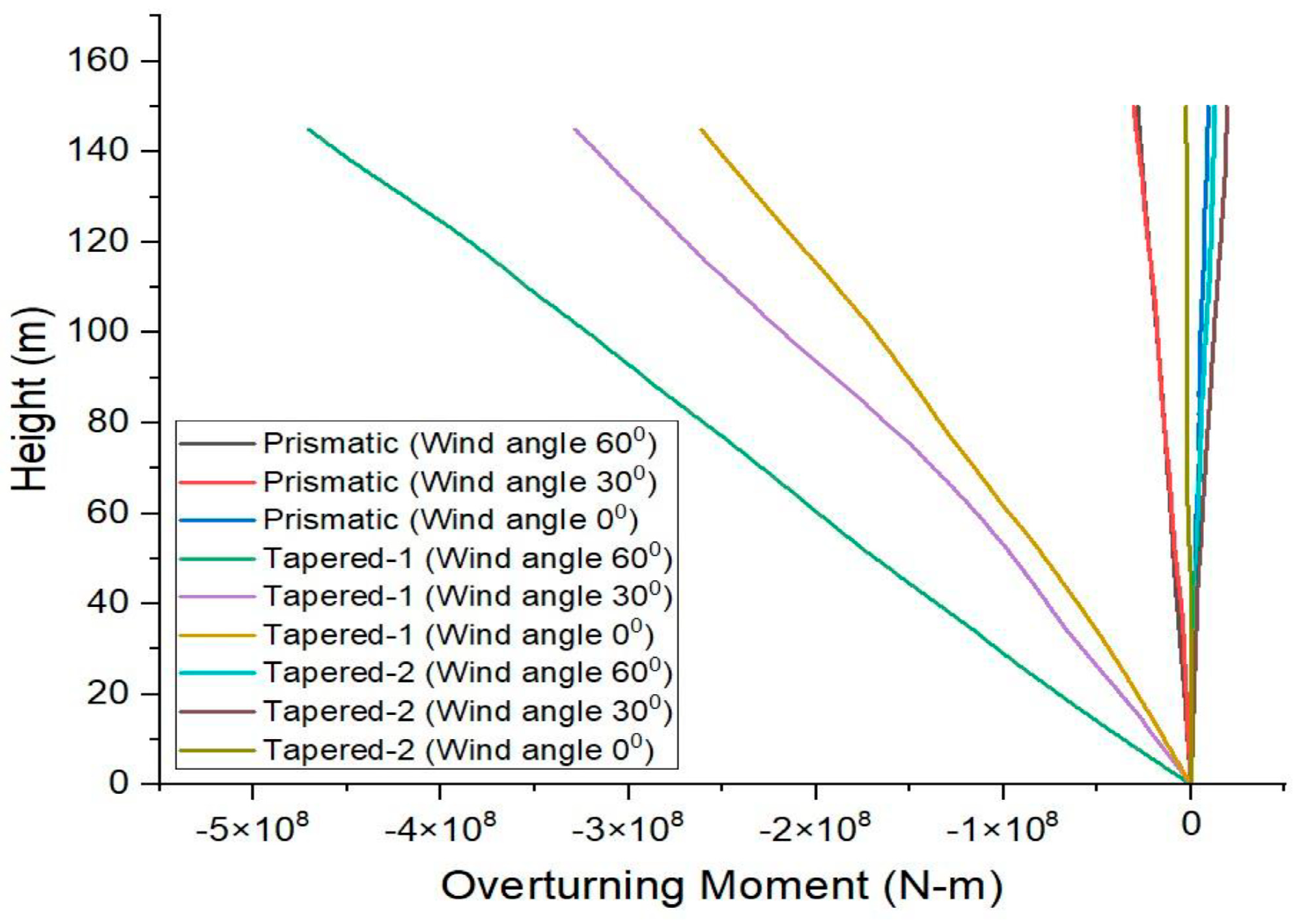
5.2. Variation in Forces and Moments

The calculation for the total wind-induced dynamic forces and base overturning moments involved integrating the surface pressure and tangential stresses across all faces of the building model. A turbulent inflow simulation was used to obtain the across-wind force coefficient (Cl) and along-wind force coefficient (Cd) with flow time, as shown in Figure 15. It is noteworthy that the curves display fluctuating components caused by large wind-induced vortices surrounding the building model, and local vibrations that corresponded to aerodynamic loads from small eddies [57,58].

The aim of the study was to evaluate the impact of wind forces, specifically along-wind and across-wind forces, at different heights of the building model. The study analyzed all models under 0°, 30°, and 60° wind incidence angles. The results showed that the along-wind forces were more dominant under a 60° wind incidence angle compared to the other two angles for each building model. When the model with the tapered-1 shape was analyzed under a 30° wind incidence angle, the across-wind force was more dominant compared to other cases. Suction was highly dominant at 2/3 the height of the building near rounded corners for the tapered-2 building model. It was observed that the across-wind force was minimal for all three models under a 0° wind incidence angle compared to the other two wind incidence angles. Figure 16a,b illustrate the results of the wind forces for the prismatic and tapered-1, 2 shapes. The findings provide valuable insights for designing structures that can efficiently withstand wind forces [14,49].

The data presented in Figure 15c and Figure 17 display the changes in the overturning moment with both time and height for three different building models subjected to various wind incidence angles. The results indicate that a building model with a tapered (40% area reduction) shape experiences higher overturning moments under a 60° wind incidence angle, which then decreases over time, compared to a building with a prismatic shape. Furthermore, the variation in the overturning moment with model height suggests that the tapered-1 shape had higher values with increasing height compared to the two other models. Conversely, compared to the prismatic shape, the tapered shape experienced higher overturning moments [59].

5.3. Displacement and Stresses

The total displacement and equivalent stress contour with mesh movement from the current Fluid-Structure Interaction (FSI) simulation is displayed in Figure 18. The displacement measurements of all three building models were carefully monitored. Figure 19 presents the time histories of the maximum and average deformations of the building model under various wind incidence angles. The CFD mesh nodes on the building surfaces were moved and deformed by the nodes of elements on the vertical center line of the building body, indicating an accurate exchange of loads and response information in the current FSI method. The monitored displacements at the building exhibited distinct patterns in the structural response. The along-wind structural response initially exhibited large amplitudes, gradually damping to smaller ones, possibly due to the combined action of aerodynamic and structural damping. On the other hand, the across-wind structural response showed a continuous increase in amplitude until 5 s, likely due to the synchronization of structural and vortex shedding frequencies.

Figure 18 and Figure 19 depict the total displacement and equivalent stress contours, revealing significant patterns in the structural response. Notably, the initial large amplitudes in the along-wind structural response can be attributed to the onset of resonance effects, which gradually stabilized as the simulation progressed. Conversely, the continuous increase in amplitude in the across-wind structural response until 5 s indicates a persistent aerodynamic excitation, possibly due to vortex shedding. These observations underscore the need for careful consideration of dynamic wind loads in the design of high-rise structures, particularly those with tapered geometries.

6. Conclusions

This paper described the effect of wind-induced vibrations on and aerodynamic responses of a triangular full-scale high-rise building model under turbulent flow conditions. The approach combined structural modal analysis with Computational Fluid Dynamics (CFD) methodologies. The turbulence generation method utilized in this study effectively replicated unsteady wind conditions in the atmospheric boundary layer. Through artificial turbulence, the natural key features of wind were accurately reproduced, and significant vortex shedding around the building model were captured. To determine the dynamic response of the building, a conservative quadrature-projection scheme was employed, transferring the surface wind pressure and tangential stresses to the node elements. The resulting modal analysis allowed for a comprehensive understanding of the building’s behavior. In summary, the significant outcomes of the current study were follows:

• The use of unsteady Computational Fluid Dynamics (CFD) techniques combined with modal analysis constitutes a pragmatic approach for evaluating wind-induced vibrations in tall buildings during the initial design phase. Flow solutions were computed once and then subsequently iteratively employed in the structural dynamics analysis. This investigation completed the structural dynamic analysis, comprising 26,000 iterations, in approximately 72 h.
• The study demonstrated that the wind angle significantly influences the aerodynamic forces acting on the building models. At a 60° wind angle, the maximum drag coefficient was observed to be 3.2 × 10³, while at 30°, the drag coefficient decreased to 2.1 × 10³. This reduction in drag coefficient at higher wind angles indicates the effectiveness of building orientation in reducing wind-induced loads, which is crucial for optimizing the structural design of high-rise buildings.
• The impact of aerodynamic damping on wind-induced vibrations in slender buildings cannot be overstated, especially when motion is considerable. The findings of this study indicate that the aerodynamic damping experienced a significant peak in the across-wind direction, while increasing linearly in the along-wind direction. However, it had minimal effects on mean along-wind responses and determining aerodynamic damping presents a challenge, particularly for structurally complex buildings with irregular appearances.
• The conclusions drawn in this study suggest that a thorough analysis of slender buildings featuring non-regular cross-sections, like triangular shapes, is advisable. Such an analysis should encompass the dynamic effects of wind loads to accurately determine the structure’s behavior. This recommendation aims to enhance the assurance of achieving a well-balanced compromise between safety and economic considerations in the design and construction of such buildings.

References

1. Mattias, L.W.A.; Abdalla Filho, J.E. Dynamic behavior of H-shape tall building subjected to wind loading computed by stochastic and CFD methodologies. Wind Struct. Int. J. 2023, 37, 229–243. [Google Scholar] [CrossRef]
2. Honerkamp, R.; Li, Z.; Isaac, K.M.; Yan, G. Influence of turbulence modeling on CFD simulation results of tornado-structure interaction. Wind Struct. Int. J. 2022, 35, 131–146. [Google Scholar] [CrossRef]
3. Shirzadeh Germi, M.; Eimani Kalehsar, H. Numerical investigation of interference effects on the critical wind velocity of tall buildings. Structures 2021, 30, 239–252. [Google Scholar] [CrossRef]
4. ALMahdi, F.; Fahjan, Y.; Doğangün, A. Critical remarks on Rayleigh damping model considering the explicit scheme for the dynamic response analysis of high rise buildings. Adv. Struct. Eng. 2021, 24, 1955–1971. [Google Scholar] [CrossRef]
5. Chauhan, B.S.; Chakrabarti, A.; Ahuja, A.K. Study of wind loads on rectangular plan tall building under interference condition. Structures 2022, 43, 105–130. [Google Scholar] [CrossRef]
6. Yu, X.F.; Xie, Z.N.; Wang, X.; Cai, B. Interference effects between two high-rise buildings on wind-induced torsion. J. Wind Eng. Ind. Aerodyn. 2016, 159, 123–133. [Google Scholar] [CrossRef]
7. Li, Y.; Zhu, Y.; Chen, F.B.; Li, Q.S. Aerodynamic loads of tapered tall buildings: Insights from wind tunnel test and CFD. Structures 2023, 56, 104975. [Google Scholar] [CrossRef]
8. Yu, X.F.; Xie, Z.N.; Zhu, J.B.; Gu, M. Interference effects on wind pressure distribution between two high-rise buildings. J. Wind Eng. Ind. Aerodyn. 2015, 142, 188–197. [Google Scholar] [CrossRef]
9. Cheng, W.C.; Liu, C.H.; Ho, Y.K.; Mo, Z.; Wu, Z.; Li, W.; Chan, L.Y.L.; Kwan, W.K.; Yau, H.T. Turbulent flows over real heterogeneous urban surfaces: Wind tunnel experiments and Reynolds-averaged Navier-Stokes simulations. Build. Simul. 2021, 14, 1345–1358. [Google Scholar] [CrossRef]
10. Li, G.; Wu, Y.; Yan, C.; Fang, X.; Li, T.; Gao, J.; Xu, C.; Wang, Z. An improved transfer learning strategy for short-term cross-building energy prediction using data incremental. Build. Simul. 2023, 17, 165–183. [Google Scholar] [CrossRef]
11. Dogan, T.; Kastner, P. Streamlined CFD simulation framework to generate wind-pressure coefficients on building facades for airflow network simulations. Build. Simul. 2021, 14, 1189–1200. [Google Scholar] [CrossRef]
12. Kim, Y.C.; Cao, S. Application of probabilistic method to determination of aerodynamic force coefficients on tall buildings. Wind Struct. Int. J. 2023, 36, 249–261. [Google Scholar] [CrossRef]
13. Verma, H.; Sonparote, R.S. Numerical investigation of wind interference effect on twin C-shaped tall buildings. Wind Struct. Int. J. 2023, 37, 425–444. [Google Scholar] [CrossRef]
14. Gu, M.; Su, L.; Quan, Y.; Huang, J.; Fu, G. Experimental study on wind-induced vibration and aerodynamic mitigation measures of a building over 800 meters. J. Build. Eng. 2022, 46, 103681. [Google Scholar] [CrossRef]
15. Paul, R.; Dalui, S.K. Aerodynamic shape optimization of a high-rise rectangular building with wings. Wind Struct. Int. J. 2022, 34, 259–274. [Google Scholar] [CrossRef]
16. Rafizadeh, H.; Alaghmandan, M.; Tabasi, S.F.; Banihashemi, S. Aerodynamic behavior of supertall buildings with three-fold rotational symmetric plan shapes: A case study. Wind Struct. Int. J. 2022, 34, 407–419. [Google Scholar] [CrossRef]
17. Mandal, S.; Dalui, S.K.; Bhattacharjya, S. Wind induced response of corner modified ‘U’ plan shaped tall building. Wind Struct. Int. J. 2021, 32, 521–537. [Google Scholar] [CrossRef]
18. Assainar, N.; Dalui, S.K. Aerodynamic analysis of pentagon-shaped tall buildings. Asian J. Civ. Eng. 2021, 22, 33–48. [Google Scholar] [CrossRef]
19. Ntinas, G.K.; Shen, X.; Wang, Y.; Zhang, G. Evaluation of CFD turbulence models for simulating external airflow around varied building roof with wind tunnel experiment. Build Simul. 2018, 11, 115–123. [Google Scholar] [CrossRef]
20. Zhang, Y.; Habashi, W.G.; Khurram, R.A. Predicting wind-induced vibrations of high-rise buildings using unsteady CFD and modal analysis. J. Wind Eng. Ind. Aerodyn. 2015, 136, 165–179. [Google Scholar] [CrossRef]
21. Tanaka, H.; Tamura, Y.; Ohtake, K.; Nakai, M.; Chul Kim, Y. Experimental investigation of aerodynamic forces and wind pressures acting on tall buildings with various unconventional configurations. J. Wind Eng. Ind. Aerodyn. 2012, 107–108, 179–191. [Google Scholar] [CrossRef]
22. Zhou, L.; Tse, K.T.; Hu, G.; Li, Y. Higher order dynamic mode decomposition of wind pressures on square buildings. J. Wind Eng. Ind. Aerodyn. 2021, 211, 104545. [Google Scholar] [CrossRef]
23. Li, Y.; Li, Q.S.; Chen, F. Wind tunnel study of wind-induced torques on L-shaped tall buildings. J. Wind Eng. Ind. Aerodyn. 2017, 167, 41–50. [Google Scholar] [CrossRef]
24. Sanyal, P.; Dalui, S.K. Effect of corner modifications on Y’ plan shaped tall building under wind load. Wind Struct. Int. J. 2020, 30, 245–260. [Google Scholar] [CrossRef]
25. Paul, R.; Dalui, S.K. Wind-induced Peak Dynamic Responses of ‘Z’ Shaped Tall Building. J. Inst. Eng. Ser. A 2022, 103, 891–904. [Google Scholar] [CrossRef]
26. Bhattacharyya, B.; Dalui, S.K. Investigation of mean wind pressures on ‘E’ plan shaped tall building. Wind Struct. Int. J. 2018, 26, 99–114. [Google Scholar] [CrossRef]
27. Tong, Z.; Chen, Y.; Malkawi, A. Defining the Influence Region in neighborhood-scale CFD simulations for natural ventilation design. Appl. Energy 2016, 182, 625–633. [Google Scholar] [CrossRef]
28. Bairagi, A.K.; Dalui, S.K. Optimization of interference effects on high-rise buildings for different wind angle using CFD simulation. Electron. J. Struct. Eng. 2014, 14, 39–49. [Google Scholar] [CrossRef]
29. Cui, D.J.; Mak, C.M.; Kwok, K.C.S.; Ai, Z.T. CFD simulation of the effect of an upstream building on the inter-unit dispersion in a multi-story building in two wind directions. J. Wind Eng. Ind. Aerodyn. 2016, 150, 31–41. [Google Scholar] [CrossRef]
30. Spalart, P.R.; Allmaras, S.R. RechAerosp_1994_SpalartAllmaras-2. La Rech. A one-equation turbulence model for aerodynamic flows. In Proceedings of the 30th Aerospace Sciences Meeting and Exhibit, Reno, NV, USA, 6–9 January 1992; pp. 5–21. [Google Scholar] [CrossRef]
31. Spalart, P.R.; Jou, W.H.; Strelets, M.K.; Allmaras, S.R. Comments on the feasibility of LES for wings and on a hybrid RANS/LES approach. In Proceedings of First AFOSR International Conference on DNS/LES; Office of Scientific Research, Conference Paper 4–8; Greyden Press: Columbus, OH, USA, 1997. [Google Scholar]
32. Sanyal, P.; Dalui, S.K. Effects of side ratio for ‘Y’ plan shaped tall building under wind load. Build. Simul. 2021, 14, 1221–1236. [Google Scholar] [CrossRef]
33. Hassan, S.; Molla, M.M.; Nag, P.; Akhter, N.; Khan, A. Unsteady RANS simulation of wind flow around a building shape obstacle. Build. Simul. 2022, 15, 291–312. [Google Scholar] [CrossRef]
34. Hadane, A.; Redford, J.A.; Gueguin, M.; Hafid, F.; Ghidaglia, J.M. CFD wind tunnel investigation for wind loading on angle members in lattice tower structures. J. Wind Eng. Ind. Aerodyn. 2023, 236, 105397. [Google Scholar] [CrossRef]
35. Bre, F.; Gimenez, J.M. A cloud-based platform to predict wind pressure coefficients on buildings. Build. Simul. 2022, 15, 1507–1525. [Google Scholar] [CrossRef]
36. Cheung, J.O.P.; Liu, C.H. CFD simulations of natural ventilation behaviour in high-rise buildings in regular and staggered arrangements at various spacings. Energy Build. 2011, 43, 1149–1158. [Google Scholar] [CrossRef]
37. Bairagi, A.K.; Dalui, S.K. Wind environment around the setback building models. Build. Simul. 2021, 14, 1525–1541. [Google Scholar] [CrossRef]
38. Shirzadi, M.; Mirzaei, P.A.; Tominaga, Y. CFD analysis of cross-ventilation flow in a group of generic buildings: Comparison between steady RANS, LES and wind tunnel experiments. Build. Simul. 2020, 13, 1353–1372. [Google Scholar] [CrossRef]
39. Toja-Silva, F.; Kono, T.; Peralta, C.; Lopez-Garcia, O.; Chen, J. A review of computational fluid dynamics (CFD) simulations of the wind flow around buildings for urban wind energy exploitation. J. Wind Eng. Ind. Aerodyn. 2018, 180, 66–87. [Google Scholar] [CrossRef]
40. Kato, S.; Murakami, S.; Takahashi, T.; Gyobu, T. Chained analysis of wind tunnel test and CFD on cross ventilation of large-scale market building. J. Wind Eng. Ind. Aerodyn. 1997, 67–68, 573–587. [Google Scholar] [CrossRef]
41. Thordal, M.S.; Bennetsen, J.C.; Koss, H.H.H. Review for practical application of CFD for the determination of wind load on high-rise buildings. J Wind Eng. Ind. Aerodyn. 2019, 186, 155–168. [Google Scholar] [CrossRef]
42. Yadav, H.; Roy, A.K.; Kumar, A.; Kumar, A.; Chauhan, N.; Kumar, V. Analysis of retaining walls along the Beas River’s meandering curve. Structures 2023, 54, 527–540. [Google Scholar] [CrossRef]
43. Blocken, B.; Stathopoulos, T.; Carmeliet, J. CFD simulation of the atmospheric boundary layer: Wall function problems. Atmos. Environ. 2007, 41, 238–252. [Google Scholar] [CrossRef]
44. Ramponi, R.; Blocken, B. CFD simulation of cross-ventilation for a generic isolated building: Impact of computational parameters. Build. Environ. 2012, 53, 34–48. [Google Scholar] [CrossRef]
45. Feng, C.; Gu, M.; Zheng, D. Numerical simulation of wind effects on super high-rise buildings considering wind veering with height based on CFD. J. Fluids Struct. 2019, 91, 102715. [Google Scholar] [CrossRef]
46. Yadav, H.; Roy, A.K.; Kumar, A. The influence of interactions between two high-rise buildings on the wind-induced moment. Asian J. Civ. Eng. 2023, 25. [Google Scholar] [CrossRef]
47. AIJ. AIJ Recommendations for Loads on Buildings; Architectural Institute of Japan: Tokyo, Japan, 2019. [Google Scholar]
48. Yi, Y.K.; Feng, N. Dynamic integration between building energy simulation (BES) and computational fluid dynamics (CFD) simulation for building exterior surface. Build. Simul. 2013, 6, 297–308. [Google Scholar] [CrossRef]
49. Rizzo, F.; Ricciardelli, F.; Maddaloni, G.; Bonati, A.; Occhiuzzi, A. Experimental error analysis of dynamic properties for a reduced-scale high-rise building model and implications on full-scale behaviour. J. Build. Eng. 2020, 28, 101067. [Google Scholar] [CrossRef]
50. Rizzo, F.; Ierimonti, L.; Venanzi, I.; Sacconi, S. Wind-induced vibration mitigation of video screen rooms in high-rise buildings. Structures 2021, 33, 2388–2401. [Google Scholar] [CrossRef]
51. NBR 6123; Associação Brasileira De Normas Técnicas. ABNT: Rio de Janeiro and São Paulo, Brazil, 1988; Volume 69, ISBN 978-85-07-09955.
52. IS-16700; Criteria for Structural Safety of Tall Concrete Buildings. Bureau of Indian Standards (BIS): New Delhi, India, 2023.
53. Eurocode-1. Eurocode-1. Eurocode 1—Actions on structures. Actions Struct—Part 1-4. In Dictionary Geotechnical Engineering/Wörterbuch GeoTechnik; Springer: Berlin/Heidelberg, Germany, 2014; Volume 86, pp. 315–326. [Google Scholar] [CrossRef]
54. ASCE/SEI 7-10; Minimum Design Loads and Associated Criteria for Buildings and Other Structures. Structural Engineering Institute of the American Society of Civil Engineering: Reston, VA, USA, 2013.
55. Ha, T.; Shin, S.H.; Kim, H. Damping and natural period evaluation of tall RC buildings using full-scale data in Korea. Appl. Sci. 2020, 10, 1568. [Google Scholar] [CrossRef]
56. Rizzo, F. Investigation of the time dependence of wind-induced aeroelastic response on a scale model of a high-rise building. Appl. Sci. 2021, 11, 3315. [Google Scholar] [CrossRef]
57. Rizzo, F.; D’Alessandro, V.; Montelpare, S.; Giammichele, L. Computational study of a bluff body aerodynamics: Impact of the laminar-to-turbulent transition modelling. Int. J. Mech. Sci. 2020, 178, 105620. [Google Scholar] [CrossRef]
58. Rizzo, F.; Huang, M. Peak value estimation for wind-induced lateral accelerations in a high-rise building. Struct. Infrastruct. Eng. 2022, 18, 1317–1333. [Google Scholar] [CrossRef]
59. Rizzo, F.; Caracoglia, L.; Piccardo, G. Examining wind-induced floor accelerations in an unconventionally shaped, high-rise building for the design of “smart” screen walls. J. Build. Eng. 2021, 43, 103115. [Google Scholar] [CrossRef]
Figure 1. (a) Computational domain and (b) arrangements and cross-section details of models used for numerical study.
Buildings 14 02722 g001
Figure 2. Flow chart of simulation study.
Buildings 14 02722 g002
Figure 3. Mesh pattern around the building.
Buildings 14 02722 g003
Figure 4. Pressure coefficient values for validation from wind tunnel test [5] and CFD simulation (Spalart–Allmaras DES model).
Buildings 14 02722 g004
Figure 5. Velocity contour of computational domain.
Buildings 14 02722 g005
Figure 6. Turbulence intensity profile.
Buildings 14 02722 g006
Figure 7. Mean velocity profile.
Buildings 14 02722 g007
Figure 8. The vibration mode shape and natural frequencies of the building model.
Buildings 14 02722 g008
Figure 9. Mean pressure coefficient for a triangular building.
Buildings 14 02722 g009
Figure 10. Velocity streamlines at a building height of 125 m from base level.
Buildings 14 02722 g010
Figure 11. Velocity streamlines at y = 0 m from base level.
Buildings 14 02722 g011
Figure 12. (a) Flow pattern and (b) Karman vortex shedding on leeward side of the prismatic building.
Buildings 14 02722 g012
Figure 13. Iso-surface (Q-criterion value: 0.02) of turbulence structure around the building under 0° wind incidence angle.
Buildings 14 02722 g013
Figure 14. (a) Average across-wind vortex velocity with flow time. (b) Power spectral density of Uy.
Buildings 14 02722 g014
Figure 15. Variation in (a) Cd, (b) Cl, and (c) overturning moment with flow time.
Buildings 14 02722 g015
Figure 16. Variation in (a) along-wind forces and (b) across-wind forces with height of building model.
Buildings 14 02722 g016
Figure 17. Variation in overturning moment with height of building model.
Buildings 14 02722 g017
Figure 18. Total deformation of principal building.
Buildings 14 02722 g018
Figure 19. (a) Max deformation and (b) average deformation of building model under 0°, 30°, and 60° wind incidence angles.
Buildings 14 02722 g019